Selçuk J. Appl. Math. Selçuk Journal of Vol. 8. No.1. pp. 57-74 , 2007 Applied Mathematics
A Comparative Study of Fixed Effects Models and Random Inter-cept/Slope Models as a Special Case of Linear Mixed Models for Repeated Measurements
Neslihan ˙Iyit and A¸sır Genç
Selcuk University, Faculty of Arts and Sciences, Department of Statistics, Campus, 42010, Konya, Turkey
e-mail:niyit@ selcuk.edu.tr,agenc@ selcuk.edu.tr
Received : December 29, 2006
Summary. Any dataset in which subjects are measured repeatedly over time or space can be described as repeated measurements data. A linear mixed model (LMM) is a powerful method for analyzing repeated measurements data. It is made up of two components. The first component consists of a regression model for the average response over time and the effects of covariates on this average response. The second component provides a model for the pattern of covariances or correlations between the repeated measurements. In this study, a comparative evaluation of fixed effects models with random intercept models and random intercept and slope models as a special case of random effects models from linear mixed models are taken into consideration and the superiority of random intercept and slope models allow to modeling possible heterogeneity in intercepts and in slopes of the individual’s own regression line for repeated measurements data is emphasized
Key words: Repeated measurement, linear mixed model, fixed effects model, random effects model, random intercept model, random intercept and slope model, compound symmetry pattern, Mauchly’s sphericity test.
1. Introduction
The defining feature of a longitudinal study design is that measurements of the same individuals are taken repeatedly through time allowing the direct study of change over time. The primary goal of a longitudinal study is to characterize the change in response over time and the factors that influence change (Fitzmau-rice et al., 2004). Analyzing such a repeated measurements data on individuals requires recognizing and estimating variability both between and within indi-viduals. The linear mixed model approach to repeated measurements allows
explicit modeling and analysis of this variation between-subjects and within-subjects factors (Davis, 2002). A factor consisting of repeated measurements on the same subjects or experimental units, under different conditions is commonly called a “within-subjects” factor. A “between-subjects” factor is one in which each level of the factor contains different experimental units (˙Iyit et al., 2006). Linear mixed models (LMMs) provide a tool for analyzing repeated measure-ments data by taking into consideration these two types of variability as well as the linear relationship between the explanatory variables and the response variable (McCulloch and Searle, 2001).
The theoretical base of linear mixed models is well-established and the method-ology has applications in many areas not only involving repeated measurements. McLean et al. (1991) provide a general introduction to linear mixed models and Ware (1985) gives an overview of their application to the analysis of repeated measurements. Raudenbush and Bryk (2002) investigate random intercept mod-els and random intercept and slope modmod-els in details and Bryk and Driscoll (1988) use these two model types to examine how characteristics of school or-ganization are related to teachers’ sense of efficacy in their work in the field of education.
In this study a comparative evaluation of fixed effects models with random intercept models and random intercept and slope models as a special case of random effects models from linear mixed models are taken into consideration and the superiority of random intercept and slope models allows to modeling possible heterogeneity in intercepts and in slopes of the individual’s own regression line for repeated measurements data is emphasized.
This paper is organized as follows; In Section 2 a general introduction to linear mixed models is given and then fixed effects models and random intercept/slope models as a special case of random effects models from linear mixed models are introduced also the information criteria in model selection of fixed and random effects models are given. In Section 3 an application of a statistical analysis of repeated measurements data with both fixed effects models and random effects models is considered. Results and discussion also conclusion parts obtained from the analysis with these procedures are given in Section 4 and Section 5 respectively.
2. Linear Mixed Models for Repeated Measurements
A model where we have both fixed effects and random effects is called mixed model because of the mixture of different types of these effects on response variable. Fixed effects are the effects attributable to a finite set of levels of a factor on response variable representing all possible levels of the variable in which inferences are to be made. On the other hand random effects are the ones attributable to an infinite set of levels of a factor on response variable of which only a random sample of potential levels of the factor is taken to draw inferences for the complete population of levels (Searle et all., 1992). In mixed models fixed effects are used to explain the expected value of the observations and random effects to explain the variance-covariance structure of the dependent variable
(Hamer and Simpson, 1989). If the relationship between the observations of the response variable and these effects is linear, then the model is called linear mixed model (Davis, 2002).
Laird and Ware (1982) consider the LMM in matrix notation;
(1) = X + Z +
where ×1is the vector of response variables, X×is the known design matrix
for fixed effects parameter vector,
×1 is the unknown fixed effects parameter
vector, Z× is the known design matrix for random effects vector, ×1 is the
unobserved random effects vector for =
P
=1
having ()×1 sub-vectors for
= 1 2 random effects included in the model such as;
(2) =£ 1 2 · · · ¤0
and corresponding (Z)×sub-matrices for = 1 2 random effects given
by Eq.(2) included in the model such as;
(3) Z=£ Z1 Z2 · · · Z
¤
and ×1is the unobserved vector of the independent and identically distributed Gaussian random error terms (McLean et al.,1991). The mean vector and the variance-covariance matrix for the components of LMM are as follows;
(4) () = 0 () = (0) = D ⇒ ∼ (0 D) (5) () = 0 () = (0) = R = 2I ⇒ ∼ (0 R ) (6) ( 0) = ( 0) = 0 Then (7) ( ) = X ( ) = V = ZDZ0+ R ⇒ ∼ ¡X ZDZ0+R¢ In repeated measurements designs ZDZ0represents the between-subject portion of the covariance structure and R represents the within-subject portion of the covariance structure.
Parameters in LMMs are estimated by maximum likelihood (ML) or by a tech-nique known as restricted maximum likelihood (REML). For ×1; the vector of
response variables having the assumption given by Eq.(7), the likelihood func-tion of the parameters and V having elements known as variance components 2; = 0 1 2 ¡20= 2 ¢ is as follows; (8) ln ¡V¢= − 2 ln (2) − 1 2ln |V| − 1 2 ¡ − X¢0V−1¡ − X¢ The ML equations that maximize the likelihood function given by Eq.(8) for a P×; symmetric square matrix satisfying
(9) P= V−1− V−1X¡X0V−1X¢−X0V−1= K (K0VK)−1K0 condition are as follows;
(10) ³X0Vˆ−1X´ˆ = X ˆV−1
(11) ³Vˆ−1ZZ0
´
= 0PZˆ Z0Pˆ = 0 1 2
where 0 = 20 = 2 0 = Z0 = I. On the other hand the
second ML equation given by Eq.(11) is nonlinear with respect to the variance components occurred in V−1. Thus closed form expressions for the solutions
of Eq.(11) can be obtained iteratively by Newton-Raphson or Fisher’s Scoring algorithms (Searle et al., 1992).
For ×1; the vector of response variables having the assumption given by Eq.(7), REML method is based on K0 ; linear combinations of elements of the
responses chosen in such a way that those combinations do not contain any fixed effects satisfying K0X = 0 condition for a K0 = £0
1 02 0−
¤
matrix having elements − linearly independent 0 vectors satisfying 0X= 0 by
making suitable replacements,
(12) K0
X K0X= 0 and
Z K0Z V K0VK
Then the restricted likelihood function of the parameter K0VK having only
variance components for
(13) K0 ∼ ¡0 K0VK¢ is as follows; (14) ln (K0VKK0 ) = −( − ) 2 ln (2)− 1 2ln |K 0VK|−1 2 0K(K0VK)−1K0
Then the REML equations that maximize the restricted likelihood function given by Eq.(14) for a P×matrix satisfying Eq.(9) are as follows;
(15) ³PZb Z0
´
= 0PZb Z0Pb = 0 1 2
Again the REML equations given by Eq.(15) are nonlinear with respect to the variance components occurred in P matrix including V−1 can be obtained it-eratively by Newton-Raphson or Fisher’s Scoring algorithms (McCulloch and Searle, 2001).
From Eq.(1) it can be easily seen that fixed effects model is a special case of LMM when Z = 0 and R = σ2I¯.. Random effects models are special case of
linear mixed models. The main importance of random effects models for longitu-dinal data is the necessity of modeling natural heterogeneity across individuals in their response profile over time. In the following subsections fixed effects models, random intercept model and random intercept and slope model from random effects models as a special case of linear mixed models are taken into consideration.
2.1. Fixed Effects Models
A fixed effects model or commonly called general linear model (GLM) for the statistical analysis of such a repeated measurements design includes only mod-eling the expected value of the observations as a linear function of explanatory variables based on the assumption that the observations from different subjects are statistically independent and uncorrelated and that the variance-covariance structure is the same for each subject (Landau and Everitt, 2004). The fixed effects model for the response given by individual at time is modeled as;
(16) = 0+ 1() + 2+
where is the dummy variable indicating the treatment group to which
individual belongs, 0 1 and 2 are the usual regression coefficients for the model; 0 is the intercept, 1 represents the treatment group effect and 2the slope of the linear regression of outcome on time. is the usual residual or
error term, assumed to be normally distributed with zero mean and variance 2.
Fixed effects model analysis in repeated measurements data is valid under three assumptions about the data:
1.Normality : the data arise from populations with normal distribution. 2.Homogeneity of variance: the variances of the assumed normal distribu-tions are equal. Levene (1960) developed a test statistic for testing the homo-geneity of variance assumption using the F distribution with − 1 and − degrees of freedom at a significance level of that is −1 − called Levene
(17) = ( − ) P =1 ¡− ¢ 2 ( − 1) P =1 P =1 ¡ − ¢ 2
where is the total number of subjects, is the number of groups, is the
number of subjects in the group,
are the group means of the ,
is the overall mean of the and is defined as = |− | and as
=
P
=1
the mean of the group.
3.Sphericity condition: the covariance matrix of the observations must have compound symmetry pattern given by Eq.(22). Mauchly (1940) developed a test statistic for testing the sphericity assumption using the chi-square distribution called Mauchly’s sphericity test. The formulas for Mauchly’s test statistic are as follows; (18) =¯¯CSC0¯¯ ¡CSC0¢ (19) 2(+1)2−1= − ÃX =1 − ! ⎛ ⎜ ⎜ ⎜ ⎜ ⎝1 − 22+ + 2 6 ÃX =1 − ! ⎞ ⎟ ⎟ ⎟ ⎟ ⎠ln ( )
where is the number of parameters in the model, is the number of groups, is the number of subjects in the group, C is a contrast matrix with
rows suitable for testing a main effect or interaction, S is a × matrix of the pooled group covariances;
(20) S= P =1 P =1 (− ) (− )0 P =1 − where = P =1
is the mean of the group (Rencher, 1995).
When the last assumption is not thought to be valid, then LMMs having flexible covariance structures are used to analyze data in repeated measurements design (Landau and Everitt, 2004).
On the other hand making such a restrictive assumption like repeated measure-ments of a response variable are independent and uncorrelated with the same
variance-covariance structure for each subject is an unrealistic assumption for modeling longitudinal data. Because of this reason random effects models al-lowing within-group correlations between repeated measurements and modeling the covariance structure of each subject given in the following subsection are better than fixed effects models (Wolfinger and Chang, 1999).
2.2. Random Effects Models
Suppose that we have observations made in a repeated measurements study at time points 1 2 . Assume that we have a single covariate called
treatment group coded as a zero or one dummy variable. We want to model the response of an individual at time point in terms of treatment group and
time. We assume that there is no treatment ×time interaction. For this aim two possible random effects model types called random intercept model and random intercept and slope model can be used to model individuals’ responses over time 2.2.1. Random Intercept Model
The simplest case of a linear mixed model is the random intercept model based on the fixed effects model with a randomly varying subject effect. The random intercept model for the response given by individual at time is modeled
as;
(21) = 0+ 1() + 2+ +
where group is the dummy variable indicating the treatment group to which
individual belongs, 0 1 and 2 are the usual regression coefficients for the model; 0 is the intercept, 1 represents the treatment group effect and
2 the slope of the linear regression of response variable on time. is the
usual residual or random error term, assumed to be normally distributed with mean zero and variance 2 that is
∼ (0 2). terms are the random
effects that model possible heterogeneity in the intercepts of the individuals and are assumed normally distributed with zero mean and variance 2
that is ∼ ¡ 0 2 ¢
. The and terms are assumed independent of one another
that is ( ) = 0.
In the random intercept model each individual’s trend over time is assumed parallel to the treatment group’s average trend only the intercepts of each in-dividual’s regression line differ by including the random subject effect term
Figure1. Graphical illustration of random intercept model by time versus response
The presence of the terms specifies modeling covariance pattern for the
re-peated measurements of the response variable by an appropriate covariance matrix called compound symmetry (CS) pattern as follows;
(22) = ⎡ ⎢ ⎢ ⎣ σ2 + σ2 σ2 σ2 σ2 σ2 σ2+ σ2 σ2 σ2 σ2 σ2 σ2+ σ2 σ2 σ2 σ2 σ2 σ2+ σ2 ⎤ ⎥ ⎥ ⎦
where 2 represents variance within subjects that is (
) = 2, and 2;
covariance between measurements within subjects or variance between subjects for repeated measurements on the subject that is (
) = 2 (˙Iyit et al.,
2006). As seen from Eq.(22) compound symmetry (CS) covariance structure defines equal variances and covariances between measurements with the same diagonal elements given by 2 + 2 and the off-diagonal elements given by
2
. So this structure is very important to satisfy the sphericity assumption as
mentioned in Section 2.1.
On the other hand this covariance structure satisfying sphericity assumption is not realistic for most repeated measurements data because it specifies that each pair of the repeated measurements on the same subject is equally correlated. It seems reasonable that the observations closer in time will be more highly correlated then those taken further apart from the same subject.
2.2.2. Random Intercept and Slope Model
A model that allows a more realistic structure than the random intercept model for specifying covariance structures of the observations is called random intercept
and slope model that allows heterogeneity in both intercepts and slopes (˙Iyit and Genç, 2005a,b).The random intercept and slope model for the response given by individual at time is modeled as;
(23) = 0+ 1() + 2+ 1+ 2+
where 1and 2terms are the random effects that model possible heterogeneity
in intercepts and in slopes of the individual’s own regression line respectively and are assumed bivariate normally distributed with zero means, variances 2
1,
2
2 and covariance 12.
In the random intercept and slope model each individual’s trend over time is not assumed parallel to the treatment group’s average trend as in random intercept model so the intercepts and slopes of each individual’s regression line differ in this case by including the random subject effect terms 1and 2into the model
is graphically illustrated in Figure 2.
Figure2. Graphical illustration of random intercept and slope model by time versus response
This flexibility ensures the random intercept and slope model to model the co-variance matrix of the repeated measurements with a more complex pattern allowing variances and covariances to change over time. These two advantages make the random intercept and slope model superior in the competition with the random intercept model in random effects models.
2.3. Model Selection in Fixed and Random Effects Models
Likelihood ratio (LR) test obtained by taking twice the difference in the respec-tive maximized log-likelihoods;
(24) 2= 2 (log − log )
compared with a chi-square distribution with degrees of freedom equal to the difference between the number of parameters in the full and reduced models or the information criteria shown below can be used as a goodness-of-fit statistics to test whether one model is significantly better than the other (Landau and Everitt, 2004, Fitzmaurice et all., 2004);
(25) Akaike’s Information Criterion; = −2 log + 2 Hurvich ve Tsai’s Criterion; = −2 log + 2 ( ( − − 1)) Bozdogan’s
Criterion; = −2 log + (log () + 1) Schwarz’s Bayesian
Information Criterion; = 2 log + log ()
where logL is the maximized likelihood (ML) or maximized restricted log-likelihood (REML), is the total number of parameters in the model (ML) or number of parameters in the covariance structure (REML) and is the number of subjects included in the data set. The smaller the information criteria, the better the model happens to be (Fitzmaurice, 2004).
3. Application
The data used in this study are taken from a placebo controlled clinical trial of a treatment for post-natal (PND) depression in psychiatry given by Landau and Everitt (2004). Around 1 in every 10 women has PND after having a baby starting within a month of the birth up to six months later. A mother who suffers from PND shows some symptoms such as feeling depressed, guilty and anxious, getting irritable with her baby, being tired and sleepless, unable to enjoy anything and unable to cope with her baby (Wheatley, 2005). On the other hand the hormones play an important role on women with PND. It is known that levels of estrogen hormone drop suddenly after the baby is born (Lawrie et all., 2004, Gregoire et all., 1996). This trial is designed to assess the effectiveness of an estrogen treatment compared with a placebo treatment for patients suffer from PND. The main outcome measure used in this trial is depression scores recorded on eight monthly visits.
The main interest about these data is to determine whether the estrogen treat-ment helps reduce PND by using the appropriate random effects models. The data handed are for 63 patients, 27 in the placebo treatment group and 36 in the estrogen treatment group. These kind of data are repeated measurements data with time as the single subject factor which explains the within-subject variability, i.e., they are longitudinal data and treatment group as the
between-subject factor which explains the between-subject variability coded as follows: placebo treatment=0, estrogen treatment=1.
In this study fixed effects models and random effects models such as random intercept model, random intercept and slope model as a special case of linear mixed models are fitted to the repeated measurements data by using SPSS 13.0 for Windows package programme.
The variables that we wish to include in the linear mixed model are defined as follows; measure of depression scores recorded on eight monthly visits is spec-ified as dependent variable labeled depscores (at 1 month after start of the treatment: depscores1m up to 8 months after start of the treatment: dep-scores8m). The effect of time factor having levels with values 1 up to 8 months modeled by a linear effect of generating a continuous variable labeled c_month by recoding the time factor levels and standardizing them and treatment effect labeled treat ment as a categorical explanatory variable are taken as fixed ef-fects and a subject identifier (subject ) is included into the model as a random effect.
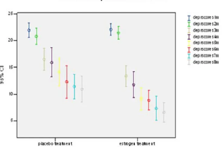
In order to get a first impression of the data a clustered error bar graph corre-sponding to the treatment groups for repeated measurements is given in Figure 3.
Figure 3. Clustered error bargraph for PND repeated measurements data
From Figure 3 it can be concluded that the depression scores are tending to decrease over time in both treatment groups with an apparent larger decrease in the estrogen treatment group at 3 months after starting the treatment. Before fitting either of the fixed and random effects models to the repeated mea-surements data it is important to examine the correlational structure of the de-pression scores within each treatment group correlation matrices. In the placebo treatment group generally there is an apparent first increase and then decrease in the strength of the correlations with increasing length of time between the
repeated measurements and in the estrogen treatment group the strength of the correlations is tending to increase also including irregular patterns with respect to the time. So the statistical analysis of such a repeated measurements de-sign including modeling within-subject variance-covariance structure depends on such a restrictive assumption that the repeated measurements of the out-come variable are independent, uncorrelated with the same variance-covariance structure for each subject is an invalid assumption for modeling the PND scores data. Because of this reason random effects models allowing within-treatment group correlations between repeated measurements and modeling the covariance structure of each subject are better than fixed effects models.
Modeling the PND scores data with the fixed effects model includes an intercept parameter, two regression coefficients for each of the explanatory variables and the variance parameter of the residual terms in the fitted fixed effects model. The “Estimates of Fixed Effects” table given by Table 1 gives the t-tests and associated p-values for assessing the regression coefficients. For a model includ-ing only fixed effects the results suggest that the intercept term and the fixed effects of time (c_month) and treatment explanatory variables are statistically significant at the 5% significance level and are predictive of modeling the PND scores repeated measurements data.
Table 1.Estim atesof Fixed Effects for Fixed Effects M o del
95% Confi dence Interval
Param eter Estim ate Std. Error df t Sig. Lower Bound Upp er Bound Intercept 15.286 0.403 416 37.966 0.000 14.495 16.077 treatm ent -2.641 0.519 416 -5.088 0.000 -3.661 -1.621 c_ m onths -4.806 0.255 416 -18.826 0.000 -5.307 -4.304
The fixed effects model for the PND scores repeated measurements data is a multiple regression model in which there is no random effect as follows;
(26) = 15286 − 2641 () − 4806+
The “Estimates of Covariance Parameters” table given by Table 2 gives details of the single covariance parameter in the fixed effects model, namely, the variance of the residual term. This table provides an estimate, confidence interval and test for zero variance. The variance of the residual term is clearly not zero as seen from the confidence interval for the parameter [23.708, 31.112] given in Table 2 which gives an alternate test, the Wald test (Wald z=14.422, p0.05), for testing the null hypothesis that the variance parameter is zero.
Table 2. Estim ates of Covariance Param eters for Fixed Effects M o del 95% Confidence Interval
Param eter Estim ate Std. Error Wald Z Sig. Lower Bound
Upp er Bound
R esidual 27.159 1.883 14.422 0.000 23.708 31.112
On the other hand the Mauchly’s test statistic for testing the sphericity assump-tion that is the covariance matrix of the observaassump-tions have compound symmetry pattern is rejected with Mauchly’s W-value; 0.062 and related 2-value; 112.562, p-value less than 0.05.
Now we shall fit some random effects models proper to the PND scores data, beginning with the random intercept model. Modeling the PND scores data with the random intercept model indicates that subject random effects for the intercept have been added to the model. This results in fitting one extra model parameter, the variance of the subject random effects.
In the random intercept model case for the PND scores data, it can be easily seen from Table 3 and Table 4 that the model includes an intercept parameter, two regression coefficients; one for each of the explanatory variables and the variance parameters of the residual and the intercept terms in the model.
Table 3. Estim ates of Fixed Effects for Random Intercept M o del
95% Confidence Interval
Param eter Estim ate Std. Error df t Sig. Lower
Bound Upp er Bound Intercept 15.221 0.719 63.076 21.155 0.000 13.784 16.659 treatm ent -2.308 0.945 61.317 -2.443 0.017 -4.197 -0.419 c_ m onths -4.738 0.206 376.242 -23.033 0.000 -5.143 -4.334
The random intercept model allowing to model possible heterogeneity in the intercepts of the individuals for the PND scores repeated measures data is as follows;
(27) = 15221 − 2308 () − 4738+ +
From Table 4, for testing the null hypothesis that the variance of the residual term and the subject intercept effect are zero, the Wald test (Wald z=13.350 and 4.422, p0.05) results and the confidence intervals for the parameters [14.019, 18.804] and [6.997, 16.979] respectively show that the covariance parameters are statistically significantly different from zero.
Table 4. Estim ates of Covariance Param eters for Random Intercept M odel 95% Confidence Interval
Param eter Estim ate Std. Error Wald Z Sig. Lower
Bound
Upp er Bound
Residual 16.237 1.216 13.350 0.000 14.019 18.804
Intercept [sub ject
ID diagonal SC] 10.899 2.465 4.422 0.000 6.997 16.979
Finally modeling the PND scores data with the random intercept and slope model indicates that both the intercept term and the regression coefficient of time effect (c_month) are allowed to vary between subjects. This case results in fitting two extra model parameters to the model, the variance of the subject intercept random effects and the variance of the random slope effects.
From Table 5 the finally fitted random intercept and slope model describes the average profiles of the PND scores data in the two treatment groups over the eight time point visits including random intercepts for subjects and fixed effects of treatment and time.
Table 5. Estim ates of Fixed Effects for Random Intercept and Slop e M o del 95% Confidence Interval
Param eter Estim ate Std. Error df t Sig. Lower
Bound Upp er Bound Intercept 15.307 0.618 110.534 24.783 0.000 14.083 16.531 treatm ent -2.521 0.801 108.131 -3.148 0.002 -4.108 -0.934 c_ m onths -4.773 0.394 108.341 -12.125 0.000 -5.554 -3.993
The random intercept and slope model allowing to model possible heterogeneity in intercepts and in slopes of the individual’s own regression line for the PND repeated measurements data is as follows:
(28) = 15307 − 2521 () − 4773+ 1+ 2+
From Table 6, for testing the null hypothesis that the variance of the residual term and the variance of the subject intercept random effect and the random slope effect are zero, the Wald test (Wald z=12.314 and 5.569, p0.05) results and the confidence intervals for these parameters [12.034, 16.544] and [4.693, 9.487] respectively show that the covariance parameters are statistically signifi-cantly different from zero. Then it can be concluded that the random intercept and slope model provides an adequate description of the PND scores data.
Table 6. Estim ates of Covariance Param eters for R andom Intercept and Slop e M o del 95% Confidence Interval
Param eter Estim ate Std. Error Wald Z Sig. Lower
Bound
Upp er Bound
Residual 14.110 1.146 12.314 0.000 12.034 16.544
Intercept+
c_ m onths [sub ject ID diagonal SC]
6.672 1.198 5.569 0.000 4.693 9.487
The “Information Criteria” table given by Table 7 will be helpful for comparing the fixed effects model and the random intercept model with the finally fitted random intercept and slope model. The information criteria are displayed in Table 7 in smaller-is-better forms.
Tablo 7. Inform ation Criteria for Fixed Effects M odels and Random Intercept/Slop e M o dels Fixed Effects
M o del
Random Intercept M o del
R andom Intercept and Slop e M odel -2 R estricted Log
Likeliho o d 2570.748 2457.092 2370.748
Akaike’s Inform ation
Criterion (AIC) 2572.748 2461.092 2374.748
Hurvich and Tsai’s
Criterion (AICC) 2572.757 2461.121 2374.777
Bozdogan’s
Criterion (CAIC) 2577.778 2471.154 2384.809
Schwarz’s Bayesian
Criterion (BIC) 2576.778 2469.154 2382.809
From Table 7 the difference in -2×restricted log likelihood for the three mod-els can be tested as a chi-square distribution with degrees of freedom given by the difference in the number of parameters in each of the three models. This is known as likelihood ratio test. Here the difference between the fixed effects model likelihood and the random intercept model likelihood is 2570.748-2457.092=113.656, which is tested as a chi-square with one degree of freedom,2
1 095=
384 has an associated p-value 0.01. So the random intercept model is found better than the fixed effects model. When we compare the random intercept model with the random intercept and slope model, the difference between these two model likelihoods is 2457.092-2370.748=86.344 with the same chi-square and associated p-value. Then the random intercept and slope model clearly provides a better fit for the PND scores data than the random intercept model. On the other hand in the light of the other information criteria, the lower the information criteria, the better fit the random intercept and slope model has.
There are a number of residual diagnostics that can be used to check the as-sumptions of a linear mixed model. Firstly the assumption of normality of the random effect terms will be checked by constructing histograms of the variables; residuals and random effects for subjects given by Figure 4.
Figure 4. Histograms for estimates of random effects
The resulting histogram given by Figure 4 does not indicate any departure from the normality assumption. The next one that will be checked is the assumption of homogeneity of variance that is the constant error variance across repeated measurements. For checking this assumption Levene test is used to test the null hypothesis that the error variance of the dependent variable is equal across groups and not rejected with F-value; 0.067 and related p-value; 0.797.
4. Results and Discussion
In this study a comparative evaluation of fixed effects models with random intercept models and random intercept and slope models as a special case of random effects models from linear mixed models are taken into consideration following a repeated measurements design having one between-subject factor (referred to as treatment) with two treatment levels and one within-subject continuous covariate (referred to as time).
Before fitting either of the fixed and random effects models to the repeated measurements data, the correlational structure of the PND scores within each treatment group correlation matrices is examined and it is observed that gen-erally covariances between observations made closer together in time are likely to be higher than those made at greater time points. So the fixed effects model including only modeling the expected value of the observations as a linear func-tion of explanatory variables based on the assumpfunc-tion that the observafunc-tions from different subjects are statistically independent and uncorrelated and that the variance-covariance structure is the same for each subject is not found appro-priate for the statistical analysis of such a repeated measurements design. Also as a result of Mauchly’s test for testing the null hypothesis that the covariance matrix of the observations have compound symmetry pattern is rejected then the sphericity assumption is not satisfied for constructing fixed effects models fitted
to PND scores repeated measurements data. On the other hand the random intercept model implying a particular structure for the covariance matrix of the repeated measurements that variances at different time points are equal and co-variances between each pair of time points are equal is in fact a very restrictive and unrealistic assumption. The random intercept and slope model that allows a less restrictive covariance structure for the repeated measurements provides an improvement in fit over the random intercept model.
In the random intercept model, the groups differ with respect to the value of the intercept graphically illustrated by Figure 1. This results in fitting one extra model parameter, the variance of the subject random effects. On the other hand in the random intercept and slope model, there are random slopes as well as random intercepts, one could try to explain the variability of slopes as well as intercepts and both the intercept term and the regression coefficient of time effect (c_month) are allowed to vary between subjects graphically illustrated by Figure2. This results in fitting two extra model parameters, the variance of the subject random effects and the variance of the random slope effects. Also from tests of fit of these two competing models from Table 7, it can be easily seen that random intercept and slope model better fit to the data than random intercept model. These advantages make the random intercept and slope model allowing a more complex pattern for the covariance matrix of the repeated measurements superior in the competition with random intercept model in random effects models.
5. Conclusion
The statistical analysis of such a repeated measurements design includes model-ing not only the expected value of the observations as in the fixed effects models but also their within-subject variance-covariance structure. Because making such a restrictive assumption like repeated measurements of a response vari-able are independent, uncorrelated with the same variance-covariance structure for each subject is an unrealistic assumption for modeling longitudinal data, it can be concluded that the random effects models allowing within-group correla-tions between repeated measurements and modeling the covariance structure of each subject are better than the fixed effects models. In the light of this study it would be interesting to model the covariance structure of random intercept and slope model in various forms other than compound symmetry pattern in a further study.
References
1. Bryk, A.S., and Driscoll, M.E., (1988), An empirical investigation of school as a community. Madison: University of Wisconsin Research Center on Effective Secondary Schools.
2.Davis, C.S., (2002), Statistical Methods for the Analysis of Repeated Measurements, Springer-Verlag Inc., New York.
3. Fitzmaurice, G.M., Laird, N.M., and Ware, J.H., (2004), Applied Longitudinal Analysis, John Wiley&Sons Inc., New York.
4. Gregoire, A. J., Kumar, R., Everitt, B., Henderson, A. F., Studd, J. W., (1996), Transdermal Estrogen for the Treatment of Severe Post-Natal Depression Lancet, 347; 930-933.
5. Hamer, R. M., and Simpson, M. P., (1989) An Introduction to the Analysis of Repeated Measures for Continuous Response Data using PROC GLM and PROC MIXED, Sugi Beginning Tutorials.
6.˙Iyit, N., Genç, A., (2005a), ˙Ili¸skili Veri Analizinde Hiyerar¸sik Modelleme Tekniklerinden Lineer Karma Modellerin Kullanmna ˙Ili¸skin Bir Uygulama, 4. ˙Istatistik Kongresi, 08-12 May 2005, Antalya, Turkey.
7.˙Iyit, N., Genç, A., (2005b), An Application Related to Linear Mixed Effects Models for Repeated Measurements, Proceedings of the International Conference “Ordered Statistical Data: Approximations, Bounds and Characterizations”, 15-18 June 2005, ˙Izmir, Turkey pp.60.
8. ˙Iyit, N., Genç, A., and Arslan, F., (2006), Analysis of Repeated Measures for Continuous Response Data Using General Linear Model(GLM) and Mixed Models, Proceedings of the International Conference on Modeling and Simulation 2006, Konya Turkey pp.937-942.
9.Laird, N.M., and Ware, J.H., (1982), Random-effects models for longitudinal data, Biometrics, 38:963-974.
10. Landau, S., and Everitt, B.S., (2004), A Handbook of Statistical Analyses using SPSS, Chapman&Hall/CRC Press, New York.
11. Lawrie, T. A., Herxheimer, A., Dalton, K., (2004), Oestrogens and progestogens for preventing and treating postnatal depression (Cochrane Review). The Cochrane Library, Issue 1,Chichester, UK: John Wiley.
12.Levene, H., (1960), Robust Tests for the Equality of Variance, In Contributions to Probability and Statistics: Essays in Hanor of Harold Hotelling, I. Olkin et al. eds., Palo Alto, CA: Stanford University Press, 278 -292.
13. Mauchly, J.W., (1940), Significance test for sphericity of a normal n-variate dis-tribution. Annals of Mathematical Statistics, 29:204-209.
14.McCulloch, C.E. and Searle, S.R. (2001), Generalized, Linear, and Mixed Models. John Wiley&Sons Inc., New York.
15. McLean, R.A., Sanders, W.L., and Stroup, W.W., (1991), A Unified Approach to Mixed Linear Models, The American Statistician, 45:54-64.
16. Raudenbush, S.W., and Bryk, A.S., (2002), Hierarchical Linear Models: Appli-cations and Data Analysis Methods, Advanced Quantitative Techniques in the Social Sciences Series, Sage Publications, London.
17. Rencher, A., (1995), Methods of Multivariate Analysis, John Wiley&Sons Inc., New York.
18. Searle, S.R., Casella, G., and Mc Culloch, C.E. (1992), Variance Components. John Wiley&Sons Inc., New York.
19. Ware, J.H., (1985), Linear Models for the Analysis of Longitudinal Studies, The American Statistician, 39:95-101.
20. Wheatley, S., (2005), Coping with Postnatal Depression, Sheldon Press, London. 21. Wolfinger, R., and Chang, M., (1999) Comparing the SAS GLM and MIXED Procedures for Repeated Measures, SAS Institute Inc., Cary, NC.