Robust adaptive learning approach of artificial neural networks

T.C.

SELÇUK ÜNİVERSİTESİ FEN BİLİMLERİ ENSTİTÜSÜ

ROBUST ADAPTIVE LEARNING APPROACH OF ARTIFICIAL NEURAL NETWORKS

Alaa Ali Hameed HAMEED

DOKTORA TEZİ

Bilgisayar Mühendisliği Anabilim Dalı

Ocak-2017 KONYA Her Hakkı Saklıdır

iv ÖZET

DOKTORA TEZİ

YAPAY SİNİR AĞLARI İÇİN SAĞLAM ADAPTİF ÖĞRENME YAKLAŞIMI

Alaa Ali Hameed HAMEED

Selçuk Üniversitesi Fen Bilimleri Enstitüsü Bilgisayar Mühendisliği Anabilim Dalı

Danışman: Yrd. Doç. Dr. Barış KOÇER 2016, 152 Sayfa

Jüri

Yrd. Doç. Dr. Barış KOÇER Doç. Dr. Gülay TEZEL Doç. Dr. Sabri KOÇER

Doç. Dr. Seral ÖZŞEN Yrd. Doç. Dr. Onur İNAN

Adaptif filtre tekniklerin sinyal işlemede sıklıkla kullanılmaktadır. Genellikle adaptif filtrenin kararlı durum hataların-karelerinin ortalaması (HKO) ve yakınsama hızı arasında bir seçim yapmak gerekir. Bu seçim genelde adım boyutu parametresi ile ayarlanır. Küçük adım sayısı yavaş yakınsama ve düşük kararlı durum hatasına sebep olurken tersi durum ise hızlı yakınsama ve yüksek kararlı durum hatasına sebep olur. Bu sorunu aşabilmek için rekürsif invers (RI) ve ikinci seviye rekürsif inverse RI algoritmalarının konveks kombinasyonları kullanılmıştır. Geliştirilen bu yeni metot sistem tanımlama ve gürültü engelleme uygulamalarında kullanılmıştır. Önerilen metot, hataların karelerinin ortalaması (HKO) ve yakınsama hızı bakımından “normalize en küçük ortalama kareler” (NEKOK)’nın konveks kombinasyonu ile karşılaştırılmıştır. Deneysel sonuçlar, toplanır beyaz Gaussian gürültüsü (TBGG) ve toplanır ilişkili Gaussian gürültüsü (TIGG) eklenmiş ortamlarda çalıştırıldığında, önerilen algoritmanın daha hızlı yakınsadığını ve daha küçük HKO değerleri ortaya koyduğunu göstermiştir.

Manyetik rezonans görüntülerindeki (MRI) gürültüleri azaltmak tıbbi teşhiş alanında ilgi çekici bir alan olmaya başlamış ve bu konuyla ilgili birçok metot önerilmiştir. Fakat bu algoritmaların çoğu düşük kalite veya yavaş çalışmaktan muzdariptirler. Bu sorunu çözmek için önerilen tek boyutlu konveks kombinasyon, iki boyutlu konveks kombinasyona dönüştürülmüştür. İki boyutlu konveks kombinasyon, gürültü azaltma konusunda yüksek performans sunmaktadır. Algoritmanın performansını ölçmek için bir MR görüntüsünün toplanır beyaz Gaussian gürültüsü (TBGG) ile bozulduğu varsayılmış ve bu bozulma önerilen algoritma ile düzeltilmeye çalışılmıştır. Simülasyonlar algoritmanın görüntüyü başarılı bir şekilde düzelttiğini göstermektedir.

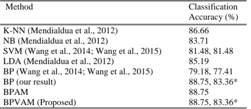
Bu tezde bir öğretici ve bir öğreticisiz olmak üzere iki yeni yapay sinir ağı metodu önerilmiştir. Öğreticili öğrenmede “değişken adaptif momentumlu geri yayılım algoritması” (DAMGY) adında yeni bir sınıflandırıcı önerilmiştir. Bu algoritma geri yayılım algoritmasının modifiye edilmiş bir halidir ve kararlı durum hataya yakınsama hızını arttırırken hata oranınıda düşürerek desen tanıma performansını arttırmayı amaçlar. Bu algoritma girişin oto korelasyon matrisinin katsayılarını kontrol eden öğrenme katsayısı tarafından kontrol edilir. Bu katsayı sayesinde ağırlıklar güncellenirken düşük hata oranı yakalanmaktadır. Algoritmanın performansını ölçmek için k-en yakın komşu (k-EYK), Naive Bayes (NB), doğrusal ayırteden analizi (DAA), Destek Vektör Makineleri (DVM), geri yayılım ve adaptif momentumlu geri yayılım algoritması (AMGY) kullanılmış ve performans, yakınsama hızı, hataların karelerinin ortalaması ve doğruluk bakımından değerlendirilmiştir.

v

Öğreticisiz öğrenmede, birçok yapay zekâ uygulamasında kullanılan kendi kendini düzenleyen harita (KDH) algoritması birçok araştırmacının ilgisini çekmektedir. Bu tezde klasik KDH algoritmasına adaptif bir öğrenme becerisi kazandıran bir algoritma önerilmiştir. Önerilen KDH algoritması değişken öğrenme katsayısı ile optimal ağırlıkları ve kazanan nöronları kısa sürede bularak klasik KDH’un dezavantajlarını yok etmektedir. Önerilen KDH algoritmasının optimum ağ ağırlıklarını bulma hızı diğer öğreticisiz algoritmalarla karşılaştırılmıştır. Ayrıca önerilen KDH algoritması klasik KDH, kendi kendini düzenleyen harita ile Gauss fonksiyonu (KDHGF) ve parametre-az kendi kendini düzenleyen harita (PAKDH) algoritmalarıyla da karşılaştırılmıştır. Önerilen KDH algoritması yakınsama hız, niceleme hızı, bulunan ağın topoloji hatası ve doğruluk kriterlerinde üstün performans gösterdiği gösterilmiştir. DAMGY ve önerilen KDH algoritmasının performansı UCI ve KEEL veritabanlarından alınan veri setleri ile de test edilmiştir.

Anahtar Kelimeler: Adaptif filtreler, iki boyutlu konveks kombinasyon, MRI, öğreticili öğrenme, yapay sinir ağı, geri yayılım, adaptif momentum, öğreticisiz öğrenme, kendi kendini düzenleyen harita (KDH), öğrenme katsayısı.

vi ABSTRACT

Ph.D THESIS

ROBUST ADAPTIVE LEARNING APPROACH OF ARTIFICIAL NEURAL NETWORKS

Alaa Ali Hameed HAMEED

THE GRADUATE SCHOOL OF NATURAL AND APPLIED SCIENCE OF SELÇUK UNIVERSITY

DOCTOR OF PHILOSOPHY IN COMPUTER ENGINEERING

Advisor: Assist. Prof. Dr. Barış KOÇER

2016, 152 Pages

Jury

Assist. Prof. Dr. Barış KOÇER Assoc. Prof. Dr. Gülay TEZEL Assoc. Prof. Dr. Sabri KOÇER

Assoc. Prof. Dr. Seral ÖZŞEN Assist. Prof. Dr. Onur İNAN

Adaptive filtering techniques are frequently used in signal processing applications. In adaptive filters, usually there is a trade-off between the steady-state mean-square error (MSE), and the initial convergence rate of the filter. This trade-off is usually controlled by the step-size. A small step-size leads to a relatively slow convergence rate with low MSE and vice versa. A new convex combination of recursive inverse (RI) and second-order RI algorithms is developed to overcome this trade-off. The new method used in system identification and noise cancellation applications. Proposed method is compared to convex combination of the normalized least-mean-square (NLMS) algorithms in terms of mean-square error (MSE) and rate of convergence. Simulations show that the proposed algorithm provides faster convergence rate with lower MSE than combined NLMS algorithms in both additive white Gaussian noise (AWGN) and additive correlated Gaussian noise (ACGN) environments.

De-noising magnetic resonance images (MRI) has recently become an interesting topic in medical diagnosis applications. Many algorithms have been proposed for this purpose. However, these algorithms usually suffer from poor performance or time consumption. In order to improve the MRI images, the proposed 1-D convex combination method extended to 2-D convex combination. The 2-D convex combination provides high performance in terms of noise removal. A de-noising experiment has been conducted on MR image that is assumed to be corrupted by an additive white Gaussian noise (AWGN) for testing purposes. Simulations show that the proposed algorithm successfully recovers the image.

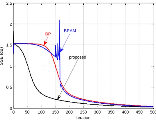
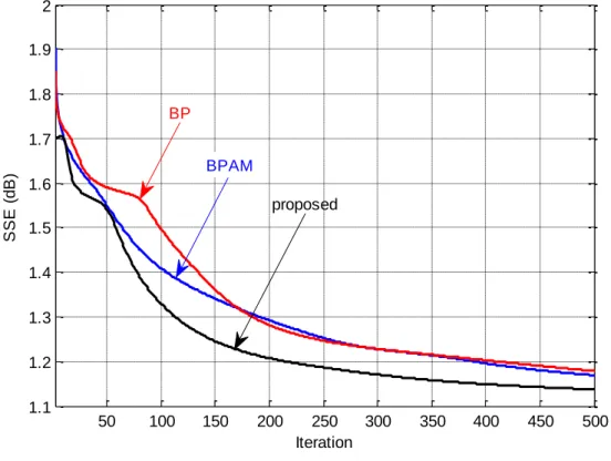
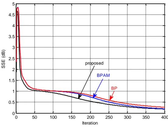
In this thesis we present two modified neural network algorithms. One of them is supervised and the other is unsupervised learning. In the supervised learning, a novel machine learning classifier of back-propagation algorithm with variable adaptive momentum (BPVAM) is proposed. The proposed algorithm is a modified version of the BP algorithm to improve its convergence behavior in both sides, accelerate the convergence process for accessing the optimum steady-state and minimizing the error misadjustment to improve the recognized patterns superiorly. This algorithm is controlled by the adaptive momentum parameter which is dependent on the eigenvalues of the autocorrelation matrix of the input. It provides low error performance for the weights update. To discuss the performance measures of the BPVAM algorithm and the other supervised learning algorithms such as K-nearest neighbours (K-NN), Naive Bayes (NB), linear discriminant analysis (LDA), support vector machines (SVM), BP, and BP with

vii

adaptive momentum (BPAM) have been compared in term of speed of convergence, sum of squared error (SSE), and accuracy.

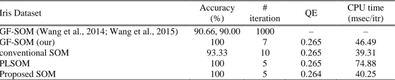
In the unsupervised learning, the self-organizing map (SOM) has attracted attention of many researchers, where it has successfully applied to a wide range of artificial intelligence applications. In this thesis, new intelligent adaptive learning of the conventional SOM algorithm is proposed. The proposed SOM overcomes the disadvantages of the conventional SOM by deriving a new variable learning rate that can adaptively achieve the optimal weights and obtain the winner neurons in a short time. Performance of the proposed SOM was compared with other unsupervised algorithms by examining the speed of finding optimum network weight update. The proposed SOM algorithm was also compared with conventional SOM, Gaussian-function with self-organizing map (GF-SOM), parameter-less self-organizing map (PLSOM) algorithms. The proposed SOM algorithm showed superiority in terms of convergence rate, quantization error (QE), topology error (TE) of preserving map and accuracy during the recognition process. The BPVAM, and proposed SOM algorithms experiments were conducted using different databases from UCI and KEEL repository.

Keywords: Adaptive filters, convex adaptive filtering, 2-D convex combination, MRI, supervised learning, neural network, back-propagation, adaptive momentum, unsupervised learning, self-organizing map (SOM), learning rate.

viii

ACKNOWLEDGMENTS

I would like to express my sincere gratitude to my supervisors Assist. Prof. Dr. Barış Koçer and Assist. Prof. Dr. Mohammad Shukri Salman for their continuous support, great guidance, endless help, knowledge and huge confidence they gave me.

I am also very grateful to Prof. Dr. Bekir Karlık for the advice and support, who has shown a large interest in my work. His stimulating motivation and valuable ideas helped me to complete this thesis. Our numerous discussions, either face-to-face or through the email, have greatly improved this work. I thank him for constructive criticism and careful revision of the text.

I would like to thank my thesis monitoring committee members Prof. Dr. Yüksel Özbay, Assoc. Prof. Dr. Gülay Tezel, Assoc. Prof. Dr. Seral Özşen for all of their guidance through this process; your discussion, ideas, and feedback have been absolutely invaluable.

I would also like to thank my colleagues and friends for all their help and collaboration. I also wish to thank my dear friend Murat Karakuş for his constant support and encouragement throughout my graduate career.

My warm regards to my amazing family, father, mother, brothers (Mohammed Ali Hameed, Ahmed Ali Hameed, Hussein Ali Hameed and Hassan Ali Hameed) and sisters for their love, support, and constant encouragement.

Alaa Ali Hameed HAMEED KONYA-2016

ix TABLE OF CONTENTS ÖZET ... iv ABSTRACT ... vi ACKNOWLEDGMENTS ... viii TABLE OF CONTENTS ... ix

LIST OF SYMBOLS AND ABBREVIATIONS ... xii

1. INTRODUCTION ... 1

1.1 Our Contributions ... 3

1.1.1 Adaptive filters ... 3

1.1.2 Artificial neural networks ... 4

1.1.2.1 Supervised learning algorithm ... 4

1.1.2.2 Unsupervised learning algorithm ... 5

1.2 Overview Of This Thesis ... 6

2. LITERATURE REVIEW ... 8

2.1 Adaptive Filters ... 8

2.2 Artificial Neural Network ... 11

2.2.1 Backpropagation (BP) algorithm ... 11

2.2.2 Self-organizing map (SOM) algorithm ... 12

3. ADAPTIVE FILTERING ... 14

3.1 Adaptive Filtering Configurations ... 15

3.1.1 System identification ... 15

3.1.2 Noise cancellation ... 16

3.2 Adaptation Algorithms ... 17

3.2.1 Normalized least-mean-square (NLMS) algorithm ... 17

3.2.2 Recursive inverse (RI) algorithm ... 18

3.2.3 Second order recursive inverse (second-order RI) algorithm ... 19

3.3 Convex Combination ... 21

3.3.1 Convex combination of RI algorithms... 21

3.3.1.1 Tracking analysis of convexly combined RI algorithms... 23

3.3.2 Convex combination of RI and second-order RI algorithms ... 27

3.3.3 2-D Convex of RI and second-order RI algorithms ... 29

x

4.1 Supervised Learning ... 33

4.1.1 Supervised learning approaches ... 34

4.1.2 Predictive model validation ... 36

4.1.3 Artificial neural network (ANN) ... 37

4.1.3.1 The biological paradigm ... 37

4.1.3.2 Basic structure of an ANN ... 38

4.1.3.3 Brief description of the ANN parameters ... 40

4.1.3.4 Neural networks neurodynamics ... 41

4.1.3.5 Neural networks architecture ... 42

4.1.3.5.1 Types of interconnections between neurons ... 42

4.1.3.5.2 The number of hidden neurons ... 42

4.1.3.5.3 The number of hidden layers ... 42

4.1.3.5.4 The perceptron ... 43

4.1.4 XOR problem with multilayer perceptron ... 44

4.1.5 Learning algorithms ... 46

4.1.5.1 The delta rule ... 47

4.1.5.2 Back-propagation (BP) algorithm ... 47

4.1.5.3 Back-propagation with adaptive filtering momentum (BPAM) algorithm ... 53

4.1.5.4 Back-propagation algorithm with variable adaptive momentum (BPVAM) algorithm ... 54

4.1.6 Statistical classification algorithms ... 55

4.1.6.1 K-NN classifier ... 55

4.1.6.2 Naïve bayes ... 56

4.1.6.3 Support vector machine... 56

4.1.6.4 Linear discriminant analysis ... 57

4.2 Unsupervised Learning ... 58

4.2.1 Unsupervised learning approaches ... 59

4.2.1.1 SOM algorithm ... 60

4.2.1.2 PLSOM algorithm ... 62

4.2.1.3 Proposed SOM algorithm ... 63

5. SIMULATION RESULTS ... 65

5.1 Convex Combination of Recursive Inverse (RI) Algorithms ... 65

xi

5.1.1.1 Convex combination of two RI algorithms ... 65

5.1.1.1.1 Additive white Gaussian noise ... 66

5.1.1.1.2 Additive correlated Gaussian noise ... 67

5.1.1.2 Convex combination of RI and second-order RI algorithms ... 69

5.1.1.2.1 Additive white Gaussian noise ... 70

5.1.1.2.2 Additive correlated Gaussian noise ... 72

5.1.2 2-D Convex combination of RI algorithms ... 75

5.1.2.1 Convex of two RI algorithms ... 75

5.1.2.2 Convex RI and second-order RI Algorithms ... 76

5.2 Back-propagation Algorithm with Variable Adaptive Momentum (BPVAM) Algorithm ... 77

5.2.1 XOR problem ... 77

5.2.2 Comparison of performances ... 79

5.2.2.1 Breast cancer dataset ... 79

5.2.2.2 Heart dataset ... 81

5.2.2.3 Heart-statlog dataset ... 82

5.2.2.4 Iris dataset ... 84

5.2.2.5 Lung-cancer dataset ... 85

5.2.2.6 MAGIC Gamma telescope dataset ... 87

5.2.2.7 Wine dataset ... 88

5.3 Proposed SOM Algorithm ... 90

5.3.1 Appendicitis dataset ... 91

5.3.2 Balance dataset ... 93

5.3.3 Wisconsin breast dataset ... 95

5.3.4 Dermatology dataset ... 97

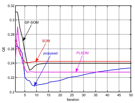
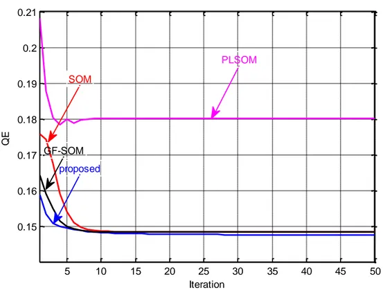
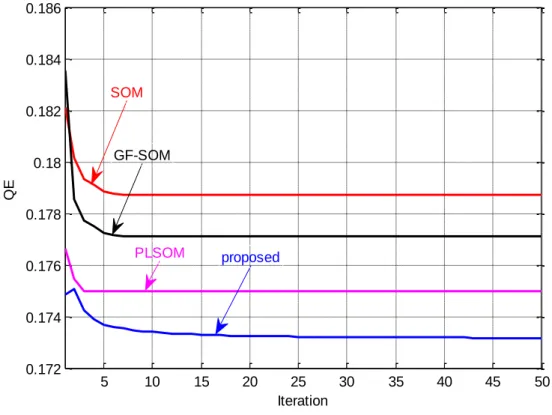
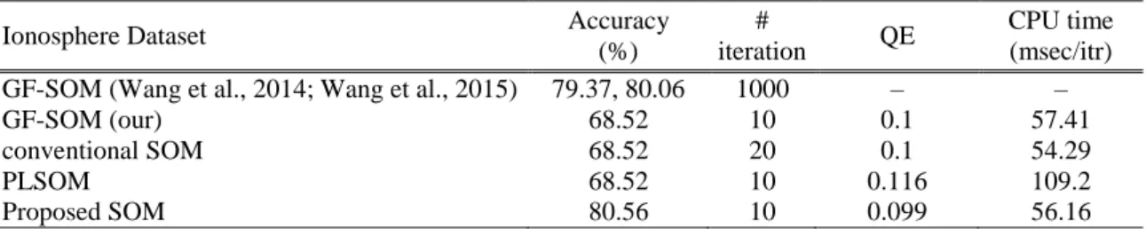
5.3.5 Ionosphere dataset... 99

5.3.6 Iris dataset ... 101

5.3.7 Sonar dataset ... 103

5.3.8 Wine dataset ... 105

6. CONCLUSION AND FUTURE WORK ... 108

REFERENCES... 110

APPENDICES ... 123

xii

LIST OF SYMBOLS AND ABBREVIATIONS

1-D 1-Dimensional

2-D 2-Dimensional

ACGN Additive Correlated Gaussian Noise

ANN Artificial Neural Networks

AR Autoregressive model

AWGN Additive White Gaussian Noise

BMU Best Matching Unit

BP Backpropagation

BPAM BP with Adaptive Momentum

BPFM BP with Fixed Momentum

BPNN Backpropagation Neural Network

BPVAM Backpropagation Algorithm with Variable Adaptive Momentum

FIR Finite Impulse Response

GF-SOM Gaussian-Function with Self-Organizing Map

IIR Infinite Impulse Response

K-NN K-Nearest Neighbours

LDA Linear Discriminant Analysis

LMS Least Mean Square

LS Least-Squares

MRI Magnetic Resonance Images

MSE Mean-Square-Error

NB Naive Bayes

NLMS Normalized Least-Mean-Square

PLSOM Parameter-Less Self-Organizing Map

QE Quantization Error

RI Recursive Inverse

RLS Recursive-Least-Squares

RZA-LLMS Reweighted Zero-Attracting Leaky-Least-Mean Square

SNR Signal-to-Noise Ratio

SOM Self-Organizing Map

xiii

SVM Support Vector Machines

TDVSS Transform Domain LMS with Variable Step-Size

TE Topology Error

ZA-LLMS Zero-Attracting Leaky Least-Mean-Square

𝐈 Identity Matrix 𝐑 Autocorrelation matrix 𝐩 Cross-correlation vector 𝐰 Weight coefficients 𝐱 Input data 𝐷 Training set 𝐸 Expectation operator 𝐸𝑢 Euler number 𝐹𝑁 False Negatives 𝐹𝑃 False Positives 𝑁 Filter length 𝑄 Covariance matrix 𝑇 Transposition operator 𝑇𝑁 True Negatives 𝑇𝑃 True Positives 𝑑 Desired response 𝑒 Estimation error 𝑓 Activation function 𝑙𝑛(. ) Natural logarithm 𝑞 Stochastic i.i.d. 𝑡 Target value 𝑣 Measurement noise 𝑦 Output 𝒉 Unknown system 𝛼 Adaptive momentum 𝛽 Forgetting factor 𝜂 Learning rate 𝜃 Threshold

xiv

𝜇 Step-size

𝜎 Width of Gaussian

𝜖 Scaling variable

1

1. INTRODUCTION

Digital filters are classified such as linear or non-linear, continuous-time or discrete-time, and recursive or non-recursive (Ozbay et al., 2003). Adaptive filtering techniques are frequently used in signal processing applications (Sayed, 2003; Sayed, 2008). The performance of adaptive filter algorithms is usually measured in terms of convergence rate and/or the minimum mean-square-error (MSE). The optimum performance of an adaptive filter is usually achieved by the Wiener filter (Haykin, 2002). However, Wiener filter requires a prior knowledge about the input signal.

While adaptive filter algorithms that does not require this prior knowledge. The performance of this algorithms is controlled by a step-size parameter that generates a trade-off between the convergence rate of the adaptive filter and its SS-MSE (Haykin, 2002; Sayed, 2003). A constant step-size parameter is used to update the filter coefficients. This step-size parameter has a critical effect on the performance of the algorithm. A relatively large step-size value provides a fast convergence but high MSE. On the other hand, a small step-size causes slow convergence with low MSE.

To overcome such a trade-off, convex combination of adaptive filters started appearing in the last decade (Arenas-Garcia et al., 2006; Mandic et al., 2007; Kosat and Singer, 2009; Azpicueta-Ruiz et al., 2008; Trump, 2009a). Convex combination of adaptive filter has provided an improved performance in both stationary and non-stationary environments (Zhang and Chambers, 2006). The convex combination is usually constructed by two adaptive filters; one of them provides fast convergence with high output steady-state error and the other has slow convergence with low MSE (Martinez-Ramon et al., 2002). The schematic diagram of the convex combination of adaptive filters is shown in Fig. 2.1.

Therefore, a combination of such two systems would provide us, in a way, a solution of such trade-off. This solution is done by extracting out the faster converging part and the lower MSE part from the two filtering algorithms. By this the filter will provide a performance with fast convergence and low error.

A 2-Dimensional (2-D) adaptive filter is an extension of 1-D adaptive filters which deals with two dimensional signals (i.e., images) (Hadhoud and Thomas, 1998). One of the most attracting applications of such algorithms is image de-noising.

Artificial neural networks is an interesting research that is well-known in the area of machine learning and has provided the best solutions to many problems.

2

Currently it attracts more and more attendance in artificial intelligence. In general, the Artificial neural networks try to model useful high-level abstractions, learning hierarchies of concepts, and multiple-layer architectures for better data representations. Artificial neural networks is capable of learning complex abstractions and it is known to be especially useful for problems with high-dimensional input, such as speech and image recognition.

Backpropagation neural network (BPNN) is a supervised machine learning that has attracted the attention of many researchers in a wide range of applications. BPNN has high capability to solve complex problems that cannot be solved using traditional machine learning techniques (Karlik, 2014). There are many BPNN applications on marketing (Iseri and Karlik, 2009; Chiang et al., 2006), bioinformatics (Karlik, 2013), medicine (Behram et al., 2007; Karlik and Cemel, 2012), engineering (Dvir et al., 2006; Karlik, 2000), and others (Karlik et al., 1998; Lee et al., 2005). Unfortunately, it has a couple of obstacles that usually restrict its algorithm performance; the slow convergence and the high steady-state error. To overcome these obstacles, the momentum technique have been proposed, where it can speed up the convergence rate and decrease the steepest descent error (Yu et al., 1993; Yu and Liu, 2002; Shao and Zheng, 2009), efficiently.

Self-organizing map (SOM) as an unsupervised learning algorithm attracts many researchers. It can be applied in various applications such as clustering, image recognition, and sound recognition (Kohonen, 1990; Kohonen et al., 1996; Vesanto and Alhoniemi, 2000). SOM projects the input samples from high dimensional space to the low dimensional space (Kohonen, 1982; Kohonen, 2001). The architecture of SOM is simply consists of an input layer and an output layer with highly interconnection between each other where each connection is associated with a weight. The output is organized as a two dimensional grid of neurons, where the data visualization of the output is implemented during the learning process.

SOM algorithm does not require the knowledge of the target output in the recognition process (Mukherjee, 1997). The conceptual idea is that each input vector is multiplied by the weight vectors to calculate the distances. Furthermore the map nodes output must be the same weight vectors (Kohonen, 1989; Song and Hopke, 1996; Kim et al., 2002; Hoffmann, 2005; Marini et al., 2005; Bianchi et al., 2007). The winner output node is determined by the shortest distance between the input vector and output nodes. The winner weights node are updates for each input (Rojas, 1996; Astel et al.,

3

2007). The clustering inputs depending on the similarity of the input features (Fonseca et al., 2006). The time consumption of training depends on dataset size and whether it can reach the optimum weights.

1.1 Our Contributions

In this work we have proposed different algorithms; we have proposed a new convex combination RI adaptive filter and we derive its tracking analysis; for artificial neural networks we have proposed a new backpropagation algorithm called BPVAM, and a new SOM algorithm.

1.1.1 Adaptive filters

In order to overcome the trade-off in the field of adaptive filtering, various variable step-size LMS-type algorithms have been developed. Recently, Ahmad et al. (2011) have proposed a new recursive inverse (RI) adaptive algorithm. This algorithm has shown great performance compared to different adaptive algorithms with less or comparable computational complexity (Ahmad et al., 2010b). It has shown robust performance in impulsive noise and non-stationary environments (Ahmad et al., 2012; Ahmad et al., 2013b). However, the trade-off between the convergence rate and the MSE is not radically solved.

In this work, we propose a new RI convexly combined adaptive filtering algorithms which provides a very high performance, in terms of convergence rate and SS-MSE, compared to the other proposals. The new convex combination of RI algorithms is to extract the fast convergence and low MSE properties of two adaptive filters and combine their performances. The tracking performances of the convexly combined RI algorithms have been discussed theoretically and experimentally. It shows that the derived theoretical SS-MSE of the convexly combined RI algorithm is in match with the experimental one.

The performance of proposed convex combinations has compared to various adaptive algorithms and others convex combinations that shown in the literature (see Chapter 3):

1. Normalized least-mean-square (NLMS) algorithm. 2. Recursive inverse (RI) algorithm.

4 3. Second order RI Algorithm.

4. Convex of Two NLMS Algorithms. 5. Convex of Two RI Algorithms.

6. Convex RI and second order RI Algorithms.

In additive white Gaussian noise (AWGN) and additive correlated Gaussian noise (ACGN) environments in the settings of system identification, and noise cancellation.

Simulation results show that the new combinations highly outperforms other algorithm in terms of both MSE and convergence rate. Furthermore, the 2-D version of the algorithm has shown high performance in image de-noising.

1.1.2 Artificial neural networks

The proposed neural networks algorithms are BPVAM which is for supervised learning, and new SOM algorithm for unsupervised learning.

1.1.2.1 Supervised learning algorithm

The conventional BP algorithm has a couple of obstacles that usually limit its performance; the slow convergence and the high steady-state error. To overcome these obstacles, the new variable adaptive momentum technique has been proposed, where it can speed up the convergence rate and decrease the steepest descent error SSE, efficiently.

This momentum has been proposed as a learning rate in (Ahmad et al., 2011; Ahmad et al., 2010a; Ahmad et al., 2013a; Hameed et al., 2014) and has been used simply in various adaptive filtering applications successfully. This proposed adaptive momentum is characterized by two parameters (𝜆, 𝛽) providing lower computational cost and more robustness in various applications. It also shows better performance deservedly over the conventional BP and BPAM algorithms in terms of speed of convergence, SSE and accuracy.

To prove our claim, the performance of the proposed BP algorithm based on a variable adaptive momentum, shortly called BPVAM, are compared to different supervised machine learning techniques that take place in the literature (see Chapter 4):

5 2. Naive Bayes (NB).

3. Linear discriminant analysis (LDA). 4. Support vector machines (SVM). 5. Back-propagation (BP).

6. Back-propagation with adaptive momentum (BPAM).

For this purpose, the BPVAM and the other algorithms were applied on a benchmark-XOR problem and various datasets such as breast cancer, heart, heart-statlog, iris, lung-cancer, MAGIC gamma telescope, and wine datasets recorded at UCI repository in order to compare their performance. The results show that the performance of the BPVAM algorithm is better than the others.

1.1.2.2 Unsupervised learning algorithm

The major problem with SOMs is that they are very computationally expensive which is a major drawback since as the dimensions of the data increases, dimension reduction visualization techniques become more important, but unfortunately then time to compute them also increases. For calculating the input features similarity map, the more neighbors you use to calculate the distance the better similarity map you will get, but the number of distances the algorithm needs to compute increases exponentially.

In this thesis a new adaptive learning rate of decreasing functions. The proposed SOM algorithm overcomes many disadvantages of conventional SOM algorithm. It needs less implementation time (fast convergence), obtains low Quantization Error (QE) and better Topology Error (TE) preserving map during the recognition process.

Experiments also showed that the proposed algorithm is able to recognize more features and getting a higher accuracy compared to different unsupervised machine learning techniques that shown in the literature (see Chapter 4):

1. Conventional self-organizing map (SOM) algorithm.

2. Gaussian-function with self-organizing map (GF-SOM) algorithm. 3. Parameter-less self-organizing map (PLSOM) algorithm.

In this thesis, the new unsupervised learning algorithm is compared with conventional SOM, GF-SOM and PLSOM algorithms using different criteria such as QE, TE, CPU time and accuracy. Extensive experiments are conducted to evaluate the performance of proposed algorithm using different well-known datasets such as Appendicitis, Balance, Wisconsin breast, Dermatology, Ionosphere, Iris, Sonar and

6

Wine datasets from UCI and KEEL repositories. The new SOM outperforms the other algorithms in terms of the used criteria as shown in the results.

1.2 Overview Of This Thesis

This thesis is organized as follows. Introduction and our contributions are outlined in Chapter 1. Chapter 2 provides a literature review about the well-known adaptive filters and their significance, where some adaptive filtering algorithms have been presented by many researchers for better learning and adapting rates. Also, machine learning in supervised and unsupervised learning have presented. BP neural network, and SOM algorithms have presented with some of their variants.

Chapter 3 introduces the adaptive filters and their mechanism, system identification and noise cancellation configurations, some adaptive filtering algorithms, the proposed convex combinations including the one-dimensional (1-D), and two-dimensional (2-D) convexly combined RI algorithms.

In Chapter 4, machine learning in supervised and unsupervised learning are introduced. The supervised BP neural network and the unsupervised SOM learning algorithms are briefly described. In addition the proposed BPVAM, and proposed SOM algorithms derivations are proved.

In Chapter 5, in section one, the proposed convex combinations of RI algorithms compared to the performance of convex NLMS algorithms are discussed. In simulation results the combinations performance were investigated in terms of the MSE and convergence rate for system identification, and noise cancellation settings, in both additive white Gaussian noise (AWGN) and additive correlated Gaussian noise (ACGN) environments. In section two, the performance measures of proposed BPVAM algorithm and the other supervised learning algorithms such as K-nearest neighbours (K-NN), Naive Bayes (NB), linear discriminant analysis (LDA), support vector machines (SVM), BP, and BP with adaptive momentum (BPAM) are compared in terms of speed of convergence, sum-of-squared-error (SSE), and accuracy by implementing benchmark XOR-problem and seven datasets from UCI repository. In the last section, the proposed SOM algorithm was also compared to the conventional SOM, GF-SOM and PLSOM algorithmsin terms of convergence rate, quantization error (QE), topology error (TE) preserving map and accuracy during the recognition process. Extensive experiments were conducted using eight different datasets from UCI and KEEL

7 repository.

8

2. LITERATURE REVIEW

This chapter will provide overviews about the adaptive filters, their problems and development stages in general. Also, the artificial neural networks (ANN), its architecture, and their advantages and disadvantages will present.

2.1 Adaptive Filters

Performing common processing operations on a sequence of data can be considered as filtering the raw data (Canan et al., 1998). A digital filter with fixed coefficients can be designed by using well defined proporties. However, in some situations, where the specifications are not available or time-varying, a filter that updating the coefficients with time is required which is called as an adaptive filter. Adaptive filtering has shown a great interest by researchers during the last decades. This interest is due to those vast application areas of adaptive filters (Muneyasu et al., 1998; Haykin, 2002; Sayed, 2003; Salman, 2014; Gwadabe and Salman, 2015; Ma et al., 2015).

LMS algorithm is one of the well-known adaptive filtering techniques which has been used to solve many problems. However, the performance of an adaptive filter is usually controlled by some parameters that usually generate a trade-off between the convergence rate and SS-MSE. Since the LMS algorithm is a gradient descent based algorithm, a constant step-size parameter is used to update the filter coefficients. This step-size parameter has a critical effect on the performance of the algorithm. A large step-size value provides a fast convergence but a high MSE where a small step-size causes slow convergence with low MSE. This trade-off can be set in the favor of both increase in the convergence rate and decrease in misadjustment for the best performance by using a variable step-size (Aboulnasr and Mayyas, 1997; Turan and Salman, 2014).

The NLMS algorithm has been proposed to improve the performance of the traditional LMS algorithm (Haykin, 2002). The NLMS algorithm provides a fast convergence rate, and achieves a minimal steady-state error by normalizing the step-size by the power of the input. Shin et al., (2004) have developed a variable step-size affine projection algorithm to improve the convergence rate with lower misadjustment at early stages of adaptation.

9

performance in adaptive filtering, which outperforms the LMS algorithm and its versions (Maouche and Slock, 2000; Wang, 2009; Eksioglu and Tanc, 2011). The RLS algorithm can keep the output performance in the steady-state on improving over time. In the case of the least-squares (LS) algorithms, the performance is controlled by the forgetting factor with a value close to unity to obtain the convergence and stability of the algorithm at the same time.. A major drawback of the RLS algorithm is its high computational complexity (Haykin, 2002).

Ahmad et al., (2011) has proposed a new RI adaptive filtering algorithm that showed better performance compared to the transform domain LMS with variable step-size (TDVSS) in terms of the convergence rate, and it is very comparable to the RLS algorithm, with lower computational complexity than RLS algorithm by avoiding the inversion of the autocorrelation matrix. Ahmad et al., (2010b) used the second-order estimates of the correlations, the second-order RI algorithm has provided MSE performance that cannot be attained using the TDVSS algorithm. It has shown robust performance in impulsive noise and non-stationary environments (Ahmad et al., 2012; Ahmad et al., 2013b). However, the trade-off between the convergence rate and the MSE is not radically solved.

In the last decade, a convex combination of adaptive filtering algorithms has been frequently used to overcome this trade-off (Kozat and Singer, 2000; Arenas-Garcia et al., 2003; Arenas-Garcia et al., 2005; Arenas-Garcia et al., 2006; Azpicueta-Ruiz et al., 2008; Silva and Nascimento, 2008; Trump, 2009a; Trump, 2009b; Azpicueta-Ruiz et al., 2010). The main idea behind these proposals is to extract the fast convergence and low MSE properties of two adaptive filters and combine their performances. However, most of these proposals still converge to a relatively high MSE. The convex scheme consists of combining two adaptive filters. One possibility is depicted in Fig. 2.1. The output and error estimates of the adaptive filters are combined using the parameter 𝜆(𝑛). Mandic et al., (2007) proposed a collaborative adaptive learning algorithm using hybrid filters. They combined two different adaptive filters in order to attain lower MSE with high convergence rate. However, the combined performance of their proposed algorithm cannot exactly track the learning curves of both filters. Trump (2009b) discussed the tracking performance of a combination of two NLMS adaptive filters. In that paper, the combiner can track the learning curves of the combined filters.

10

Figure 2.1. The block diagram of the convex combination of adaptive filters

Salman et al., (2015) proposed a new convex combination of two different algorithms as attracting leaky least-mean-square (ZA-LLMS) and reweighted zero-attracting leaky-least-mean square (RZA-LLMS) algorithms in sparse system identification setting. The performances of the aforementioned algorithms has been tested and compared to the result of the new combination. It showed that the proposed algorithm has a good ability to track the MSD curves of the other algorithms under a various noise environments.

A 2-Dimensional (2-D) adaptive filters is an extension of 1-D adaptive filters which deals with two dimensional signals (i.e., images) (Hadhoud and Thomas, 1998). One of the most attracting applications of such algorithms is image de-noising. There are many 2-D adaptive algorithms such as: OBA, OBAI, TDBLMS, TDLMS, and TDBLMS (Mikhael and Wu, 1989; Mikhael and Ghosh, 1992; Hadhoud and Thomas, 1998; Wang and Wang, 1998). Two-dimensional least-mean-square (TDLMS) updates its coefficients in horizontal and vertical directions on a 2-D plane. Even though the 2-D LMS algorithm has shown good performance in image de-noising systems, its

𝜆(𝑛) 𝑦2(𝑛) 𝑒2(𝑛)

-+

+

+

11

performance still poor when the signal-to-noise ratio (SNR) is relatively low.

Magnetic resonance image (MRI) de-noising is one of the most interesting applications in adaptive filters techniques, especially, if the SNR is relatively low (Phatak et al., 2011) or the noise model is complicated. For instance, if the MRI data is corrupted by Rician noise from the measurement process, this will reduce the accuracy of any automatic analysis (Mustafa et al., 2012). The challenge, here, is to remove such noise by segmentation, classification and registration (Chang et al., 2011). There are many applications to denoising in the MRI such as, adaptive multi-scale data condensation (Ray et al., 2012) total variation and local noise estimation (Varghees et al., 2012) and adaptive non-local means filtering (Kang et al., 2013).

However, these algorithms usually suffer from poor performance or time consumption. Hameed et al., (2014) proposed a 2-D version convex combination of recursive inverse algorithms (RI) algorithm that provides fast convergence at the beginning to save time and then provides high performance in terms of noise removal. The de-noising experiment has been conducted on MR image that is assumed to be corrupted by an additive white Gaussian noise (AWGN). Simulations showed that the proposed algorithm successfully recovers the image.

2.2 Artificial Neural Network

Backpropagation (BP) neural networks, and Self-organizing map (SOM) are common neural network algorithms, they provide high performances in solve many different problems in a wide range of applications as shown in this literature.

2.2.1 Backpropagation (BP) algorithm

BP artificial neural networks algorithm is an interesting topic which has attracted many researchers in various domains (Karlik et al., 1998; Karlik, 2000; Lee et al., 2005; Chiang et al., 2006; Dvir et al., 2006; Behrman et al., 2007; Iseri and Karlik, 2009; Karlik and Cemel, 2012; Karlik, 2013). However, it has a couple of obstacles that usually restrict its algorithm performance; the slow convergence and the high steady-state error. In order to speed up the convergence rate and decrease the steepest descent error, the momentum technique has been proposed (Yu et al., 1993; Yu and Liu, 2002; Shao and Zheng, 2009). Many versions of momentum have been proposed and trained

12

in different applications (Qiu et al., 1992; Istook and Martinez, 2002). The BP with fixed momentum (BPFM) has been proposed by adding a momentum term to the conventional BP weight update equation (Rumelhart and McClelland, 1986; Rumelhart et al., 1988) which can speed up learning by reaching optimal steady-state error in short time. Whereas, the fixed momentum is supposed to be constant within the range of [0,1]. Unfortunately, when the fixed momentum is in the direction of the negative gradient which is in an opposing direction to the previous update, it may cause the weight to be arranged the slope of the error surface instead of down the slope as target. The fixed momentum has also been extended to adaptive momentum by superiorly adapting itself along with iterations, achieving optimal convergence speed in the BP implementation. The adaptive momentum can update itself iteratively and automatically during the iteration process and depending on the prediction of the output error (Wu et al., 2002; Wu and Xu, 2002).

Yu and Liu (2002) proposed a new acceleration technique of BP algorithm by deriving adaptive learning rate and momentum coefficient. The proposed adaptive parameters are adjusted iteratively to access the optimum weight vectors in a short time of process. Where, the new BP proved superior convergence compared to other competing methods.

Shao and Zheng (2009,2011) have proposed a back-propagation with adaptive momentum (BPAM) which provides better performance than the conventional BP algorithm in terms of both convergence rate (decreasing time of convergence) and SSE. In their study, the momentum is updating itself iteratively by multiplying the current weights with the previous weights. If the momentum coecients are less than zero, they are denied as positive value to accelerate learning by updating momentum. Otherwise the momentum is considered as zero to maintain the error downhill.

2.2.2 Self-organizing map (SOM) algorithm

SOM which is most common unsupervised algorithm used in artificial neural networks has been proposed by (Kohonen, 1990). SOM used to solve many problems of different applications (Kaski et al., 1998; Tamukoh et al., 2004). It maps the input data from high dimensional input vector to low dimensional maps according to the features relations between the input data. The algorithm competitive layer used to learn clustering the input vectors. SOM algorithm is suffers from the time consumption of

13

training. Training time depends on dataset size and whether the algorithm can reach the optimum weights and the topology preservation.

Many versions of the SOM have been proposed to improve the vector quantization and the topology preservation performances (Chi and Yang, 2006; Wong et al., 2006; Brugger et al., 2008; Chi and Yang, 2008; Gorgonio and Costa, 2008; Yen and Wu, 2008; Cottrell et al., 2009; Arous and Ellouze, 2010; Tasdemir et al., 2011; Appiah et al., 2012; Ayadi et al., 2012; Yang et al., 2012). In (Brugger et al., 2008), authors proposed a new way that can detect the cluster automatically by applying the cluster algorithm (Bogdan and Rosenstiel, 2001) to the SOM.

Chi and Yang (2006) proposed a hybrid clustering by combining SOM, and the ant K-means algorithm which is a meta-heuristic method that has been used to investigate the optimum solutions of many problems. So, the ant K-means algorithm used to guide the K-means algorithm to the place the objects with high probabilities depending on the characteristic of pheromone updating. The SOM and ant K-means algorithm has high performance compared to the conventional SOM algorithm, and some clustering methods.

Another improvement proposed by (Tasdemir et al., 2011), which is demonstrated that the neurons of SOM can be clustered hierarchically depending on the density without needing the distance dissimilarity. In addition, the Gaussian-function with self-organizing map (GF-SOM) algorithm has been widely used in many applications as a neighborhood function.

To overcome the limitation of conventional SOM, Berglund & Sitte proposed a new SOM called the Parameter-Less self-organizing map (PLSOM) algorithm (Berglund and Sitte, 2006). Their algorithm calculates the local quadratic fitting error instead of using the well-known neighbourhood size and learning parameters as in the conventional SOM algorithm. The problem with PLSOM algorithm is in the initial weight distribution which suffers from over-reliance and over-sensitivity to outliers. This suffering continues even after a period of processing time (Berglund, 2010).

Yamaguchi et al., (2010) proposed an adaptive hierarchical competitive network layer of SOM algorithm based on Tree-Structured. The proposed algorithm adapts automatically to detect the optimum number of neurons, by adding or deleting the map neurons using means error and frequency techniques.

14

3. ADAPTIVE FILTERING

Adaptive filtering has been implemented to overcome the limitations of the conventional static filters, where the adaptive filter can deal with unknown or time varying input signals in a various noise environments (Diniz, 1997). They have been used in different applications such as: system identification (Glentis et al., 1999), channel equalization/identification and interference suppression in communications systems (Madhow and Honig, 1994; Gesbert and Duhamel, 2000), and acoustic echo cancellation (Gay and Benesty, 2000). The main idea of filter adaptation is the output signals of the filter depends on the weight coefficient vectors, that adjust itself iteratively with time processing to minimize the error of estimation between filter output and desired output. Fig. 3.1 illustrates the main diagram of an adaptive filter. It is shown in the figure how to remove noise using adaptive filters, where 𝑦(𝑛) is the filter output, 𝑑(𝑛) is the desired response and 𝑒(𝑛) is the estimation error of the adaptive filter for time iteration 𝑛.

Adaptive filters classified as; finite impulse response (FIR), and infinite impulse response (IIR). IIR filters are beyond the scope of this thesis. The output of adaptive FIR filter is obtained linearly by combining the present and past input signal samples 𝑁 − 1, where 𝑁 is the number of the filter coefficients. Adaptive FIR filter is preferred over adaptive IIR filter because of its robustness and simplicity. Moreover, FIR filters have been used in many practical applications such as: channel estimation in communications systems (Breining et al., 1999).

Figure 3.1. Block diagram of the statistical filtering problem

Desired response 𝑑(𝑛) Input 𝐱(𝑛)

-

+

𝞢

15 3.1 Adaptive Filtering Configurations

Two adaptive filtering configurations are presented in this thesis. One application is system identification and the other is noise cancellation. Different adaptive algorithms will be tested using this applications in additive white Gaussian noise (AWGN) and additive correlated Gaussian noise (ACGN) environments.

3.1.1 System identification

This configuration has been used in several areas. The system identification is necessary for many applications such as: identification of the acoustic echo path in acoustic echo cancellation (Dogancay and Tanrikulu, 2001), channel identification in communications systems (Gesbert and Duhamel, 2000). The adaptive filter is capable to obtain a best fit of a linear model for an unknown system with a time varying model. The unknown system and adaptive filter are fed simultaneously by the same input signal, and the output of the unknown system added to measurement noise 𝑣(𝑛) to provide the desired response signal of the adaptive filter 𝑑(𝑛), where 𝑑(𝑛) = 𝒉𝑇𝐱(𝑛) + 𝑣(𝑛), 𝒉 is the optimal filter coefficient vector (unknown system). Fig. 3.2 depicts the system identification configuration.

Figure 3.2. System identification configuration 𝑦(𝑛) 𝑣(𝑛) 𝐱(𝑛)

-

+

+

16

where 𝐱(𝑛), 𝑣(𝑛), 𝑦(𝑛), and 𝑒(𝑛), are the input signal, the measurement noise, adaptive filter output signal and the irreducible error, respectively.

3.1.2 Noise cancellation

This configuration is used to eliminate noise by passing the received signal through the configuration using adaptive algorithm. Static filters need to have prior knowledge about the characteristics of the input signal or noise to estimate the desired information. While, the adaptive filters do not require prior knowledge about input signal. Noise cancellation is applied in radio communications and mobile phones, because those are affected from high-noise signals. The adaptive noise cancellation is depicted in Fig. 3.3.

Figure 3.3. Noise cancellation configuration

The desired response 𝑑(𝑛) includes the input 𝐱(𝑛) and an uncorrelated noise 𝑣(𝑛). A second input 𝑣′(𝑛) used as a noise to feed the adaptive filter which is uncorrelated with 𝑣(𝑛) and independent of 𝐱(𝑛) so that it can extract the desired information. The filter coefficients of adaptive algorithm 𝐰(𝑛) adjust themselves automatically to reduce the error 𝑒(𝑛) between 𝑦(𝑛) and 𝑑(𝑛), and obtain the desired signal. 𝑦(𝑛) 𝑣′(𝑛)

-

+

17 3.2 Adaptation Algorithms

In this section, some adaptive filters are reviewed. The first algorithm is the normalized least-mean-square (NLMS) proposed in (Haykin, 2002), the second is the recursive inverse (RI) by (Ahmad et al., 2011), and the last one is the second-order recursive inverse (second-order RI) by (Ahmad et al., 2013b). These algorithms have been used in diverse adaptive filtering applications.

3.2.1 Normalized least-mean-square (NLMS) algorithm

The least-mean-square (LMS) algorithm is a widely used adaptive algorithm (Bouboulis and Theodoridis, 2010). It is characterized by its simplicity, robustness and low cost (Haykin, 2002). This adaptive algorithm is based on the gradient descent method of the cost function (𝐽(𝑛) = 𝑒2(𝑛)). The weight update equation of LMS algorithm is derived as,

𝐰(𝑛) = 𝐰(𝑛 − 1) + 𝜇𝐱(𝑛)𝑒(𝑛) (3.1)

Where 𝜇 is the step-size, that controls the convergence rate and the stability of the algorithm.

The LMS algorithm adjusts the tap weights vector in a recursive manner until obtaining the optimum weights vector to access minimum error on the required signal using (3.1). The step size is constant in the range of,

0 < 𝜇 < 2

𝜆_𝑚𝑎𝑥 (3.2)

Where 𝜆𝑚𝑎𝑥 is the input autocorrelation matrix 𝐑 with largest eigenvalue, used to guarantee the stability. The trace of 𝐑 (sum of the eigenvalues) is used instead of 𝜆_𝑚𝑎𝑥. Therefore, the value of step-size is within 0 < 𝜇 < 2

𝑡𝑟𝑎𝑐𝑒 (𝐑). The trace (𝐑) = ‖𝐱(𝑛)‖2 _{is related to the power of the 𝐱(𝑛). The well-known step size is obtained as;}

0 < 𝜇 < 2

18

The step-size 𝜇 is inversely proportional to the power of the input signal. Accordingly, when the power of the input is high, the step size is imposed to a small value, on the other hand, when the power of the input is low the step size becomes large. This relationship enables normalizing the step-size of the LMS algorithm according to the input signal power. The normalized step-size provides a useful LMS-type algorithm, commonly known as normalized LMS (NLMS) algorithm (Haykin, 2002).

The NLMS algorithm with normalized step-size term updates the weights vector as,

𝐰(𝑛) = 𝐰(𝐧 − 𝟏) + 𝜇

𝐱𝑇_{(𝑛)𝐱(𝑛) + 𝜖}𝐱(𝑛)𝑒(𝑛) (3.4)

Where the step-size is in the range [0,2]. The importance of normalizing the step size is improving the convergence behavior in the NLMS algorithm. So the algorithm becomes powerful in non-stationary applications like speech recognition. In addition, the speed of convergence is improved to achieve the minimum steady-state MSE quickly (Azpicueta-Ruiz et al., 2010).

3.2.2 Recursive inverse (RI) algorithm

Any stationary discrete-time stochastic process can be expressed as:

𝐱(𝑛) = 𝑢(𝑛) + 𝑣(𝑛) (3.5)

Where 𝑢(𝑛) is the desired signal and 𝑣(𝑛) is the noise process. Removing noise from 𝐱(𝑛) is a challenge in many signal-processing applications.

Many adaptive algorithms have been used to update the coefficients of the filter shown in Fig. 3.1. In the recently proposed adaptive RI algorithm, the autocorrelation matrix is recursively estimated and not its inverse. The weight-updated equation of the RI is:

19

Where 𝑛 is the time parameter (𝑛 = 1,2, … ), 𝐰(𝑛) is the filter weight vector at time 𝑛 with length 𝑁 , 𝐈 is an 𝑁 × 𝑁 identity matrix, 𝜇(𝑛) is the variable step size, 𝐑(𝑛) is the autocorrelation matrix of the tap-input vector, and 𝐩(𝑛) is the cross-correlation vector between the tap-input vector and desired response of the adaptive filter. The correlations of the tap-input vector and the desired response are recursively estimated as:

𝐑(𝑛) = 𝛽𝐑(𝑛 − 1) + 𝐱(𝑛)𝐱𝑇(𝑛) (3.7)

𝐩(𝑛) = 𝛽𝐩(𝑛 − 1) + 𝑑(𝑛)𝐱(𝑛) (3.8)

Where 𝛽 is the forgetting factor, which is usually selected very close to unity, and the step size μ(n) is given as:

𝜇(𝑛) = 𝜇0

1 − 𝛽𝑛 𝑤ℎ𝑒𝑟𝑒 𝜇0 < 𝜇𝑚𝑎𝑥 (3.9)

Where 𝜇_𝑚𝑎𝑥 < 2

𝜆𝑚𝑎𝑥(𝐑(𝑛)) and 𝜆𝑚𝑎𝑥(𝐑(𝑛)) is the maximum eigenvalue of 𝐑(𝑛).

3.2.3 Second order recursive inverse (second-order RI) algorithm

In order to improve the performance of the RI algorithm, a second-order RI estimate of the correlations with the same updated equation as in (3.6) can be used:

𝐑(𝑛) = 𝛽1𝐑(𝑛 − 1) + 𝛽2𝐑(𝑛 − 2) + 𝐱(𝑛)𝐱𝐓(𝑛) (3.10)

𝐩(𝑛) = 𝛽₁𝐩(𝑛 − 1) + 𝛽₂𝐩(𝑛 − 2) + 𝑑(𝑛)𝐱(𝑛) (3.11)

By selecting 𝛽₁ = 𝛽₂ = 1

2𝛽, the computational complexity of the second-order RI will be comparable to that of the first-order RI algorithm. Taking the expectation of Eq. (3.10) gives:

20 𝐑̅(𝑛) =1

2𝛽1𝐑̅(𝑛 − 1) + 1

2𝛽2𝐑̅(𝑛 − 2) + 𝐑𝐱𝐱 (3.12)

Where 𝐑_𝐱𝐱 = 𝐸{𝐱(𝑛)𝐱𝑇(𝑛)} and 𝐑̅(𝑛) = 𝐸{𝐑(𝑛)}. After calculating the transfer function of Eq. (3.12), its poles are:

𝑧₁ =1

4(𝛽 − √𝛽2+ 8𝛽)

(3.13)

𝑧₂ = 1

4(𝛽 + √𝛽2+ 8𝛽)

Where 𝑧₁ and 𝑧₂ have magnitudes of less than unity if 𝛽 < 1. Solving Eq. (3.12) with the initial conditions 𝐑̅(−2) = 𝐑̅(−1) = 𝐑̅(0) = 0 yields:

𝐑̅(𝑛) = ( 1 𝛽 − 1+ 𝛼1𝑧1 𝑘_{+ 𝛼} 2𝑧2𝑘) 𝐑𝐱𝐱 (3.14) Where 𝛼₁ = 𝛽 − 𝑧2 (1 − 𝛽)(𝑧₂− 𝑧₁) (3.15) 𝛼₂ = 𝛽 − 𝑧1 (1 − 𝛽)(𝑧₂− 𝑧₁) Letting 𝛾(𝑛) = 1 𝛽 − 1+ 𝛼1𝑧1 𝑛_{+ 𝛼} 2𝑧2𝑛 (3.16)

The variable step size of the second-order RI algorithm is then:

𝜇(𝑛) = 𝜇0

21

Where 𝜇₀ and 𝛾(𝑛) are defined in Eqs. (3.9) and (3.16), respectively. This variable step size enables us to reach a low MSE that cannot to be attained by the NLMS or the first-order RI algorithm.

3.3 Convex Combination

In this section, different RI convex combinations such as convex combination of RI algorithms, convex combination of RI and second-order RI algorithms, and 2-D convex of RI and second-order RI algorithms have been proposed to improve the performance of the adaptive filters.

3.3.1 Convex combination of RI algorithms

Consider the combination of two adaptive filters in noise cancelation setting which has been recently proposed in (Ma et al., 2015), as shown in Fig.3.4. Starting by the update equation of the RI.

Figure 3.4. Convex combination of two adaptive filters for a noise cancelation setting 𝑒2(𝑛)

-+

+

+

22

𝐰𝑖(𝑛) = [𝐈 − μ𝑖(𝑛)𝐑𝑖(𝑛)]𝐰𝑖(𝑛 − 1) + μ𝑖(𝑛)𝐩𝑖(𝑛) (3.18)

Where 𝑛 is the time index (𝑛 = 1,2, … ), 𝐰_𝑖(𝑛) is the ith _{filter weight vector at} time 𝑛 with length 𝑁 (𝑖 = 1, 2), I is an 𝑁 × 𝑁 identity matrix, μ𝑖(𝑛) is the ith variable step-size, 𝐑_𝑖(𝑛) is the ith _{autocorrelation matrix of the tap-input vector and 𝐩}

𝑖(𝑛) is the ith cross-correlation vector between the tap-input vector 𝐱(𝑛) and desired response 𝑑(𝑛) of the adaptive filter. The correlations are recursively estimated as the following,

𝐑_𝑖(𝑛) = 𝛽𝐑𝑖(𝑛 − 1) + 𝐱(𝑛)𝐱𝑇(𝑛) (3.19)

𝐩_𝑖(𝑛) = 𝛽𝐩_𝑖(𝑛 − 1) + 𝑑(𝑛)𝐱(𝑛) (3.20)

Where 𝛽 is the forgetting factor with a value close to unity.

μ_𝑖(𝑛) = μ0

1 − 𝛽𝑛 𝑤ℎ𝑒𝑟𝑒 μ0 < μ𝑚𝑎𝑥 (3.21)

Where μ𝑚𝑎𝑥 < 2

𝜆𝑚𝑎𝑥(𝐑𝑖(𝑛)) and 𝜆𝑚𝑎𝑥(𝐑𝑖(𝑛)) is the maximum eigenvalue of 𝐑_𝑖(𝑛).

The error of each individual filter is formulated as

𝑒𝑖(𝑛) = 𝑑(𝑛) − 𝐰𝑖𝑇(𝑛 − 1)𝐱(𝑛) (3.22)

And the desired response is;

𝑑(𝑛) = 𝐱(𝑛) + 𝜈(𝑛) (3.23)

Where 𝜈(𝑛) is the measurement noise. The outputs of the two adaptive filters can be combined according to (Arenas-Garcia et al., 2006; Azpicueta-Ruiz et al., 2008), by the following equation,

23

where 𝑦_𝑖(𝑛) = 𝐰_𝑖𝑇(𝑛 − 1)𝐱(𝑛) and convex combination parameter, 𝜆(𝑛) is given by,

𝜆(𝑛) = 𝐸[(𝑑(𝑛) − 𝑦2(𝑛))(𝑦1(𝑛) − 𝑦2(𝑛))] 𝐸[(𝑦₁(𝑛) − 𝑦2(𝑛))2]

(3.25)

The error signal of the above mentioned combination is given as,

𝑒(𝑛) = 𝑑(𝑛) − 𝑦(𝑛)

= 𝑑(𝑛) − 𝜆(𝑛)𝑦1(𝑛) − (1 − 𝜆(𝑛))𝑦2(𝑛) (3.26)

3.3.1.1 Tracking analysis of convexly combined RI algorithms

In this section, the tracking analysis of the proposed algorithm is presented and SS-MSE criterion is derived.

Let us start by the random walk model.

𝐰₀(𝑛) = 𝐰₀(𝑛 − 1) + 𝑞(𝑛) (3.27)

Where 𝑞(𝑛) is a stochastic i.i.d. with zero mean and covariance matrix 𝑄 = 𝐸{𝑞(𝑛)𝑞(𝑛)}. The weight error vector of ith _{filter is defined as:}

𝐰̃_𝑖(𝑛) = 𝐰₀(𝑛) − 𝐰_𝑖(𝑛) (3.28)

The a priori error is defined as,

𝑒_𝑖,𝑎(𝑛) = 𝐱𝑇_(𝑛)[𝐰

0(𝑛) − 𝐰𝑖(𝑛 − 1)] (3.29)

And the a posteriori error,

𝑒𝑖,𝑝(𝑛) = 𝐱𝑇(𝑛)[𝐰0(𝑛) − 𝐰𝑖(𝑛)] (3.30)

24

filters in (3.24) form the desired response and by using (3.29) and (3.30),

𝑒_𝑎(𝑛) = 𝑑(𝑛) − 𝜆(𝑛)𝑦1(𝑛) − (1 − 𝜆(𝑛))𝑦2(𝑛) = 𝑑(𝑛) − 𝜆(𝑛)𝑦1(𝑛) − 𝑦2(𝑛) − 𝜆(𝑛)𝑦2(𝑛) = 𝑒_2,𝑎(𝑛) − 𝜆(𝑛)[−𝑑(𝑛) + 𝑦1(𝑛) + 𝑑(𝑛) − 𝑦2(𝑛)] = 𝑒_2,𝑎(𝑛) − 𝜆(𝑛)[−𝑒1,𝑎(𝑛) + 𝑒2,𝑎(𝑛)] = 𝑒2,𝑎(𝑛) + 𝜆(𝑛)𝑒1,𝑎(𝑛) − 𝜆(𝑛)𝑒2,𝑎(𝑛) = (1 − 𝜆(𝑛))𝑒_2,𝑎(𝑛) + 𝜆(𝑛)𝑒1,𝑎(𝑛) (3.31) Evaluate 𝐸[𝑒𝑎2(𝑛)] using (3.31), 𝐸[𝑒_𝑎2(𝑛)] = 𝐸 [((1 − 𝜆(𝑛))𝑒_2,𝑎(𝑛) + 𝜆(𝑛)𝑒_1,𝑎(𝑛)) ((1 − 𝜆(𝑛))𝑒_2,𝑎(𝑛) + 𝜆(𝑛)𝑒_1,𝑎(𝑛))] = (1 − 𝜆(𝑛))2𝐸[𝑒_2,𝑎2 _{(𝑛)] + 2𝜆(𝑛)(1 − 𝜆(𝑛))𝐸[𝑒} 1,𝑎(𝑛)𝑒2,𝑎(𝑛)] +𝜆2(𝑛)𝐸[𝑒_2,𝑎2 _{(𝑛)] (3.32)}

To evaluate 𝐸[𝑒_𝑎2_{(𝑛)],we first need to evaluate the cross terms in (3.32),}

𝐸[𝑒_1,𝑎(𝑛)𝑒_2,𝑎(𝑛)]

= 𝐸[(𝐰0(𝑛) − 𝐰1(𝑛 − 1))𝑇𝐱(𝑛)𝐱𝑇(𝑛)(𝐰0(𝑛) − 𝐰2(𝑛 − 1))] (3.33)

Subtracting both sides of (3.18) from 𝐰0(𝑛)and by using (3.29) and (3.30) we get,

𝐰̃𝑖(𝑛) = 𝐰̃𝑖(𝑛 − 1) − μ𝑖(𝑛)𝐱(𝑛)𝑒𝑖(𝑛) + μ𝑖(𝑛)𝛽𝑖𝜉𝑖(𝑛 − 1) (3.34)

Where 𝜉_𝑖(𝑛 − 1) = 𝐑(𝑛)𝐰𝑖(𝑛 − 1) − 𝐩(𝑛). Multiplying both sides of (3.34) by 𝐱𝑇_{(𝑛) from the left side gives,}

𝑒𝑖,𝑝(𝑛) = 𝑒𝑖,𝑎(𝑛) − μ𝑖(𝑛)𝐱𝑇(𝑛)𝐱(𝑛)𝑒𝑖(𝑛) + μ𝑖(𝑛)𝛽𝑖𝐱𝑇(𝑛)𝜉𝑖(𝑛 − 1) (3.35)

25 𝐰̃𝑖(𝑛) = 𝐰̃𝑖(𝑛 − 1) − μ𝑖(𝑛)𝛽𝑖𝜉𝑖(𝑛 − 1) + μ𝑖(𝑛)𝐱(𝑛) μ_𝑖(𝑛)𝐱𝑇_{(𝑛)𝐱(𝑛)}[𝑒𝑖,𝑎(𝑛) − 𝑒𝑖,𝑝(𝑛) + μ𝑖(𝑛)𝛽𝑖𝐱 𝑇_(𝑛)𝜉 𝑖(𝑛 − 1)] (3.36) Note that 𝑡𝑟{𝐱(𝑛)𝐱𝑇_(𝑛)𝜉 𝑖(𝑛 − 1)} = 𝑡𝑟{𝜉𝑖(𝑛 − 1)𝐱𝑇(𝑛)𝐱(𝑛)} (Haykin, 2002) and hence 𝐱(𝑛)𝐱𝑇_(𝑛)𝜉 𝑖(𝑛 − 1) ≈ 𝜉𝑖(𝑛 − 1)𝐱𝑇(𝑛)𝐱(𝑛). Rearranging (3.36) provides; 𝐰̃_𝑖(𝑛) − 𝐱(𝑛) 𝐱𝑇_{(𝑛)𝐱(𝑛)}𝑒𝑖,𝑎(𝑛) = 𝐰̃𝑖(𝑛 − 1) − 𝐱(𝑛) 𝐱𝑇_{(𝑛)𝐱(𝑛)}𝑒𝑖,𝑝(𝑛) (3.37)

Multiplying both side of the first filter in (3.37) by their counterpart of the second filter yields:

𝐰̃₁𝑇(𝑛)𝐰̃₂(𝑛) +𝑒1,𝑎(𝑛)𝑒2,𝑎(𝑛) 𝐱𝑇_{(𝑛)𝐱(𝑛)} = 𝐰̃1 𝑇_{(𝑛 − 1)𝐰̃} 2(𝑛 − 1) + 𝑒_1,𝑝(𝑛)𝑒_2,𝑝(𝑛) 𝐱𝑇_{(𝑛)𝐱(𝑛)} (3.38)

Applying the random walk model is to derive the following expression for the expectation of the inner product of the weight error vectors of the two individual filters at the time instant 𝑛 gives,

𝐸[(𝐰₀(𝑛) − 𝐰₁(𝑛 − 1))𝑇_(𝐰 0(𝑛) − 𝐰2(𝑛 − 1)) = 𝐸[𝐰₀(𝑛 − 1) + 𝑞(𝑛) − 𝐰1(𝑛 − 1))𝑇(𝐰0(𝑛 − 1) + 𝑞(𝑛) − 𝐰₂(𝑛 − 1))] = 𝐸[𝐰̃₁(𝑛 − 1) + 𝑞(𝑛))𝑇_(𝐰̃ 2(𝑛 − 1) + 𝑞(𝑛))] = 𝐸[𝐰̃₁𝑇(𝑛 − 1)𝐰̃₂(𝑛 − 1)] + 𝐸[𝐰̃₁𝑇(𝑛 − 1)𝑞(𝑛)] + 𝐸[𝑞𝑇(𝑛)𝐰̃₂(𝑛 − 1)] + 𝐸[𝑞(𝑛)𝑞(𝑛)] = 𝐸[𝐰̃₁𝑇(𝑛 − 1)𝐰̃₂(𝑛 − 1)] + 𝑇𝑟{𝑄} (3.39)

Substituting (3.39) into (3.38) and simplifying gives,

𝐸[𝐰̃₁𝑇(𝑛)𝐰̃₂(𝑛)] + 𝐸 [𝑒1,𝑎(𝑛)𝑒2,𝑎(𝑛) 𝐱𝑇_{(𝑛)𝐱(𝑛)} ]

= 𝐸[𝐰̃₁𝑇(𝑛 − 1)𝐰̃2(𝑛 − 1)] + 𝐸 [

𝑒1,𝑝(𝑛)𝑒2,𝑝(𝑛)

26 In the steady state assume,

𝐸[𝐰̃₁𝑇(𝑛)𝐰̃₂(𝑛)] ≈ 𝐸[𝐰̃₁𝑇(𝑛 − 1)𝐰̃₂(𝑛 − 1)] (3.41) And hence, 𝐸 [𝑒1,𝑎(𝑛)𝑒2,𝑎(𝑛) 𝐱𝑇_{(𝑛)𝐱(𝑛)} ] = 𝐸 [ 𝑒_1,𝑝(𝑛)𝑒2,𝑝(𝑛) 𝐱𝑇_{(𝑛)𝐱(𝑛)} ] + 𝑇𝑟{𝑄} (3.42)

Now, if we substitute (3.35) in (3.42) and rearrange we obtain,

𝐸[𝑒1,𝑎(𝑛)μ2(𝑛)𝑒2(𝑛)] + 𝐸[𝑒2,𝑎(𝑛)μ1(𝑛)𝑒1(𝑛)] = 𝐸[μ₁(𝑛)μ₂(𝑛)𝐱𝑇_{(𝑛)𝐱(𝑛)𝑒}

1(𝑛)𝑒2(𝑛)] + 𝑇𝑟{𝑄} (3.43)

Now substitute 𝑒_𝑖(𝑛) = 𝑒_𝑖,𝑎(𝑛) + 𝜈(𝑛) in (3.43), having in mind 𝐱𝑇_{(𝑛)𝐱(𝑛) ≈} 𝐸{𝐱𝑇_{(𝑛)𝐱(𝑛)} = 𝜎}

𝐱2 and 𝐸[𝑒𝑖,𝑎(𝑛) 𝜈(𝑛)] = 0 and simplifying,

μ2(𝑛)𝐸 [𝑒1,𝑎(𝑛) (𝑒2,𝑎(𝑛) + 𝜈(𝑛))] + μ1(𝑛)𝐸 [𝑒2,𝑎(𝑛) (𝑒1,𝑎(𝑛) + 𝜈(𝑛))]

= μ1(𝑛)μ2(𝑛)𝐸 [𝐱𝑇(𝑛)𝐱(𝑛) (𝑒1,𝑎(𝑛) + 𝜈(𝑛)) (𝑒2,𝑎(𝑛) + 𝜈(𝑛))]

+ 𝑇𝑟{𝑄} (3.44)

Substituting (3.44) in (3.33) and taking lim_n→∞ gives,

𝑙𝑖𝑚_𝑛→∞𝐸[𝑒_1,𝑎(𝑛)𝑒_2,𝑎(𝑛)] = 𝑧(𝑛)[μ₁(𝑛)μ₂(𝑛)𝜎_𝑣2_𝐸[𝐱𝑇_{(𝑛)𝐱(𝑛)] + 𝑇𝑟{𝑄}] (3.45)}

Where 𝑧(𝑛) = 1

µ1(𝑛)+µ2(𝑛)−µ1(𝑛)µ2(𝑛)𝐸[𝐱𝑇(𝑛)𝐱(𝑛)]

For a single filter case, we have,

𝑙𝑖𝑚𝑛→∞𝐸[𝑒𝑖,𝑎(𝑛)𝑒𝑖,𝑎(𝑛)]

= 1

2μ𝑖(𝑛) − μ𝑖2(𝑛)𝐸[𝐱𝑇(𝑛)𝐱(𝑛)]

[μ_𝑖2(𝑛)𝜎_𝑣2_𝐸[𝐱𝑇_{(𝑛)𝐱(𝑛)]}

27

Substituting (3.45) and (3.46) in (3.32) gives:

𝑙𝑖𝑚_𝑛→∞𝐸[𝑒_𝑎2(𝑛)] = 2𝜆(∞)(1 − 𝜆(∞)) μ₁(𝑛) + μ2(𝑛) − μ1(𝑛)μ2(𝑛)𝐸[𝐱𝑇(𝑛)𝐱(𝑛)] [μ1(𝑛)μ2(𝑛)𝜎𝑣2𝐸[𝐱𝑇(𝑛)𝐱(𝑛)] + 𝑇𝑟{𝑄}] + 𝜆 2_(∞) 2μ₁(𝑛) − μ₁2_{(𝑛)𝐸[𝐱}𝑇_{(𝑛)𝐱(𝑛)]}[μ1 2_(𝑛)𝜎 𝑣2𝐸[𝐱𝑇(𝑛)𝐱(𝑛)] + 𝑇𝑟{𝑄}] + (1 − 𝜆(∞)) 2 2μ₂(𝑛) − μ₂2_{(𝑛)𝐸[𝐱}𝑇_{(𝑛)𝐱(𝑛)]}[μ2 2_(𝑛)𝜎 𝑣2𝐸[𝐱𝑇(𝑛)𝐱(𝑛)] + 𝑇𝑟{𝑄}] (3.47)

3.3.2 Convex combination of RI and second-order RI algorithms

To obtain better combination than in section (3.3.1), we combine RI and second-order RI algorithms, where the update equation same as in (3.18). The μ_𝑖(𝑛) is the 𝑖𝑡ℎ variable step-size of (3.9) and (3.17). 𝐑_𝑖(𝑛) is the 𝑖𝑡ℎ _{autocorrelation matrix and 𝐩}

𝑖(𝑛) is the 𝑖𝑡ℎ _{cross-correlation of RI and second order RI algorithms. The correlations of the} tap-input vector and the desired response are recursively estimated by the following,

𝐑1(𝑛) = 𝛽𝐑1(𝑛 − 1) + 𝐱(𝑛)𝐱𝑇(𝑛) (3.48) 𝐩₁(𝑛) = 𝛽𝐩₁(𝑛 − 1) + 𝑑(𝑛)𝐱(𝑛) (3.49) 𝐑₂(𝑛) = 𝛽₁𝐑_2,(𝑛 − 1) + 𝛽₂𝐑₂(𝑛 − 2) + 𝐱(𝑛)𝐱𝑇_{(𝑛) (3.50)} 𝐩₂(𝑛) = 𝛽₁𝐩₂(𝑛 − 1) + 𝛽₂𝐩₂(𝑛 − 2) + 𝑑(𝑛)𝐱(𝑛) (3.51) 𝜇1(𝑛) = 𝜇₀ 1 − 𝛽𝑛 where 𝜇0 < 𝜇𝑚𝑎𝑥 (3.52) Where 𝜇_𝑚𝑎𝑥 < 2

𝜆𝑚𝑎𝑥(𝐑1(𝑛)) and 𝜆𝑚𝑎𝑥(𝐑1(𝑛)) is the maximum eigenvalue of 𝐑₁(𝑛).