Selçuk J. Appl. Math. Selçuk Journal of Vol. 11. No.2. pp. 77-84, 2010 Applied Mathematics
A Bayesian Approach to a Process Control Problem Özlem Sunar1, Gül Ergün2
1General Directorate of Mineral Research and Exploration, 06520 Çukurambar, Ankara,
Türkiye
e-mail: [email protected]
2Hacettepe University, Faculty of Science, Department of Statistics, 06800 Beytepe,
Ankara, Türkiye
e-mail: [email protected]
Received Date: January 5, 2010 Accepted Date: June 18, 2010
Abstract. Classical process control methods are not suitable when the number of observations is low. In this study, a Bayesian scheme is considered for a statistical process control problem where process mean is unknown and has jumps in both sides for normal observations. The aim of the study is to detect the changes in the mean for a short-run process. A random walk is defined to indicate the changes of the process mean in time. The posterior distribution of the process mean at time n is found to be a mixture of normal distributions. Key words: Bayesian process control; random walk model; mixture models. 2000 Mathematics Subject Classification.62C10, 62F15, 62N05.
1. Introduction
During the World War II, the importance and usage of statistical quality control definitions becomes widespread, and it is understood how necessary the statisti-cal techniques are for controlling and developing the product quality. Generally, statistical process control aims to investigate and prevent quality problems dur-ing the process without any delay that appeared due to unnatural causes and to provide maximum productivity (Montgomery, 2001). Control cards, first pre-sented by Shewhart in 1931, are used to control the process statistically and to verify developments in the process. Usually, the assumptions are not hold for real life problems. One of the important problems in applications is to have unknown process parameters that have shifts. Statistical process control is in-terested in making decisions about the process parameters. As it is known that the main purpose in modeling is to predict the unknown parameters by using
existing information. Classical process control methods cannot be applied to workshop processes when the number of the data is few. Thus, Bayesian ap-proach in statistical process control gives conceptually more effective results for short-run productions. A Bayesian framework can be an alternative solution to overcome the problems for that case. When the process mean is unknown, its structure should be represented by a system equation as in state-space model. Then Kalman filter (1960) can be applied for estimating recursively the unknown quantity at each time. However, in this study the unknown process mean for nor-mal observations is assumed to have three possible changes. Therefore, Kalman filter is not used here. This paper is inspired by the studies of Tsiamyrtzis and Hawkins (2005 : 2007) on a Bayesian process control problem. They considered the problem for only positive changes in unknown process mean. This study considers not only positive jumps but the negative jumps as well. A random walk and normal mixture models are used to detect the change of the unknown process mean in time. The predictions of the process mean is obtained by combining the prior knowledge defined for at each n time point and likelihood function via Bayesian theorem, and they are presented step by step in the study. In the second section of the paper, suggested model and a related theorem are presented with its proof. The model is implemented on an artificial data set by a program designed in Matlab 71 and the results are presented in Section 3. The last section is dedicated to conclusion.
2. A Bayesian Model to Detect Two Sided Jumps in Process Mean In the study, a random walk model which contains jumps in both descending and ascending directions is evaluated for the unknown process mean and this structure is defined totally by the use of normal mixture model.
When −1 is process mean at the ( − 1) step, random walk model for at
the step is defined as follows:
(1) −1 ∼ ⎧ ⎨ ⎩ ¡−1 2¢ 1 ¡−1+ 1 2¢ 2 1+ 2+ 3 = 1 ¡−1− 2 2¢ 3
It is an extended case of Tsiamyrtzis and Hawkins models published in 2005 and 2007. Beside the positive jump, a negative jump with size of 2 is included
into the model. Here 2 is variance definition and presents random drift of the
mean. It is seen in Equation (1) that the process mean may have a positive shift with the probability “2” and negative shift with the probability “3”.
According to the definition, the value of at each time point is centered to
−1 : −1+ 1 : −1− 2. Then, the conditional distribution of −1 is
presented by the following normal mixture model. (2) ¡−1 ¢ ∼ 1 ¡ −1 2 ¢ +2¡−1+1 2 ¢ +3¡−1−2 2 ¢
It is another definition of Equation (1). When the observations have normal distributions then the observation equation is defined as below:
(3) () ∼ ¡ 2¢
Here 2 is the variance of the normal model. The process mean is updated
by obtaining the posterior distribution of after observing at time .
Here can either be a single data or it presents a data set. The
parame-ters Ω = ( : : 1 : 2 : 3 : 1 : 2) in the models are assumed as nuisance
parameters to avoid the probable analytic difficulties in the prediction process. The each component of Ω is assumed to be known in advance or predicted by using the previous data set.
Since the Bayesian model, evaluated for a statistical process control problem to detect the change in unknown mean for normal observations, contains no jump or jump in upper threshold or jump in lower threshold at time , the posterior distribution after successive times will have a normal mixture distribution with 3 components. When the nuisance parameters are omitted in the study,
the prior distribution for at the time point is also a mixture of the
nor-mal distributions with 3 component. When
presents all the observations
up to time point, the posterior distribution of
is then obtained by
combining likelihood function and prior distribution. In the study, the theorem and definition related to the prediction of unknown process mean is presented below:
Theorem 2.1. Since the possible changes of unknown process mean at time n are defined by a random walk containing positive jumps, negative jumps and no jump, then the posterior distribution of is found to have a normal
mixture model with 3 component as below.
(4) () = 3 −1 X =0 () ³() b2´
The variance, posterior weights and means in Equation (4) are obtained as follows: b2 = (1 − ) 2= ³ 2+b2−1´ ()3 = 1 (−1) 1() ::: for ::: = 0 1 3 −1− 1 ()3+1 = 2 (−1) 2() ()3−1 = 3 (−1) 3() ()3 = ( −1)+ (1 − )
()3+1 = ³ ( −1)+ 1 ´ + (1 − ) ()3−1 = ³ ( −1)− 2 ´ + (1 − ) Here, = 2 2+ 2+b2 −1 1() = 1 r 2³2+b2 −1+ 2 ´ exp ⎧ ⎪ ⎨ ⎪ ⎩− ³ − ( −1) ´2 2³2+b2 −1+ 2 ´ ⎫ ⎪ ⎬ ⎪ ⎭ 2() = 1 r 2³2+b2 −1+ 2 ´ exp ⎧ ⎪ ⎨ ⎪ ⎩− h − ³ ( −1)+ 1 ´i2 2³2+b2 −1+ 2 ´ ⎫ ⎪ ⎬ ⎪ ⎭ 3() = 1 r 2³2+b2 −1+ 2 ´ exp ⎧ ⎪ ⎨ ⎪ ⎩− h − ³ ( −1)− 2 ´i2 2³2+b2 −1+ 2 ´ ⎫ ⎪ ⎬ ⎪ ⎭ and = 3 −1 X =0 h 1( −1)1() + 2 (−1) 2() + 3 (−1) 3() i Proof. Like Tsiamyrtzis and Hawkins study, the inductive method is used here for the proof of the mixture model that is offered for the posterior distribution. It is assumed in the study that the theorem is hold for ( − 1)stages of the
process and the distribution of −1−1 is defined as follows:
(5) (−1−1) = 3−1−1
X
=0
( −1) (( −1)b2−1)
The distribution of −1 from Equation (2) and the posterior distribution
of −1−1 from Equation (5) are both used in the following integral.
(−1) = Z (−1) (−1−1) −1 (6) (−1) =R ∙ 1 √ 22 −(−−1) 2 22 +√2 22 −(−−1−1) 2 22 + + 3 √ 22 −(−−1+2) 2 22 ¸ × 3−1−1 P =0 ( −1)√ 1 22 −1 − (−1−(−1) )2 22 −1 −1
Integrating the each component separately and completing squares in Equation (6), the prior distribution of −1 at time n is obtained as follows:
(−1) = 3−1−1 P =0 [1( −1) ( (−1) 2+b 2 −1)+ +2( −1) ( (−1) + 1 2+b2−1)+ +3( −1) ( (−1) − 2 2+b2−1)] (−1) = 3−1−1 X =0 [1( −1)1() + 2(−1)2() + 3( −1)3()]
The purpose of the study is to apply Bayesian approach for detecting the changes in the process mean at each time. Therefore, the following step in this study is to obtain the posterior distribution of the process mean. For this purpose, pos-terior distribution is obtained by using Bayesian theorem and total probability formulation given as follows:
() =
() (−1)
R
() (−1)
Since the denominator given in the right hand side of the above equation is the normalizing coefficient (NC), it is omitted at the beginning of operations and the posterior distribution is described approximately as follows:
() ∝ 3−1P−1 =0 h 1 (−1) () 1() + 2 (−1) () 2() + +3 (−1) () 3() i
As in the previous step for obtaining the prior distribution, the equation is eval-uated as three parts and each result related to each part is obtained one by one. After all intermediate operations, the posterior distribution is approximately found as follows: () ∝ 3−1−1 P =0 h 1 (−1) 1() 1() + 2 (−1) 2() 2() + +3 (−1) 3() 3() i where 1() = 1 r 2³2+b2 −1+ 2 ´ exp ⎧ ⎪ ⎨ ⎪ ⎩− ³ − ( −1) ´2 2³2+b2 −1+ 2 ´ ⎫ ⎪ ⎬ ⎪ ⎭ 2() = 1 r 2³2+b2 −1+ 2 ´ exp ⎧ ⎪ ⎨ ⎪ ⎩− h − ³ ( −1)+ 1 ´i2 2³2+b2 −1+ 2 ´ ⎫ ⎪ ⎬ ⎪ ⎭
and 3() = 1 r 2³2+b2 −1+ 2 ´ exp ⎧ ⎪ ⎨ ⎪ ⎩− h − ³ ( −1)− 2 ´i2 2³2+b2 −1+ 2 ´ ⎫ ⎪ ⎬ ⎪ ⎭
The posterior distributions of 1(), 1() and 1() are
nor-mally distributed. The normalizing coefficient, which is omitted at the beginning of the operations for practical reasons, is placed in, the following equation.
(7) () =P3 −1−1 =0 ⎡ ⎢ ⎢ ⎢ ⎢ ⎢ ⎣ Ã 1 (−1) 1() ! | {z } ()3 1() + + Ã 2 (−1) 2() ! | {z } ()3+1 2() + + Ã 3 (−1) 3() ! | {z } ()3−1 3() ⎤ ⎥ ⎥ ⎥ ⎥ ⎥ ⎦
Although the posterior distribution has three components in this study, the model structure is similar to the result of Tsiamyrtzis and Hawkins’s (2005) study for two components. The exact form of the posterior distribution after analytic procedure is given as follows:
() = 3−1−1 P =0 h ()3 ³()3 b2´+()3+1³3+1() b2´+()3−1³()3−1b2´i It is clear that the posterior distribution is a normal mixture model with three components like the prior distribution. We assume three situations in the model: the jump is positive (1 0) or negative (2 0) or equal to zero. In the study,
the upper and lower threshold values are set for detecting the changes in process mean and an estimate which exceeds any of those values indicates a possible change in the mean. An algorithm considered as an extension of Tsiamyrtzis and Hawkins algorithm is developed to implement the proposed Bayesian framework and an artificial data set is used to detect the changes in the mean for short run process.
3. Application
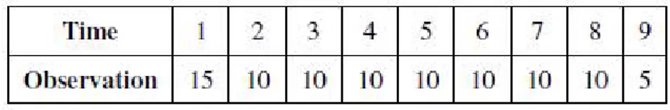
An artificial data set is used for the problem of detecting changes in the mean of a short-run process. Since the posterior distribution of the mean is found in the form of 3mixture model, then the size of is taken as 9 in the application
for getting rid of complexity. The artificial data is given in Table 1.
Table 1. An artificial data set
The prior distribution of process mean () at starting point is defined as 0 ∼
(10 4). Where initial mean of at the 0stage is = 10 and initial variance
of is 2
0 = 4. The likelihood function of the observations is considered as
∼ ( 2). Then the random walk model for the application is stated
as follows: −1 ∼ ⎧ ⎨ ⎩ (−1 2) 1= 08 (−1+ 1 2) 2= 01 (−1− 2 2) 3= 01
The size of a jump in positive direction is taken as 1= 3 and size of a jump
in negative direction is taken as 2= 2 here. Finally, the lower and the upper
threshold values are taken as Tlower = 8 and Tupp er = 13 respectively. An
algorithm designed in Matlab 7.1 which is an extended version of Tsiamyrtzis and Hawkins’s (2005), is used to apply the model to the artificial data. The posterior estimates of the means and posterior probabilities are obtained and presented in the following table.
Table 2. Posterior mean and probability predictions
It is seen that the posterior probabilities which represent the (Tlower
Tupp er) are close to 1 for the 2 to 8 observations. It means there is no
change in the process mean. But it is not valid for the first and the last values of the application. According to posterior probabilities which are close to zero, the jumps in data indicate the real changes in the process mean.
4. Conclusion and Suggestions
In the study, a Bayesian framework is proposed for detecting the change in the unknown mean for a short run process. Since the dynamic structure of
is defined with a random walk containing jumps in both directions at time , the prior and posterior distributions of are found to be in a form of 3 normal
mixture model. Existence of the three possible changes at each time point emphasizes that the number of components in the posterior distribution will increase exponentially with . Therefore, this model is applicable for only short run processes. The process mean has no change when the point estimate of the unknown mean lies within the upper and lower thresholds and the posterior probability is close to 1. In case of violation, the process mean is assumed to have a change in either positive or negative direction. Such change should be checked carefully and necessary interventions should be applied for the real life process control problem.
References
1. Kalman, R. E., A new approach to linear filtering and prediction problems, Journal of Basic Engineering, 82, 35-45, 1960.
2. Montgomery, D. C., Introduction to Statistical Quality Control, 2001.
3. Tsiamyrtzis, P. and Hawkins, D. M., A Bayesian scheme to detect changes in the mean of a short run process, Technometrics, 47, 446-456, 2005.
4. Tsiamyrtzis, P. and Hawkins, D. M., A Bayesian Approach to Statistical Process Control, in Bayesian Process Monitoring, Control and Optimization edited by Colosimo, B.M. and Castillo, E.D., 2007.