An empirical investigation of factors affecting the trade balance of G-20 countries

(1)

International Journal of Economic Perspectives ISSN 1307-1637 © International Economic Society

http://www.econ-society.org

49 An Empirical Investigation of Factors Affecting the Trade Balance

of G-20 Countries

Cüneyt KILIÇ

Canakkale Onsekiz Mart University, Canakkale, Turkey. E-mail:

ckilic2006@hotmail.com.

Feyza BALAN*

Canakkale Onsekiz Mart University, Canakkale, Turkey. E-mail:

feyzarica@gmail.com.

Ünzüle KURT

Ardahan University, Ardahan, Turkey. E-mail: unzulekurt17@gmail.com.

ABSTRACT

During the last twenty years, economic literature has drawn attention to an encouraging role of efficient institutional implements on economic growth. Also, the world oil prices and real exchange rates inevitably are several important variables affecting many macroeconomic parameters of both developed and developing nations on their process of economic growth/development. This paper investigates the effects of institutional quality and of the world oil prices and real effective exchange rates on the trade balance in G-20 countries over the period 1996-2012. Using a static panel data approach, the results of this study demonstrate that the world oil prices, real effective exchange rates and institutional quality are crucial factors on trade balance for G-20 countries. This study also considers the effect of the 2008 Global Economic Crisis and confirms the negative effect of the 2008 crisis on trade balance for G-20 countries.

JEL Classification: C33; 043; F13; F31; Q41.

Keywords: Panel Data Analysis; Institutions; Trade Deficit; Real Effective Exchange Rates; Oil Prices.

*Corresponding author.

1. INTRODUCTION

The term “globalization” has recently been the subject of attention in both academic and policy environment by most economists and policymakers. The process of economic globalization encompasses to increasing integration of economies around the world, particularly through the movements of goods, services, and capital across borders. As economies have become more open to international trade, the transmission of economic fluctuations through trade and financial flows has assumed increased importance. With increasing trade in economies, the trade deficit has been one of the most important issues. Thus, policymakers pay importance the relationship between the exchange rate and the trade balance. In particular, policymakers are concerned about this relationship because exchange rate fluctuations are likely to change the demands for exports and imports thus, affecting the trade balance, gross domestic product, and eventually economic growth.

When investigated the literature subjected to this relationship, we see that there is a popular belief in the international economics literature that the relationship between the exchange rate and the trade balance differs between the short-run and long-run. In particular, it is widely believed that the immediate effect of

devaluation/depreciation of a country's currencyis to lower the trade balance, but this is reversed in the long-run. In other words, following currency depreciation, the trade balance is expected to deteriorate in the short-run before it improves in the long-run, thus; producing a tilted J shape. In the part the literature review of this study, the studies analyzing this relationship will be referred.

In this study investigating the factors of G-20 countries’ trade balance, another independent variable is the world oil price. The effect of oil price shocks on global economy has been a great concern since 1970s and has

(2)

50

triggered a great deal of research investigating macroeconomic consequences of oil price fluctuations. The oil price fluctuations in the trade balance have important place in achieving. The last 40 years in response to the rise in oil prices worldwide economic recession have been observed. Oil prices affect real economic activity mechanism by means of supply and demand channels. The first study investigating the relationship between oil prices and the trade balance belongs to Agmon and Laffer (1978). Agmon and Laffer (1978) found that the trade balance of industrialized countries deteriorated markedly immediately following an oil price increase in the initial period, but after that initial deterioration these trade balances improved again.

In this study besides real effective exchange rate and the world oil prices, we use institutional factors as one of the independent variables with reference to research evidence on the pivotal role of institutions in economic and social activities. Indeed institutions are hidden factors within the economic system, and it is hard to find one proxy which would suitably represent the quality of the countries’ institutions. In this study, we use the World Bank’s World Governance Indicators produced by Kaufmann, Kraay, Mastruzzi. Kaufmann, Kraay and Mastruzzi (2010) construct the governance with six dimensions: voice and accountability, political stability, government effectiveness, regulatory quality, rule of law, control of corruption. We use the summation of these six dimensions as a proxy variable of institutional quality.

The remainder of this paper is organized as follows. Section 2 outlines the previous literature, Section 3 discusses the data set and the methodology and presents the empirical findings and Section 4 concludes the paper.

2. LITERATURE REVIEW

Bahmani-Oskooee (1985) examined whether the J curve phenomenon is valid for a sample of developing countries over the period 1973-1980. The empirical results showed that the J curve phenomenon is exactly for the trade balance of the selected countries except for Thailand. Another study, Nusair (2013) tested the J-curve phenomenon for seventeen transition economies using montly data over the period 1991-2012. Using the conditional ARDL bounds testing approach, Nusair (2013) suggest that the J-curve phenomenon is supported for only three countries from seven countries.

Arize (1994) investigated the long-run relationship between the real effective exchange rate and the trade balance in nine Asian economies over the period 1973Q1 and 1991Q1. The findings showed that there exists a significantly positive link between the two variables in Asia.

Using the co-integration technique in order to assess the long-run relation between the trade balance and the real effective exchange rate, Bahmani-Oskooee and Alse (1994) find that the trade balance and the real effective exchange rate are cointegrated for six countries from twenty countries. For most countries, the two variables were found to be not cointegrated, indicating that devaluations cannot have any long-run effects on the trade balance in the period 1971Q1-1990Q4. This result was interpreted as not being supportive finding to the J-curve phenomenon by the authors. Similarly, In and Menon (1996) investigated whether the real exchange rate and the terms of trade are cointegrated for seven major OECD countries. They find that the two variables are cointegrated and exchange rate changes Granger cause changes in the terms of trade for five of seven OECD countries.

Dollar and Kraay (2003) investigated the partial effects of institutions and trade on economic growth and find that rapid growth, high levels of trade, and good institutions go together. They conclude the paper that both trade and institutions are important in understanding cross-country differences in growth rates in the very long-run. Baliamoune-Lutz and Ndikumana (2007) investigated whether trade openness contributes to higher income and whether institutions affect the growth of trade for 39 African countries covering the period 1975-2001 by using Arellano-Bond panel estimation techniques. The empirical results suggest that institutions have an important influence on the effectiveness of trade policy and institutions have a positive impact on growth.

Shao (2008) studied the economic factors influencing the bilateral trade balance between Japan and the US. in the period 1980-2006. The results indicate that Japan’s trade balance has a significantly positive relationship with the exchange rate in short run. Furthermore, the results show that the US. GDP has a larger than Japan’s GDP permanently positive relation on Japan’s trade balance.

(3)

51

Faria et al. (2009) developed a theoretical model that explains the positive relationship between Chinese exports and the oil price. The model shows that Chinese growth can lead to an increase in oil prices that has a stronger impact on its export competitors.

Hassan and Zaman (2012) examined the link among trade balance, oil price, and exchange rate shocks in Pakistan over a period of 1975-2010. Using ARDL approach, the results of the study indicate that there is a significantly negative relation among oil prices, exchange rate and trade balance of Pakistan. The authors concluded the paper that oil prices and exchange rate induces trade imbalance in Pakistan.

3. DATA, MODEL AND ECONOMETRIC METHODOLOGY

3.1. Data and Model

This study uses annual data from 1996 to 2012 for G-20 countries in order to empirically investigate the factors affecting trade balance of G-20 countries1. This empirical study is based on data balance of trade, is the difference between the monetary values of exports and imports an economy, the world oil prices, real effective exchange rates and institutional quality reflecting six dimensions of governance. Balance of trade data and the world oil prices data have been obtained from the World Bank’s World Development Indicators, real effective exchange rate index have been obtained from Bank for International Settlements, and institutional quality data have been obtained from the World Bank’s Worldwide Governance Indicators produced by Kaufmann, Kraay, Mastruzzi (2010). In order to carry out the paper E views 7.0, Gauss 6.0 are used.

Econometric Model

Following the literature our study applies a static panel data (Fixed Effects) analysis. The fixed effect version of the model, which will be estimated is specified as follows:

1.OIL_W 1 2.REXCH 3.INST 4. .

it i i it i it i it it

BOT = +c γ +β −+β +β +β CRISIS +ηt+ε (1)

where, c is constant term, γ represents the cross-section or country fixed effect, i BOTitis balance of trade of

country i in year t, OIL W_ itis the world oil price in year t, REXCHitis the real effective exchange rate index of

country i in year t, INST_it is institutional quality of country i in year t, CRISIS is a dummy variable that captures the existence of the financial crisis of 2008, η captures a common deterministic trend. .t

3.2. Econometric Methods and Findings

The first issue is to test whether or not slope coefficients are homogenous in our empirical model. It does not allow us to capture heterogeneity due to country specific characteristics, if the slope homogeneity is assumed without any empirical evidences (Breitung 2005). An homogenous panel data model (or pooled model) is a model in which all coefficients are common while an heterogenous panel data model is defined as a model in which all parameters (constant and slope coefficient) vary across individuals (Hurlin, 2010). The estimation methods differentiate in accordance with the selection of a homogenous panel or heterogeneous panel data. This study applies Pesaran and Yamagata’s (2008) homogeneity test.

3.2.1. Pesaran and Yamagata (2008)’s Homogeneity Test

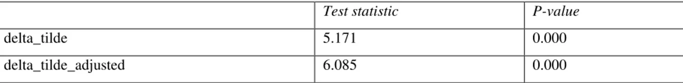
Pesaran and Yamagata (2008) proposed delta_tilde test for testing slope homogeneity in large panels. Under the null hypothesis of slope homogeneity with the condition of (N,T) → ∞, so long as N_T → ∞ and the error terms are normally distributed, the delta_tilde statistic has an asymptotic standard normal distribution. The small sample properties of the statistic can be improved under the normally distributed errors with bias adjusted statistic (delta_tilde_adjusted) suggested by Pesaran and Yamagata (2008). Thus, we rely on the result regarding delta_tilde_adjusted statistic. Results for the homogeneity test of Pesaran and Yamagata (2008) are illustrated in Table 1. Since the p-value of delta_tilde_adjusted is smaller than 0.05 significance level, we can

1

Argentina, Australia, Brazil, Canada, China, France, Germany, India, Indonesia, Italy, Japan, Republic of Korea, Mexico, Russia, Saudi Arabia, South Africa, Turkey, the United Kingdom, the United States and the European Union.

(4)

52

reject that slope coefficients don’t vary across individuals. Consequently, it is clear that the null of hypothesis Pesaran and Yamagata (2008)’s homogeneous test is rejected at 95%.

Table 1. Pesaran and Yamagata (2008)’s Homogeneity Test

Test statistic P-value

delta_tilde 5.171 0.000

delta_tilde_adjusted 6.085 0.000

3.2.2. Unit Root Characteristics

The second issue in our analysis is to examine stationary properties of the dataset. Firstly, we test the existence of cross-sectional dependence across countries. Pesaran (2006) showed that ignoring cross-section dependency leads to substantial bias and size distortions in estimation of the relationship between two variables. In this study, we apply the cross-section dependence LM (CDLM) tests developed by Pesaran (2004) to verify the consideration of cross-section dependence in investigating the factors affecting G-20 countries’ trade balance. Three LM tests have been applied to check cross sectional dependency. One of them, CDLM1 was developed by Breusch Pagan (1980). Other LM tests are CDLM2 and CDLM tests that were developed by Pesaran (2004). CDLM1 test is useful when N is fixed and T goes to infinity. CDLM is better to use when N is larger and T is smaller. CDLM2 test is useful when T and N are larger enough (Guloglu and Ivrendi, 2008: 4).

In this study, we carried out two different tests that are suitable for this type of analysis to investigate the existence of cross-sectional dependence and illustrated the empirical results in Table 2. It is clear that null of no cross-sectional dependence across the members of panel is not strongly rejected at the conventional levels of significance. The cross-sectional independence across the G-20 countries indicates that a shock to the trade balance, real exchange rate, and institutional quality in a country is not likely to affect other G-20 countries. Table 2. Cross Section Dependence Test Results

Constant+Trend

BOT REXCH INST

Statistic p-value Statistic p-value Statistic p-value

lm

CD

(Pesaran,2004) -0.313 0.377 -0.078 0.469 -1.338 0.090 adj

LM

(PUY,2008) -1.837 0.967 -1.372 0.915 -3.178 0.999

After analyzing cross-section dependency, we control whether there exists unit root in the series in order to get unbiased estimations. Several different panel unit root tests are available. Many recent studies rely on panel unit root tests in order to increase the statistical power of their empirical findings. In this respect, we have used the approaches of Im et al. (2003, henceforth IPS), Maddala and Wu (1999, henceforth MW), Choi (2001) as the panel unit root tests. The IPS test allows for residual serial correlation and heterogeneity of the dynamics and error variances across units. The IPS (2003) testing procedure is written in Equation (2) as follows:

, , 1 , 1 . . . k i t i i i t i t j i t j it j Y µ ρ Y ₋ δ t φ α Y ₋ ε = ∆ = + + + +

∑

∆ + (2)

Testing for unit root in the panel is based on the Augmented Dickey Fuller (ADF) statistics averaged across groups. Hypothesis of IPS may be specified as follows:

0: i 0

H ρ = HA:ρip0for all i

The alternative hypothesis allows that for some (but not all) of individuals series to have unit roots. IPS compute separate unit root tests for the N cross-section units. IPS define their t-bar statistics as a simple average of the individual ADF statistics, ti, for the null as:

1 / N i i t t N = =

∑

(5)

53

It is assumed that ti are i.i.d and have finite mean and variance and E(ti), Var(ti) is computed using Monte-Carlo

simulation technique. Other test MW is based on a combination of the p-values of the test statistics for a unit root in each cross-sectional unit. The null and alternative hypotheses are the same as those of the IPS test. Unlike the IPS test, the procedure advocated by MW does not require a balanced panel and it is non-parametric (Kónya 2001). MW define λ test statistic as follows:

2 2 1 2 ln n i n i p λ χ = = −

∑

where π denotes the p-value from the ADF test on the ii

th

time series. MW and Choi approaches have the same framework. Choi (2001) proposes a Z test and shows that when N also tends to infinity, Z may be standardized as follows (Erlat 2009): i i 1 1 2ln 2 2 N Z p N = =

_∑

− −

where Z have an asymptotic N (0,1) distribution.

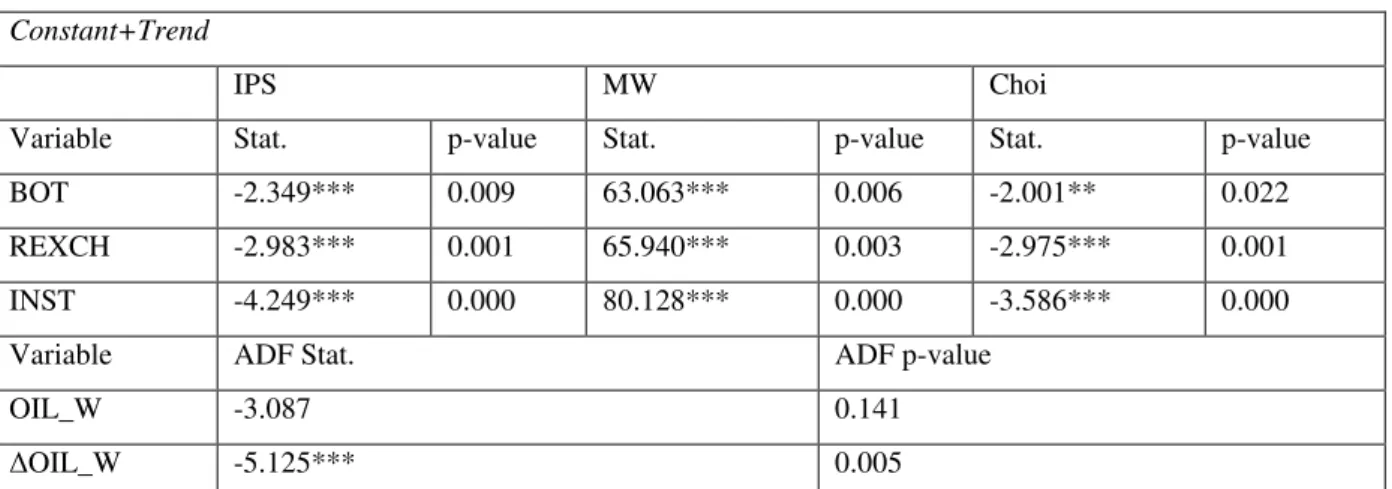
The results of unit root tests for the series are illustrated in Table 3. Results in Table 3 show that the series, except for OIL_W, are I(0). The ADF test statistic for the first-difference of OIL_W strongly rejects the null hypothesis, which implies that the variable is stationary in the first-difference form. Thus, we use the dataset contains the stationary series, which are BOT, REXCH, INST, ΔOIL_W.

Table 3. Results for Unit Root Tests

Constant+Trend

IPS MW Choi

Variable Stat. p-value Stat. p-value Stat. p-value

BOT -2.349*** 0.009 63.063*** 0.006 -2.001** 0.022

REXCH -2.983*** 0.001 65.940*** 0.003 -2.975*** 0.001

INST -4.249*** 0.000 80.128*** 0.000 -3.586*** 0.000

Variable ADF Stat. ADF p-value

OIL_W -3.087 0.141

ΔOIL_W -5.125*** 0.005

Notes: Δ is the first difference operator. The maximum lag lengths were set to 3 and Schwarz Bayesian Criterion was used to determine the optimal lag length. ***,** denote the rejection of the null at the 1% and 5% levels respectively.

3.2.3. Static Panel Data Analysis

We use a specific country group (G-20 countries) in the study so fixed effect panel data analysis is useful (Baltagi, 2008: 14). Panel data may have group effects, time effects, or both. These effects are either fixed effect or random effect. A fixed effect model assumes differences in intercepts across groups or time periods. Fixed effects model explores the relationship between the predictor and outcome variables within an entity. This entity may be households, countries, firms. The model assumes all other time invariant variables across entities that can influence the predictor variables to be constant.

it i t it

u =µ +λ +v i= 1,…,N t=1,…,T

where µi denotes the unobservable individual effect, λtdenotes the unobservable time effect, and vit is the

stochastic disturbance term. λ is individual-invariant and it accounts for any time-specific effect that is not t

(6)

54

If the µ and i λt are assumed to be fixed parameters to be estimated and vit IID (0,

2

v

σ ), then the above regression represents a two-way fixed effects error component model (Baltagi, 2005).

Fixed effects model can be formulated as:

' .

it it i it

y =x β α+ +ε (3)

where α denotes all the observable effects and it is group-specific constant term in the regression model. i α i

equals ' .

i

z α in the regression (3). If z_i is unobserved, but correlated with

x

_it, then the coefficient of β is biased and inconsistent under assumptions of E u( it)=0;

2 2

( it)

E u =σ all i; E u u( it. jt s−)=0 for s≠0 and i≠ j

0 .

it it i t it

y =α +X β α+ +γ +ε (4)

Equation (4) can be formulated as a two-way fixed effects model controlling for unmeasured time-invariant differences between units and unit-invariant differences between time periods. α denotes individual-specific i

effects and γ_t denotes period-specific effects.

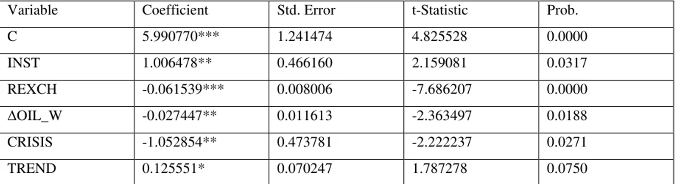
Table 4 reports the panel estimation results using the trade balance as the dependent variable as in Equation (1), controlling for the existence of the 2008 financial crisis, in which case the dummy variable CRISIS assumes the value of one (zero otherwise). From Table 4, we can see that increases in real effective exchange rate and the world oil prices have a significantly negative impact on the G-20 countries’ trade balance. Thus, we can say that the J-curve phenomenon is not valid in the short-run for G-20 countries. In addition, institutional quality, representing the summation of the indexes of voice and accountability, political stability, government effectiveness, regulatory quality, rule of law, control corruption improves G-20 countries’ trade balance while the financial crisis of 2008 deteriorates G-20 countries’ trade balance. Consequently, we can say that institutional quality, real effective exchange rate, and the world oil prices are important determinants of G-20 countries’ trade balance.

Table 4. Results for Panel Least Squares Method

White Cross-Section Standard Errors and Covariance (d.f.corrected)

Variable Coefficient Std. Error t-Statistic Prob.

C 5.990770*** 1.241474 4.825528 0.0000 INST 1.006478** 0.466160 2.159081 0.0317 REXCH -0.061539*** 0.008006 -7.686207 0.0000 ΔOIL_W -0.027447** 0.011613 -2.363497 0.0188 CRISIS -1.052854** 0.473781 -2.222237 0.0271 TREND 0.125551* 0.070247 1.787278 0.0750

Note: Δ is first difference operator and ***,**,* indicate the statistical significance at 1%, 5% and 10% levels respectively.

4. CONCLUSIONS

This paper investigates empirically the key factors influencing the trade balance using data for G-20 countries for the period 1996-2012. In particular, we analyze the impact of the real effective exchange rate index, the world oil price, institutional quality index, the financial crisis of 2008 on the trade balance for G-20 countries with panel data estimation technique.

Estimation using panel data has advantages over purely cross-sectional estimation as it would take into account, besides considering the cross-country relationship between the variables; how institutional quality, real effective exchange rate over time within a country may have an effect on the country’s trade balance. Moreover, working with panel data model helps to overcome unobserved country-specific effects and thereby reduce biases in the estimated coefficients.

(7)

55

The empirical results based on the fixed effects model show that the real effective exchange rate index, the world oil price, the institutional quality index are important factors in explaining G-20 countries’ trade balance. Especially, our findings that depreciation has no short-run positive effect on the trade balance imply that the selected economies may not use exchange rate policy to increase exports and promote economic growth in the long-run.

The empirical evidence also showed by the regression is in line with the hypothesis that institutional quality has a significant positive impact on trade balance for G-20 countries. Thus, we can say that countries with better institutions also tend to trade more and the institutional quality needs to be improved in case of the participation of the countries’ citizens in selecting their government and the quality of regulation.

REFERENCES

Agmon, T. and Laffer, A. B. (1978). Trade, Payments and Ad-justment: The Case of Oil Price Rise, Kyklos, 31, 68–85.

Arize, A. C. (1994). Cointegration Test of a Long Run Relation Between the Real Effective Exchange Rate and the Trade Balance, ,International Economic Journal, 8(3), 1–9.

Bahmani-Oskooee, M. (1985). Devaluation and the J-Curve: Some Evidence from LDC’s, The Review of

Economics and Statistics, Vol.67, No.3, 500–504.

Bahmani-Oskooee, M. and Alse, J. (1994). Short-run versus long-run effects of devaluation: Error-correction Modeling and Cointegration, Eastern Economic Journal, Bloomsburg: Fall , Vol.20 (4), 453-464.

Baliamoune-Lutz, M. and Ndikumana, L. (2007). The Growth Effects of Openness to Trade and the Role of Institutions: New Evidence from African Countries. University of Massachusetts Economics Department

Working Paper Series, Paper 38, 1-28.

Baltagi, B. (2005). Econometric Analysis of Panel Data, Third Edition, Chichester: John Wiley & Sons, Ltd. Baltagi, Badi. H. (2008). Econometric Analysis of Panel Data (4th Ed.). John Wiley & Sons, Ltd.

Bank for International Settlements (BIS). http://www.bis.org/statistics/eer/.

Breitung, J. (2005). A Parametric Approach to the Estimation of Cointegration Vectors in Panel Data,

Econometric Reviews, 24, 151–173.

Breusch, T. S. and Pagan, A. R. (1980). The Lagrange Multiplier Test And Its Applications To Model Specification In Econometrics, Review of Economic Studies, Blackwell Publishing, Vol. 47 (1), 239–253. Choi, I. (2001). Unit Root Tests for Panel Data, Journal of International Money and Finance, 20, 249–272. Dollar, D. and Kraay A. (2003). Institutions, trade, and growth, Journal of Monetary Economics, Vol. 50(1), 133-162.

Erlat, H. (2009). Persistence in Turkish Real Exchange Rates: Panel Approaches, FIW-Working PAPER, No:29, 1-32.

Faria, J.R., Mollick, A.V., Albuquerque P.H. and León-Ledesma, M.A. (2009). The Effect of Oil Price on China's Exports, China Economic Review, 20, 793–805.

Guloglu, B. and Ivrendi M. (2008). Output fluctuations: Transitory or permanent? The case of Latin America,

Applied Economics Letters, 1-6.

Hassan, A.S. and Zaman, K. (2012). Effect of Oil Prices on Trade Balance: New insights into the Cointegration Relationship from Pakistan, Economic Modelling, 29, 2125–2143.

(8)

56

Hurlin, C. (2010). What would Nelson and Plosser Find Had They Used Panel Unit Root Tests?, Applied

Economics, 42(12), 1515-1531.

Im, K.S., Pesaran, M. H. and Shin, Y. (2003). Testing for Unit Roots in Heterogeneous Panels, Journal of

Econometrics, 115, 53-74.

In, F. and Menon, J. (1996). The Long-run Relationship between the real Exchange rate and terms of trade in OECD countries, Applied Economics, 28,1075–1080.

Kaufmann, D. Aart K. and Massimo M. (2010). The Worldwide Governance Indicators: A Summary of Methodology, Data and Analytical Issues, World Bank Policy Research Working Paper, No.5430, 1-29.

Kónya, L. (2001). Panel Data Unit Root Tests with an Application, Discussion Paper, School of Applied

Economics, Victoria University, Melbourne, Australia.

Maddala, G. and Wu, S. A. (1999). Comparative Study of Unit Root Tests and a New Simple Test, Oxford

Bulletin of Economics and Statistics, 61, 631–652.

Nusair, S. A. (2013). The J-curve in transition economies: An application of the ARDL model, Academic and

Business Research Institute International Conference, New Orleans: Academic and Business Research Institute, 1–31.

Pesaran, M. H. (2004). General diagnostic tests for cross section dependence in panels, University of Cambridge,

Working Paper, No.0435, 1-39.

Pesaran, M. H. (2006). Estimation and inference in large heterogeneous panels with multifactor error structure,

Econometrica, 74, 967-1012.

Pesaran, M. H. and Takashi Y. (2008). Testing slope homogeneity in large panels, Journal of Econometrics, 142, 50–93.

Shao, Z. (2008). Exchange Rate Changes and Trade Balance: An Empirical Study of the Case of Japan, Online available at: http://ink.library.smu.edu.sg/etd_coll/ 15 (2008) (accessed on 2nd February, 2012).

U.S. Energy Information Administration’s International Energy Statistics, http://www.eia.gov. World Bank, http://data.worldbank.org/indicator.

(9)

An empirical investigation of factors affecting the trade balance of G-20 countries

49