Variation of air concentration in ski jump jets

Adıyaman Üniversitesi

Mühendislik Bilimleri Dergisi

13 (2020) 75-88

VARIATION OF AIR CONCENTRATION IN SKI JUMP JETS

1_{Şırnak Üniversitesi, Mühendislik Fakültesi, İnşaat Mühendisliği Bölümü, Şırnak, 73000, Türkiye} Geliş tarihi: 18.06.2020 Kabul tarihi: 03.09.2020

ABSTRACT

Scour is a significant problem for the stability and safety of a dam. Water jet issued from flip bucket of a dam creates an air-water mixture and finally plunges at the downstream of a dam. Depending on the discharge, total head, thickness of the water body, aeration conditions and geometrical features of the flip bucket, the jet is dispersed in air. It is obvious that air concentration is inversely proportional with the dynamic pressures at impingement area of the water jet coming from the flip bucket of spillway of a dam. Impact of the ski jump jet at the impingement point may be reduced depending on the air concentration of the jet. In this study, experimental and numerical assessments are performed to analyze the distribution of the air into the ski jump jet depending on the dynamic pressures at the impingement point. The impact of the ski jump jet is analyzed and air percentages are defined into the jet according to dynamic pressure measurements using pressure transmitters at the impingement area. By doing so, aeration characteristics and impact values of water jets are revealed to generate reliable scour estimations.

Keywords: Spillway, air concentration, ski jump jets, dynamic pressure distribution, jet dispersion, numerical

solution

DOLUSAVAKLARDA SIÇRATMA EŞİĞİNDEN ÇIKAN SU JETİ HAVA

KONSANTRASYONUNUN DEĞİŞİMİ

ÖZET

Baraj stabilitesi ve güvenliği için baraj mansabındaki oyulma her zaman önemli bir tehdit olmuştur. Sıçratma eşiğinden çıkan su jeti hava-su karışımı oluşturur ve sonrasında barajın mansap tarafına düşer. Su jeti debi, toplam enerji yüksekliği, su jetinin büyüklüğü, havalanma koşulları ve sıçratma eşiğinin geometrik özellikleri gibi parametrelere bağlı olarak havada yayılır. Su jetinin düştüğü noktada oluşan dinamik basınç dağılımı jetin içerisinde bulunan hava konsatrasyonu ile ters orantılı olarak değişir. Buna göre, su jetinin düştüğü noktadaki oyulma büyüklüğü jetin hava konsantrasyonunun artırılması ile düşebilir. Bu çalışmada, su jeti içerisindeki hava konsantrasyonu, nehir yatağında oluşan dinamik basınçların deneysel ve nümerik değerlendirmesi yapılarak incelenmiştir. Su jetinin düşme noktasındaki etkisi basınç sensörleri ile belirlenen dinamik basınçlar ile ölçülmüş ve hava konsantrasyonu yüzdeleri buna görebelirlenmiştir. Böylece, güvenilir bir su jeti hava konsantrasyonu analizi bu çalışma ile sağlanmıştır.

Anahtar Kelimeler: Dolusavak, hava konsantrasyonu, su jeti, dinamik basınç dağılımı, jet yayılımı, nümerik

çözümleme

1. Introduction

Numerous experimental and numerical investigations in air-water mixture issued from a spillway of a dam were carried out during the last century[1-5]. These investigations show that air concentration into the water jet mostly depends on the geometrical features of the flip bucket and boundary conditions. Flip bucket at the end of a spillway of a dam assessed to be a good application to dissipate the energy of the water jet with high velocities [6-8].

Flip buckets can be designed in various shapes and scales according to geological and economic circumstances involving relative curvature, deflection angles, take-off angles and special components. However, It is stated that, there is only a few guidelines are available to standardize the flip buckets [9]. Heller et al. [10] conducted experiments to investigate the two-dimensional jet trajectories. Bucket angle, trajectory angle, jet trajectories with different air concentration ratios and pressure distributions on the flip bucket were also examined for minimum model approach flow depth of around 40 mm. Steiner R., Hager W.H., and Minor H.E. [11] decided to investigate the effects of the triangular-shaped flip bucket placed at the take-off of ski jump rather than the general form of the circular-shaped bucket. They revealed that, pressure on the flip bucket depends on the approach flow Froude number and the deflector angle of the bucket and energy dissipation of the water jet depends on the deflector angle of the flip bucket and the drop height of the bucket take-off to the channel. Limits of the Froude number are determined according to the model to prevent choking of the spillway bucket[11].

Chanson [12] studied some experiments on naturally occurred air entrainment into turbulent water jets and compared the results with two-dimensional jet calculations using empirical equations for jet velocities between 4.5 and 36.5 m/s Schmocker et al. [13] mentioned that, water jet dispersion into the air and air concentration into the jet greatly depend on the jet velocity, height of the spillway and geometrical structure of the bucket lip located at the end of the spillway. Kawakami [14] showed that aeration of the water jets from flip buckets reduce the trajectory length based on the field data. Kawakami [14] developed some empirical equations and an aeration constant to calculate the jet length with air entrainment from the flip bucket lip to the impingement point of the jet. In this study, air concentration of the ski jump jet at impingement area is studied experimentally. Measured, calculated and simulated trajectory lengths are compared to validate the reliability of the method used in the study. Reliable estimation of air concentration in water jet is extremely significant to prevent adverse effects of scour at the downstream of a dam.

The study differs from the previous researches with its accurate dynamic pressure evaluations and air concentration determination method. Hereby, it may shed light on a better scour estimation at the downstream of a dam. Necessary precautions might be taken in advance with refering the results of this study in order not to experience a stability problem generated by an extreme scour in the river bed.

2. Experimental Facility

Experiments were conducted for 6 different discharges starting from 0.07 m3_{/s to 0.22 m}3_{/s by}

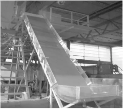
adding 0.03 m3_{/s on the previous test discharge. 1:25 scaled hydraulic model of Laleli Dam and HEPP}

[15] was used for experimental investigations in Hydromechanics laboratory of Middle East Technical University (METU) (Figure 1).

Height of the ogee crested weir of the spillway from the lip of the bucket is 3.8 m. Model spillway has 0.8 m width and the angle of the spillway is 550_{. Cross-sectional view of the spillway}

Figure 1 Hydraulic Model of the Study

Figure 2 Cross-sectional view of the spillway

Jet velocities, trajectory lengths and jet dispersions at the impingement point were measured from the experimental set up for every single discharge. Trajectory lengths were calculated by using Kawakami’s formula to determine the installment location of the pressure transmitters.

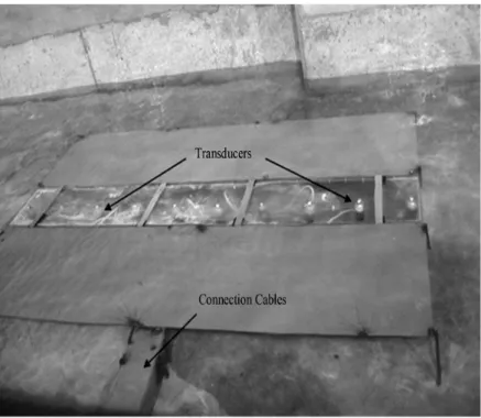
10 pressure transmitters of type 501 produced by Huba Control were positioned at the impingement area of the water jet coming from the flip bucket lip. The positions of the transmitters were arranged depending of the aerated trajectory length calculations using Kawakami’s formula (Figure 3).

z

=1.2 m

α

=55

Figure 3Position of the pressure transmitters in the impingement area

Metal plates were fixed at the both sides of the pressure transmitters to compensate the elevation difference adjacent to the transmitter box. Adjusted and amplified sensor signals were recorded and converted into digital data by using DAQ software [16].

Dynamic pressures were recorded for a period of 180 seconds and digitized at 40 Hz frequency for every test case. These pressure data were evaluated to determine dynamic pressure variations into the impingement area. Since the dynamic pressure and the air concentration can be assumed inversely proportional, the air concentration of the water jet can be determined depending on the pressure variations obtained from the pressure transmitters.

3. Methodology

3.1. Trajectory Length Determinations

3.1.1. Measured and Calculated Trajectory Lengths

Positioning of the pressure transmitters is one of the most significant steps to perform dynamic pressure measurements for determining the air concentration of water jet at the impingement area. Therefore, trajectory lengths with air entrainment for the selected discharges should be precisely defined. Trajectory lengths were calculated for every single test case using the jet velocities measured on the flip bucket lip. Positions of the pressure transmitters were determined according to the calculated trajectory lengths using Kawakami’s equations [14]. To check the correctness of the calculations, experiments were conducted for the selected discharges and trajectory lengths were also measured from the experimental facility. Additionally, Flow 3D simulations were conducted to determine aerated trajectory lengths. All these measured, calculated and computed trajectory lengths were compared to generate a reliable estimation of air concentration in ski jump jets.

Kawakami [14] proposed the following equations to determine the trajectory lengths with air entrainment.

𝐿𝐿 = �_{𝑔𝑔𝑘𝑘}1₂� 𝑙𝑙𝑙𝑙�1 + 2𝑘𝑘𝑘𝑘𝑉𝑉𝑗𝑗𝑐𝑐𝑐𝑐𝑐𝑐 𝑘𝑘𝑗𝑗� (1)

where

𝑘𝑘 = 𝑡𝑡𝑡𝑡𝑙𝑙−1_{�𝑘𝑘𝑉𝑉}

𝑗𝑗𝑐𝑐𝑠𝑠𝑙𝑙 𝑘𝑘𝑗𝑗� (2)

and L is trajectory length with air entrainment, k is Kawakami’s aeration constant, αj is the water jet angle and Vj is the jet velocity at the lip of the flip bucket.

Figure 4 was also prepared by Kawakami [14] to present the relationship between the aeration constant and trajectory lengths vs prototype jet velocities. In the figure, αj is the water jet angle at the bucket lip, Lt is the trajectory lengths obtained from projectile motion theory. In projectile motion theory, the motion occurs in a frictionless domain. So, Lt can be denoted as trajectory length without air entrainment. The parameters shown in Figure 4 are applicable to all types of design for the given jet velocity intervals.

Since Kawakami’s investigations were based on the field data, air concentration constant was defined for prototype velocities. Therefore, Froude Similarity law must be used to calculate equivalent prototype jet velocities. By doing so, the air concentration constant can be obtained from Figure 4.

Figure 4 Relationship between the aeration constant and trajectory lengths vs prototype jet velocities

proposed by Kawakami [14] 3.1.2. Simulated Trajectory Lengths

Characteristics of flow in experimental studies can also be determined using numerical model applications generally named as Computational fluid dynamics (CFD). A model is generated into mesh format to investigate the conditions of flow and flow characteristics using computer programs (i.e. Fluent, Flow 3D). Principal flow equations like Navier-Stokes and continuity are solved for every single mesh of the model. However, if the numerical model is not generated appropriately, the

L Lt αj Vj(m/s) 0.03 0.01 0.02 0_{10 20 30 40} k Vj(m/s) 0.75 0.25 0.50 0_{10 20 30 40} L Lt 1.00 z

solutions obtained by CFD might be specious. To refrain from these kinds of misleading outcomes, numerical solutions should be verified with experimental studies.

Commercial CFD code Flow 3D was used for the numerical solution of the study. Reynolds-Averaged Navier-Stokes (RANS) equations were used for an incompressible, Newtonian fluid in the numerical model. The k-Ɛ model of turbulence was used in the computation of Reynolds stresses and turbulent viscosity [17]. Especially for the flows with high Reynolds numbers, k-Ɛ model can be advantageous [18].

RANS and continuity equations, Eqs. (3) and (4), used for the numerical model are given below. 𝜕𝜕 𝜕𝜕𝜕𝜕𝑖𝑖(𝑢𝑢𝑖𝑖𝐴𝐴𝑖𝑖) = 0 (3) 𝑢𝑢𝑗𝑗𝜕𝜕𝑢𝑢_{𝜕𝜕𝜕𝜕}𝑖𝑖 𝑖𝑖 = − 1 𝜌𝜌 𝜕𝜕𝜕𝜕 𝜕𝜕𝜕𝜕𝑖𝑖+ 𝜗𝜗 𝜕𝜕2_𝑢𝑢 𝑖𝑖 𝜕𝜕𝜕𝜕𝑗𝑗𝜕𝜕𝜕𝜕𝑗𝑗+ 1 𝜌𝜌 𝜕𝜕𝜏𝜏𝑖𝑖𝑗𝑗 𝜕𝜕𝜕𝜕𝑗𝑗 + 𝑓𝑓𝑖𝑖 (4) where xi and xj are Cartesian coordinate components, ui is the velocity component in direction i, Ai is the fractional area in the direction i, ρ is the density, P is the pressure and fi is the body forces and ν is the kinematic viscosity and τij is the Reynolds stress for a turbulence model respectively. In order to reduce the equations for incompressible ones; Aj is taken equal to 1. For k-Ɛ model, Reynolds stress can be found using the following equation, Eq. (5).

𝜏𝜏 𝑖𝑖𝑗𝑗= −𝜌𝜌𝑢𝑢𝑖𝑖`𝑢𝑢𝑗𝑗`= 2𝜌𝜌𝑣𝑣𝑡𝑡𝑆𝑆𝑖𝑖𝑗𝑗−2_{3 𝜌𝜌𝑘𝑘𝛿𝛿}𝑖𝑖𝑗𝑗 (5)

where 𝑢𝑢𝑖𝑖` and 𝑢𝑢𝑗𝑗`are the fluctuating velocity components, vt is the eddy viscosity, Sij is the strain-rate tensor and δij is the kronecker delta. The equations of these parameters, Eqs. (6), (7) and (8), are also defined as follows; 𝑣𝑣𝑡𝑡 = 𝐶𝐶𝜇𝜇𝑘𝑘_𝜀𝜀 (6) 𝑆𝑆𝑖𝑖𝑗𝑗=1_{2 �}𝜕𝜕𝑢𝑢_{𝜕𝜕𝜕𝜕}𝑖𝑖 𝑗𝑗+ 𝜕𝜕𝑢𝑢𝑗𝑗 𝜕𝜕𝜕𝜕𝑖𝑖� (7) 𝛿𝛿𝑖𝑖𝑗𝑗 = �1 𝑠𝑠𝑓𝑓 𝑠𝑠 = 𝑗𝑗_{0 𝑠𝑠𝑓𝑓 𝑠𝑠 ≠ 𝑗𝑗�} (8)

where Cµ is a coefficient and taken as 0.09 for a standard k-Ɛ model [19]. k-Ɛ model is also elaborated in Speziale`s studies [20].

Flow 3D, which is appropriate commercially available CFD software, uses Fractional Area Volume Obstacle Representation (FAVOR), improved Volume Of Fluid technique (VOF) and multi block meshing to increase its capabilities [21]. Since it was not possible to measure the air concentration of the water jet coming from the flip bucket of the hydraulic model, only calculated and simulated trajectory lengths of the jets were compared using experimental setup and FLOW-3D, respectively. Furthermore, two-phase numerical flow analysis was evaluated as useless due not to create a probable comparison between experimental and numerical air concentrations.

AutoCAD, which is commercially available computer aided software, was used to generate a model of the test facility and saved as .stl format to employ in Flow 3D. Free gridding method was used to discretize the flow domain. In this way, the required time for the grid generation and computation can be significantly decrease. Not to cause any misleading on determining the slip effects between the water, boundary of the model and wall shear stresses, mesh sizes were designed as 100

mm in x direction, 20 mm in y direction and 50 mm in z direction, respectively. Initial flow conditions for the reservoir were assumed to be constant for 3000 mm upstream of the spillway crest and were fixed for each test case (Figure 5).

Figure 5 Side view of the numerical model of the experimental test facility

Boundary conditions were described for side walls, top of the spillway and downstream of the model as symmetrical, and for flow inlet as constant water height with specified pressure. Time intervals were defined as depending on Courant–Friedrichs–Lewy (CFL) condition. The numerical model was generated as 3D and computations were done for this model accordingly.

3.2. Determination of Air Concentration

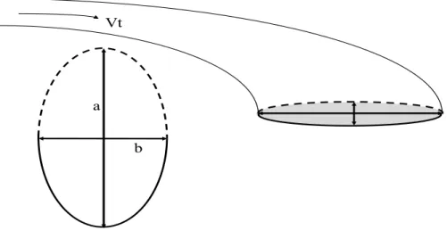
The amount of dispersion of water jet in the air was measured from the photos taken during the experiments. Impingement area of the aerated jet was measured to determine the air-water percentage at the point of impact. This area was assumed to be elliptic (Figure 6) and air-water ratios were found based on mass conservation of the water jet.

Figure 6 Measurement method of impingement area on the water surface

The longitudinal dimension ‘b’ and the lateral dimension ‘a’ were determined for each test case and Vt

a

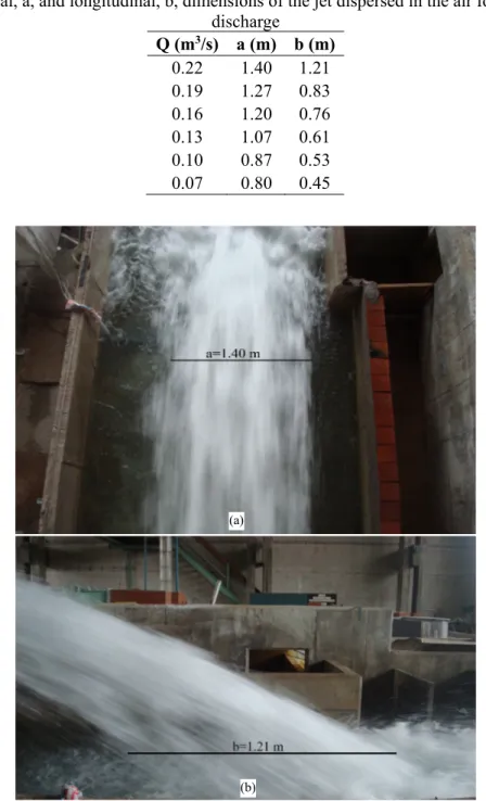
results are summarized in Table 1. The sample photographs indicating the measurement for Q = 0.22 m3_{/s are shown in Figure 7.}

Table 1 Lateral, a, and longitudinal, b, dimensions of the jet dispersed in the air for every single

discharge Q (m3_{/s) a (m) b (m)} 0.22 1.40 1.21 0.19 1.27 0.83 0.16 1.20 0.76 0.13 1.07 0.61 0.10 0.87 0.53 0.07 0.80 0.45

Figure 7 Lateral (a) and longitudinal (b) dimensions of the dispersed jet for Q = 0.22 m3_/s

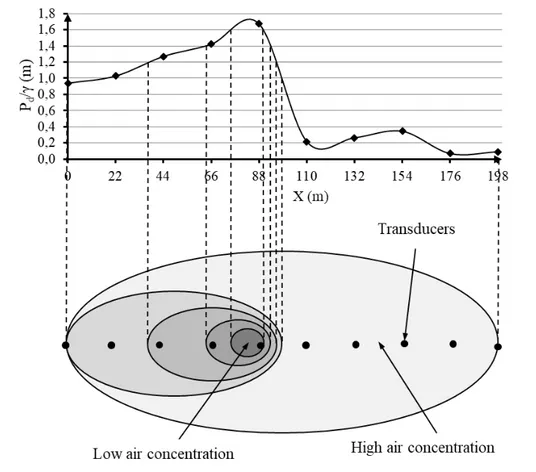
Since Vj was measured from the lip of the flip bucket, the area of the water at the bucket lip was easily calculated by dividing the discharge to the lip velocity. Since the flow area at the bucket lip was known, the rest of the area at the impingement can then be assumed asfull of air. Additionally,

dynamic pressure is inversely proportional with the air ratio, determination of the air percentages depending on dynamic pressure levels at the impingement can be possible (Figure 8).

(a)

Figure 8 Determination of air concentration with respect to dynamic pressure levels

Percentage of the air concentration at the impingement area depending on the dynamic pressure variations can be calculated by using the equation given below.

𝐴𝐴𝑠𝑠𝐴𝐴 % = (𝜕𝜕𝑑𝑑/𝛾𝛾)𝑚𝑚𝑖𝑖𝑚𝑚_(𝜕𝜕∗ (𝐴𝐴𝑠𝑠𝐴𝐴%)𝑚𝑚𝑚𝑚𝑚𝑚

𝑑𝑑/𝛾𝛾)

(9) where Pd/γ is the dynamic pressure head at the impingement point. Due to inverse proportion between the air and water percentages, the air concentration is assumed to be 100% where the dynamic pressure is zero. The rest of the air concentrations are calculated depending on the mentioned fact.

4. Results and Discussions

4.1. Comparison of the Measured, Calculated and Simulated Trajectory Lengths

The following data are measured from the conducted experiments for 6 different cases to determine the trajectory lengths using Kawakami’s equations [14] (Table 2).

Table 2 Measured data from the test cases Discharge for the test cases,

Q (m3_/s) Water depth on the bucket _{lip, hj (m)} Water jet velocity at the bucket _{lip, Vj (m/s)}

0.22 0.035 7.86 0.19 0.031 7.66 0.16 0.027 7.41 0.13 0.023 7.07 0.10 0.019 6.58 0.07 0.015 5.83

To use the provided empirical equations by Kawakami [14], Froude similarity law is applied to find equivalent prototype velocities of the model jet velocities for 1:25 scaled hydraulic model (Table 3).

Table 3 Prototype jet velocities obtained by using Froude similarity law Q (m3_{/s) Vj (m/s) Vjprototype (m/s)} 0.22 7.86 39.29 0.19 7.66 38.31 0.16 7.41 37.04 0.13 7.07 35.33 0.10 6.58 32.89 0.07 5.83 29.17

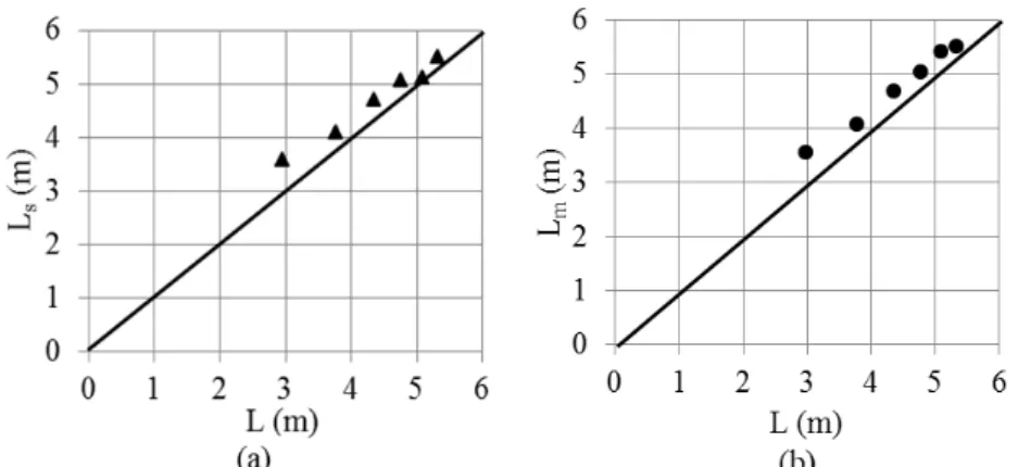
The correctness of the numerical solution can then be checked by comparing with the empirical calculations and experimental measurements. Since this study deals with the air concentration of the water jet from flip bucket at impingement area, measured trajectory lengths from the experiments, calculated trajectory lengths from Kawakami’s equation and simulated trajectory lengths derived from FLOW 3D should be examined first. Cross tabulation of the trajectory lengths for all test cases can be seen in Figure 9.

Figure 9 Cross tabulation of (a) simulated-calculated and (b) measured-calculated trajectory lengths Lm is the measured trajectory length from the model and Ls is the simulated trajectory length obtained from the numerical solutions. Although there are many assumptions in numerical software and analytical calculation, and randomness in measurements, the deviations between the trajectory lengths assumed to be reasonable. Coincidence of the calculated, measured and simulated trajectory lengths show that, positioning of the pressure transmitters depending of the calculated trajectory lengths is applied properly and dynamic pressure measurements are assessed to be reliable for the selected experimental cases.

4.2. Comparison of the Measured and Numerical Dynamic Pressures

Dynamic pressures are measured using pressure transmitters at the impingement area and shown in the figures above. Numerical dynamic pressure values are also obtained after the simulations in FLOW-3D for 6 different discharges. Comparison of the numerical and experimental maximum dynamic pressure values can be seen in Figure 10.

Figure 10 Comparison of the numerical and experimental maximum dynamic pressure values

Pnum and Pexp are the numerical and experimental maximum dynamic pressures for each test case,

respectively. Maximum dynamic pressures are compared to obtain more reliable data from numerical and experimental studies. Consistency between the experimental and numerical dynamic pressures shows that both data can be used to determine air concentration in ski jump jets.

4.3. Air Concentration in Ski Jump Jet

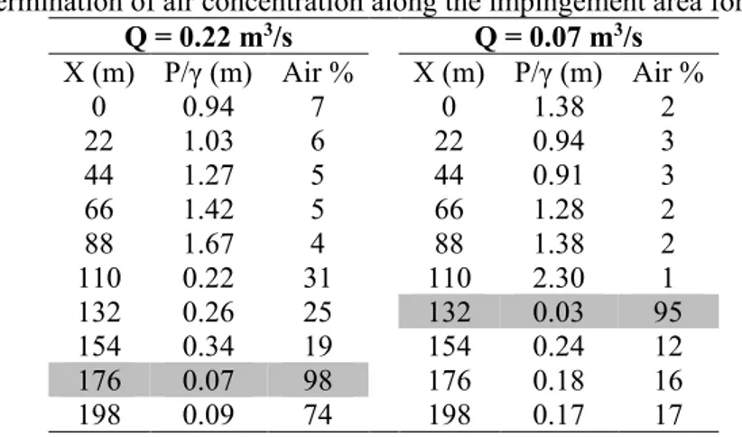
Since air concentration of the jet is inversely proportional with dynamic pressure of the jet as mentioned before, it is easy to calculate the distribution of the air percentage into the water jet from flip bucket. It is assumed that the air concentration is 100% where the dynamic pressure is 0, and 0% when the dynamic pressure is maximum. Related results are given in Table 4.

Table 4 Determination of air concentration along the impingement area for two test cases

Q = 0.22 m3_{/s Q = 0.07 m}3_/s X (m) P/γ (m) Air % X (m) P/γ (m) Air % 0 0.94 7 0 1.38 2 22 1.03 6 22 0.94 3 44 1.27 5 44 0.91 3 66 1.42 5 66 1.28 2 88 1.67 4 88 1.38 2 110 0.22 31 110 2.30 1 132 0.26 25 132 0.03 95 154 0.34 19 154 0.24 12 176 0.07 98 176 0.18 16 198 0.09 74 198 0.17 17

Hence, the concentration of the air absorbed from the medium can be determined in accordance with the dynamic pressure variations at impingement area for the test cases.

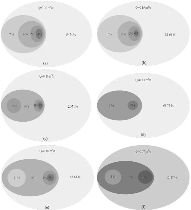
However, when trajectory jet impinged the ground, jet may jump at some points after hitting the impingement area. So, dynamic pressure values can be very low owing to this situation as shown in Table 4 with highlighted rows. To abstain from this occurrence, the point where the lowest dynamic pressure value is obtained can be neglected to obtain more reliable data for air concentration of the water jet. Determination of the air concentration amount into the impinging jet and dynamic pressure variations are calculated based on this fact. So as to determine aeration concentration into the jet coming from the flip bucket, aeration percentages are distributed according to the dynamic pressure head at the impingement points (Figure 11).

Figure 11Air concentration percentage in the impinging jet for all test cases

5. Conclusions

This study deals with air concentration amount of ski jump jet from flip bucket at impingement area in uncontrolled section which is one of the most complex problem in civil engineering. Dispersion of the jet into the air and relationship between the dynamic pressure and air concentration are investigated for 6 different discharges experimentally. Trajectories are determined using three different methods by measuring from the test facility, calculating with empirical equations and obtaining from the numerical runs. All these experimental and numerical data are compared with each other and the following conclusions can be drawn:

i. Air concentration of the water jet can be higher in prototypes than model studies due to much more higher discharges.

ii. Trajectory lengths are affected from air entrainment which shows considerably high energy dissipation into the water jet after the flip bucket of spillway.

iii. Numerical and experimental solutions are almost matching up for the selected test cases. This can be a good method to determine the air concentration into the water jet especially in uncontrolled section using simple equations and assumptions.

iv. Significant increase in dynamic pressures can be observed for jet discharges less than 0.130 m3_{/s. This behavior was partly attributed to low air concentration, a result of small jet velocities at the}

lip of the bucket and can be result of a scale effect for low discharge values.

Acknowledgement

This experimental study was conducted on Laleli Dam and Hydroelectric Power Plant model built for DSIM Projects in Middle East Technical University Hydromechanics Laboratory. The author wants to express deepest gratitude to Prof. Dr. Mustafa M. Aral for his valuable guidance, patience, encouragement and support to completion of this study.

Abbreviations

Atotal : Elliptic area at impingement point (m2)

Aw : Water area at impingement point (m2)

Aa : Air area at impingement point (m2)

a : Width of the dispersed jet at impingement point (m) b : Length of the dispersed jet at impingement point (m) g : Gravitational acceleration (m2_/s)

ρ : Density

hj : Water depth on the bucket lip (m)

Vm : Model velocity (m/s)

Vp : Prototype velocity (m/s)

Lm : Measured Trajectory length (m)

Ls : Simulated Trajectory length (m)

L : Calculated Trajectory length (m) k : Constant related to air resistance Q : Water discharge (m3_/s)

Pd/γ : Dynamic pressure head (m)

Vj : Velocity at the bucket lip (m/s)

w : Channel width (m)

zi : Vertical drop from lip to tail-water level (m)

α : Trajectory length constant from Equation 2 αj : Flip bucket lip angle (degree)

γ : Specific weight of water (N/m3₎

X : Distance of the pressure transmitter from the bucket lip (m) τij : Reynold’s Stress

Fr : Froude Number

Kaynaklar

[1] Carrillo JM, Castillo LG, Marco F, García JT. Experimental and numerical analysis of two-phase flows in plunge pools. Journal of Hydraulic Engineering 2020; 146(6).

[2] Sarwar MK, Ahmad I, Chaudary ZA, Mughal HUR. Experimental and numerical studies on orifice spillway aerator of Bunji Dam. Journal of the Chinese Institute of Engineers 2020; 43(1): 27-36.

[3] Li S, Zhang J, Xu W. Numerical investigation of air–water flow properties over steep flat and pooled stepped spillways. Journal of Hydraulic Research 2018; 56(1): 1-14.

[4] Dong Z, Wang J, Vetsch DF, Boes RM, Tan G. Numerical Simulation of Air–Water Two-Phase Flow on Stepped Spillways behind X-Shaped Flaring Gate Piers under Very High Unit Discharge. Water 2019; 11(10): 1956.

[5] Li S, Yang J, Li Q. Numerical Modelling of Air-Water Flows over a Stepped Spillway with Chamfers and Cavity Blockages. KSCE Journal of Civil Engineering 2020; 24(1): 99-109.

[6] Juon R, Hager WH. Flip bucket without and with deflectors. Journal of Hydraulic Engineering 2000; 126(11): 837-845.

[7] Tsen-ding C. ON The Energy Dissipation of High Overflow Dam with Flip Bucket and Estimation of Downstream Local Erosion. Journal of Hydraulic Engineering 1963; 2.

[8] Khatsuria RM. Hydraulics of Spillways and Energy Dissipators, CRC Press, Taylor & Francis Group, NW, 2005; ISBN: 978-0-203-99698-0.

[9] Rajan BH, Shivashankara Rao KN. Design of trajectory buckets. J. Irrig. Power India 1980; 37(1): 63–76, ISSN : 0974-4711.

[10] Heller V, Hager WH, Minor HE. Ski jump hydraulics, J. Hydraul. Eng. 2005; 131(5):347–355, DOI:10.1061/(ASCE)0733-9429(2005)131:5(347).

[11] Steiner R, Heller V, Hager WH, Minor HE. Deflector ski jump hydraulics, Journal of Hydraulic Engineering 2008; 5(134): 562-571, DOI: 10.1061/(ASCE)0733-9429(2008)134:5(562).

[12] Chanson H. Air Bubble Entrainment in Turbulent Water Jets Discharging into the Atmosphere, Australian Civil/Structural Engineering Transactions 1996; 1(39).

[13] Schmocker L, Pfister M, Hager WH, Minor HE. Aeration characteristics of ski jump jets, ASCE Journal. of Hydraulic Engineering 2008; 134(1):90-97.

[14] Kawakami K. A Study on the Computation of Horizontal Distance of Jet Issued from Ski-Jump Spillway, Proceedings of the Japan Society of Civil Engineers 1973; 1973(219):37-44, Doi: http://doi.org/10.2208/jscej1969.1973.219_37.

[15] Aydin I, Göğüş M, Altan-Sakarya AB, Köken M. Laleli Dam and HEPP Spillway Hydraulic Model Studies, Hydromechanics Laboratory, Civil Engineering Department, 2012, METU. [16] Data Acquisition (DAQ) Software retrieved from: http://turkey.ni.com/

[17] Launder BE, Spalding DB. The numerical computation of turbulent flows, Computer Methods in Applied Mechanics and Engng. 1974; 3(2):269–289, DOI:10.1016/0045-7825(74)90029-2. [18] Wilcox DC. Turbulence modelling for CFD, DCW Industries, Inc. 2000, La Canada CA, DOI:

10.1017/S0022112095211388.

[19] Zhang N, Chato DJ, McQuillen JB, Motil BJ, Chao DF. CFD simulation of pressure drops in liquid acquisition device channel with sub-cooled oxygen, World Academy of Science, Engineering and Technology 2012; 58:1180-1185, DOI: 10.1016/j.ijhydene.2014.01.035.

[20] Speziale CG. Analytical methods for the development of Reynolds-stress closures in turbulence, Annual Review of Fluid Mechanics 1991; 23:107–157, DOI: 10.1146/annurev.fl.23.010191.000543.

[21] Flow 3D, v10.1 User Manuel, 2012, Available

at:http://www.easysimulation.com/public/flow3dcast/documentation/FLOW-3D_Cast_3.2_Manual.pdf