Explaining the Gender Wage Gap in Turkey
Using the Wage Structure Survey
BETAM WORKING PAPER SERIES #005
Explaining the Gender Wage Gap in Turkey
Using the Wage Structure Survey
∗
Arda Aktas
†and Gokce Uysal
‡March 13, 2012
Abstract
Gender discrimination in the labor market can take on many forms, the most prominent one being the gender gap in wages. The labor market in Turkey is not an exception. Even though the gender wage gap is 3 percent on average, a closer look reveals important differences along the wage distribution. There is virtually no gender gap at the lower end and men earn 6.47 percent more than women at the median. Surprisingly, women seem to earn 4.99 per-cent higher wages than men at the top of the wage distribution. Using the quantile regression method, we discuss how the labor market returns differ along the wage distribution. Secondly, we use the Machado-Mata decomposition method to reveal how much of the gender gap at each quantile can be explained by gender differences in characteristics versus gender differences in returns. We find that the gender gap actually widens when we control for basic characteristics such as age, education and tenure. In other words, controlling for gender differences in labor market characteristics reveals that there is gender discrimination in Turkey, as measured by the differences in returns.
Keywords: Gender wage gap, Machado-Mata Decomposition,Quantile Regression
1
Introduction
Wages have been elaborately studied to reveal gender discrimination in labor markets in many countries around the world. The early studies on the gender gap in wages focus on the differences in mean wages. More recent research has concentrated on studying the gender wage gap along the entire wage distribution and has shown that gender discrimination may differ along the wage distribution. In some countries, women face glass ceilings as manifested by larger gender gaps at the top of the wage distribution. In others, women are standing on stick floors where gender gaps ∗We are grateful to Seyfettin Gursel, Zumrut Imamoglu and Duygu Guner for valuable comments. All errors are
our own.
†State University of New York at Stony Brook, [email protected]
‡Corresponding author,Bahcesehir University Center for Economic and Social Research,
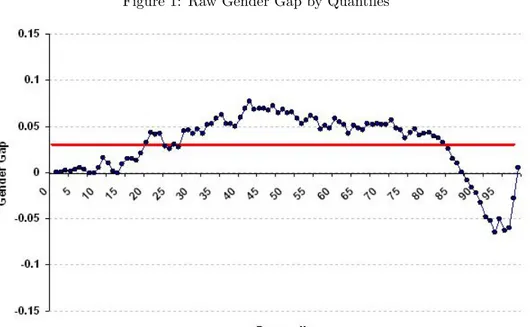
Figure 1: Raw Gender Gap by Quantiles
are decreasing at the bottom of the wage distribution. Following this strand, we study the gender gap along the wage distribution in Turkey.
Looking at mean wages, the gender wage gap in Turkey is around 3 percent. However, gender differences in wages are not uniform across the wage distribution. Figure 1 plots the gender wage gap at different percentiles. The gender wage gap seems to fluctuate around zero at the very low end of the distribution. This indicates that the sticky floor may be an important phenomenon in the labor market in Turkey. The gender gap increases to about 6.47 percent at the median. At the top of the wage distribution, we observe a sharp decrease in the gender gap. It even changes sign around the 90th percentile. The gender gap becomes negative 6.49 percent at the 94th percentile. In other words, let along a glass ceiling, the data indicates that that men may actually be earning lower wages than women at the very top of the distribution. It is only on the 99th percentile that the gender gap turns positive again.
Why does the gender gap vary along the wage distribution? Are the characteristics of males and females very different or are labor market returns very different at different quantiles? We use the the quantile regression technique to study the labor market returns at different quantiles of the wage distribution. We run regressions on the entire sample as well as on female and male samples separately. The quantile regression results indicate that labor market returns are different at different quantiles and also that there are gender differences in labor market returns. Regression on a pooled sample of females and males show that when we use basic controls such as education, age and tenure, the gender gap becomes wider all throughout the distribution. The most striking effect occurs at the top end. We find that women’s wages are about 4.5 percent below those of men above the 90th percentile when we control for basic characteristics. The sticky floor pattern
changes as well, the gender gap increases at the low end of the distribution. As a second step, we include controls on arguably endogenous characteristics such as industry, occupation, firm size, administrative posts and collective bargaining. These help explain some part of the gender gap across the wage distribution.
The next question is how much of the gender gap can be attributed to differences in characteristics and how much to differences in labor market returns to these characteristics? More importantly, does this depend on the quantiles? To decompose the gender wage gap at various quantiles, we use the Machado-Mata decomposition technique. We find that after controlling for basic characteristics, the part of the gender gap that stems from differences in returns are larger than the observed gender gap. In other words, differences in characteristics actually hide the true size of the gender gap stemming from differences in returns.
The paper is organized as follows. In Section 2 we provide a brief summary of the related literature. In Section 3 and Section 4, we describe the data set we use, and provide the descriptive statistics as well as the methodology used. Section 5 and 6 present the results of the wage regressions and the decomposition. Section 7 concludes.
2
Literature Survey
The earlier literature that studies the gender wage gap consists of least squares regressions and Blinder (1973) - Oaxaca (1973) decomposition. These methods concentrate on the mean of the wage distribution, hence provide a limited understanding of the gender gap. Therefore, several other methods have been developed to study the gender gap along the wage distribution.
Albrecht et al. (2003) are one of the first to study the gender gap along the wage distribution using quantile regression and Machado and Mata (2005) decomposition techniques. They find that the differences in returns to labor market characteristics constitute a major part of the gender gap in wages. Moreover, they find evidence of a strong glass ceiling effect in Sweden. That is, the gender wage gap is much wider at the top of the distribution when they control for covariates such as age and education.
Arulampalam et al. (2007) study the gender wage gap for 11 countries in Europe using the quantile regression techniques to study the gender wage gap along the wage distribution as well as the Machado-Mata decomposition technique. They find that the women would have been paid less even if they had had men’s characteristics. Moreover, the results indicate that in Belgium, Finland, France, Italy and Spain, women typically have better characteristics than men. In other words, the differences in wages due to differences in returns are sizeable and sometimes even more than the observed gender gap itself.
Using Spanish data, Rica et al. (2008) document the existence of a glass ceiling as well as a sticky floor. They find that the gender wage gap increases along the wage distribution for college graduates in Spain. On the other hand, the gender gap decreases for low education groups. The authors label this as a sticky floor and argue that it could be an implication of statistical discrimination. There are few studies that examine the gender wage gap in the labor market in Turkey. This is mainly due to the fact that large, reliable data sets that contain information on labor market status
have only recently been shared with public. Moreover, all of these studies concentrate on the mean gender gap and its decomposition. Ours is the first study that studies the gender wage gap along the entire wage distribution.
Dayıoˇglu and Kasnakoˇglu (1997) examine gender based wage differentials in urban Turkey by using Household Income and Expenditure Survey (HIES) of 1987. The mean gender wage gap is 4 percent for wage earners in their data set. This is similar to the wage gap we find. They conduct a Blinder (1973) - Oaxaca (1973) type decomposition and attribute at least 63.8 percent of gender wage differentials to discrimination. The authors also note that using female coefficients in the decomposition, the gender gap increases to 100 percent. Our results are also parallel, we also find a larger discrimination component when female returns are used.
Using the Household Labor Force Survey of 1988 and 1994, Dayıo˘glu and Tunalı (2004) document a gender wage gap of 2 and 15 percent respectively. The authors run basic wage regressions as well as wage regressions that control for sample selection. They point out that controlling for sample selection increases the discrimination component in 1988 and reduces it in 1994. They also point to a higher discrimination component when they use female returns in the Blinder (1973) - Oaxaca (1973) type decomposition.
Tansel (2003) examines formal and informal wage earners as well as the self-employed using the 1994 Turkish Household Expenditure Survey. The gender wage gap is at 26.59 percent Using a multinomial logit to control for sample selection, the author finds that the gender gap expands to 47.73 percent from 26.59 percent among the wage earners in the formal sector when all controls are included. The results indicate that selection accounts for about half of the gender gap and the part attributed to discrimination is about 36.62 percentage points.
Using the same data set, Tansel (2005) studies the gender based wage differentials in the public sector, state owned firms (SOEs) and the formal private wage sector in Turkey. The results show that there exists a gender gap in wages in the SOEs (18 percent) and in the private sector (26 percent), while the gender gap is almost nonexistent (0.2 percent) in the public sector. Using the Blinder (1973) - Oaxaca (1973)decomposition method, Tansel (2005) finds that the unexplained part of gender wage gap is higher and negative in the private sector. This result implies that gender discrimination may be more severe in the private sector.
Ilkkaracan and Selim (2007) study the gender wage gap in Turkey by using Employment and Wage Structure Survey for 1994. They conduct OLS regressions followed by a Blinder (1973) - Oaxaca (1973) decomposition. The gender gap in their sample is 0.3485. The authors point out that their sample is based on firm-level data from manufacturing, electricity, gas and water, mining and quarrying sectors, thus may overestimate the gender gap in the overall economy. The Oaxaca decomposition results indicate that the unexplained part of the gender gap, i.e. the part attributed to discrimination, is 43 percent when only human capital variables are used, and drops to 22 percent with the inclusion of workplace variables. The gender gap drops to 9.2 percent when they include all controls.
Cudeville and Gurbuzer (2010) use 2003 Household Budget Survey to study the gender gap in the labor market in Turkey. The raw gender gap in their data is 25.2 percent. However, once the authors restrict the sample to full time wage earners, the raw gender gap comes down to 10.4 percent. Even though they point out that the gender gap is not uniform across the wage
distribution, the authors run a Mincerian wage equation followed by a Blinder (1973) - Oaxaca (1973) decomposition. Their findings indicate that at least 46 percent of the wage differences are due to discrimination. Controlling for basic characteristics increases the part due to discrimination to 76 percent. The authors point out that controlling for selection does not alter their findings drastically.
The gender gap in our sample is clearly much smaller than some of those cited in the literature for Turkey. We believe that the discrepancy is caused by the data set used. The Wage Structure Survey, as explained below, is not representative of employment in Turkey. However, it provides a good data set for studying the gender gap along the entire wage distribution given that it is much larger than all other data sets. As far as we know, ours is the first study on the labor market in Turkey that studies the gender gap along the wage distribution using the quantile regression methodology coupled with the Machado-Mata decomposition.
3
Data and Descriptive Statistics
3.1
Wage Structure Survey
The data used for the analysis in this paper is from the Wage Structure Survey conducted by TURKSTAT. Wage Structure Survey is a firm-based data set which provides detailed information on workers’ wages, workers’ demographic characteristics as well as firm characteristics. The wages are measured in November 2006 YTL. Since the data is collected at the firm level, it consists of formally employed workers only, and thus fails to cover the employees in the informal sector. According to data from the Household Labor Force Survey 2006, 33.4 percent of men and 35.3 percent of women in non-agricultural sectors are not registered at the Social Security Institution. Moreover, Wage Structure Survey is conducted in firms that have at least 10 workers. Again, according to data from the Household Labor Force Survey 2006, 47.6 percent of men and 61.4 percent of women work in firms that have at least 10 workers. Put differently, the Wage Structure Survey contains data on 41.3 percent of total male and 51.9 percent of total female workers in the non-agricultural labor market.
Despite its shortcomings, Wage Structure Survey is the largest data set that provides information on wages: there are more than 300 thousand employees in the data set.1 It contains detailed industry and occupation information as well as information on administrative posts and collective bargaining.
3.2
Our sample
In order to make the sample more homogenous, we restrict our analysis to employees working full time, i.e. those paid at least 30 hours per week excluding overtime in November 2006. The percentage of employees working full time corresponds to 99.3 of the full sample.
The wages are taken as earnings in November 2006 YTL. In Turkey, a majority of the workers are 1A typical year of Household Labor Force Survey has about 150 thousand observations.
paid on a monthly basis. So, the dependent variable is the logarithm of gross monthly wage. As stated above, Wage Structure Survey does not contain any information on the actual work histories of individuals, such as actual work experience. Potential work experience is constructed in the usual way.2
Upon first inspection of the data, underreporting of wages appears to be a serious concern. Ap-proximately one third of the employees in our data set seem to be employed at the minimum wage, which was 531 TL in 2006. The data from the Household Labor Force Surveys indicates that only 17.3 percent of the employed who work full time formally for firms with at least 10 employees in 2006 earn between 500 TL and 600 TL per month.3 However, note also that the same data shows that even though they were working formally and full time, 25.7 percent of the wages were below 500 TL.4
It is common practice in Turkey for firms to report employee wages at the minimum wage to avoid taxes. In 2006, both the employer contribution to social security taxes and severance pay were high, making formal employment costly for employers.It may well be the case that the firms were paying taxes as if the employees were employed at the minimum wage and compensating the employees informally. Since it is impossible to identify who was actually paid minimum wage and whose wage was underreported, we choose to exclude these employees from the analysis. Of course, if the employers are more likely to register females at the minimum wage than males, this will cause the gender gap to appear smaller than the data indicates. However, those employed at the minimum wage make up 32.6 percent of the females and 33.7 percent of the males in the data set. In other words, excluding those who make minimum wage in the data set, excludes relatively more males than females.
3.3
Descriptive Statistics
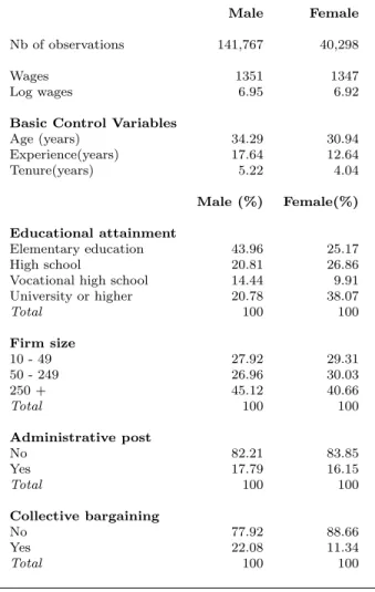
Descriptive statistics are provided in Table 1. Note that there are important differences in char-acteristics of males and females. The females are younger and therefore they have lower levels of potential job market experience and tenure. However, females in employment have much higher education levels compared to males: 38.07 percent of females have at least a college degree whereas only 20.78 percent of males do.5 26.86 percent of females are general high school graduates com-pared to 20.81 percent of males. Vocational school graduates constitute 9.91 percent of females and 14.44 percent of males in our sample.
There are similar albeit less pronounced differences in other control variables. Females tend to work for smaller firms. Moreover, they are less likely to be covered by collective bargaining agreements and less likely to hold administrative posts.
Raw data indicates that the gender gap is 3 percent. To get a clear idea of differences along the the 2Potential experience is equal to age minus years of schooling, minus the age at which children start school, which
is equal to 7 in Turkey.
3Since the Household Labor Force Surveys are collected at the household level, we believe that there is less
underreporting of wages.
4These workers may have worked full time, but for less than one month.
5Low LFPR of women in Turkey coupled with high LFPR for college graduates imply that the females in
Table 1: Descriptive Statistics
Male Female Nb of observations 141,767 40,298
Wages 1351 1347
Log wages 6.95 6.92 Basic Control Variables
Age (years) 34.29 30.94 Experience(years) 17.64 12.64 Tenure(years) 5.22 4.04 Male (%) Female(%) Educational attainment Elementary education 43.96 25.17 High school 20.81 26.86 Vocational high school 14.44 9.91 University or higher 20.78 38.07 Total 100 100 Firm size 10 - 49 27.92 29.31 50 - 249 26.96 30.03 250 + 45.12 40.66 Total 100 100 Administrative post No 82.21 83.85 Yes 17.79 16.15 Total 100 100 Collective bargaining No 77.92 88.66 Yes 22.08 11.34 Total 100 100
Male (%) Female(%) Industry
C Mining and quarrying 2.45 0.40 DA Manufacture of food products, beverages and tobacco products 5.11 2.96 DB Manufacture of textiles and textile products 12.01 20.29 DC Manufacture of leather and leather products 0.82 0.59 DD Manufacture of wood and wood products 0.53 0.17 DE Manufacture of pulp, paper and paper products; publishing and printing 1.85 1.24 DF Manufacture of coke, refined petroleum products and nuclear fuel 0.46 0.28 DG Manufacture of chemicals, chemical products and man-made fibres 2.53 2.29 DH Manufacture of rubber and plastic products 1.93 0.88 DI Manufacture of other non-metallic mineral products 3.84 1.75 DJ Manufacture of basic metals and fabricated metal products 7.78 2.03 DK Manufacture of machinery and equipment n.e.c. 4.67 1.99 DL Manufacture of electrical and optical equipment 2.72 3.24 DM Manufacture of transport equipment 4.43 1.20 DN Manufacturing n.e.c. 1.67 1.66 E Electricity, gas and water supply 2.54 0.75
F Construction 4.87 2.20
G Wholesale and retail trade; repair of motor vehicles and motorcycles 13.91 17.02 H Hotels and restaurants 3.65 3.48 I Transport, storage and communication 9.53 8.79 J Financial intermediation 1.92 5.32 K Real estate, renting and business activities 5.65 6.75
M Education 2.03 6.71
N Health and social work 1.33 6.42 O Other community, social and personal service activities 1.76 1.59
Total 100 100
Occupation (ISCO 2 digits)
11 Legislators and Senior Officials 0.02 0.01
12 Corporate Managers 5.77 5.58
13 General Managers 0.5 0.37
21 Physical, Mathematical and Engineering Science Professionals 2.93 2.67 22 Life Science and Health Professionals 0.54 1.73 23 Teaching Professionals 1.04 4.9 24 Other Professionals 2.27 5.94 31 Physical and Engineering Science Associate Professionals 6.65 4.82 32 Life Science and Health Assocaite Professionals 0.62 2.81 33 Teaching Associate Professionals 0.04 0.21 34 Other Associate Professionals 9.21 14.84
41 Office Clerks 7.33 14.4
42 Customer Services Clerks 1.61 6.17 51 Personal and Protective Services Workers 5.82 3.15 52 Models, Salespersons and Demonstrators 2.84 4.26 61 Market-Oriented Skilled Agricultural abd Fishery Workers 0.36 0.09 71 Exraction Building Trades Workers 4.42 0.39 72 Metal, Machinery and Related Ttrades Workers 8.9 1.94 73 Precision, Handicraft, Printing and Related Trades Workers 2.24 1.39 74 Other Craft and Related Trades Workers 6.53 8.14 81 Stationary-Plant and Related Operators 2.75 0.5 82 Machine Operators and Assemblers 8.97 6.2 83 Drivers and Mobile-Plant Operators 5.16
91 Sales and Services Elementary Occupations 4.94 5.22 92 Agricultural, Fishery and Related Labourers 0.07 0.04 93 Labourers in Mining, Construction, Manufacturing and Transport 8.48 4.24
wage distribution, Figure 2 presents the gender gaps at each percentile. First, concentrate on the graph on the upper left hand side, which plots the observed gender gap at different percentiles. This is the same as Figure 1. Note that even though the mean gender gap is around 3 percent (6.92 for females vs. 6.95 for males), the gender gap exhibits some differences along the wage distribution. It starts around zero at the lower tail, and stays there for the lowest quintile, after which it starts decreasing slowly. It reaches its peak of 7.74 percent at the 42nd percentile and decreases very slowly until the upper tail of the distribution. From the 85th percentile on, we observe a steeper descent in the gender gap, and it even turns positive after the 90th percentile. Said differently, raw data indicates that women in the upper tail of the wage distribution have higher wages than men. Remember women in our sample are more educated than men. In other words, especially at the top end of the wage distribution, women are much more likely to be college graduates. Therefore, they may have higher wages just because the returns to college are higher than the returns to high school. To see whether this may be the case, we plot the gender gap at all percentiles by education levels in Figure 2.
Let us concentrate on the gender gap for college graduates. Observe that is is almost zero at the lower end of the distribution, up to the 5th percentile. However, it starts increasing consistently as we move up the distribution. Having reached 20 percent around the median, it stagnates at that level until the 70th percentile after which it increases slightly again. Even though there is a minor decrease around the 85th percentile, the gender gap barely goes below 20 percent, it even surpasses 20 percent after the 90th percentile. Clearly, a gender gap exists for the college graduates, is sizeable and persistently increasing along the wage distribution.
The gender gap for high school graduates exhibits a similar pattern along the wage distribution, except for the fact that towards the upper tail, the gender gap decreases considerably. We believe that this decrease may be due to the selection into the labor market. Since many of the women drop out when they are married or have children, we would expect those who stay to earn higher wages, implying higher wages for women. Clearly, given increasing age-wage profiles, we would expect this selection to be more noticeable at the top of the distribution.
A strikingly different figure emerges for the elementary school graduates. The gender gap increases fast as we move up the wage distribution. It reaches 50 percent around the 90th percentile, and then it drops sharply. Note that the number of females in this category in our sample is merely 8,526 whereas there are 60,098 males. Females with only an elementary education degree constitute a much larger share of the working age female population. In other words, we expect selection into the labor market to be much stronger for elementary school graduates.
Figure 2 provides clear evidence that the gender gap varies considerably across the wage distribution, hence calls for an econometric method that allows us to do that. Next section summarizes the quantile regression methods that we use in this paper to study the gender gap.
4
Methodology
The early studies on the gender wage gap use OLS regression techniques to study the gender wage gap. By construction, these methods focus on the mean of the wage distribution. That is,
Figure 2: Gender Gap b y Quan tiles
the marginal returns to characteristics are estimated only at the mean. More recently, quantile regression techniques have been used for studying the marginal effects of the covariates on log wages at different quantiles of the wage distribution.
Quantile regression techniques are based on estimating the θth quantile of log wages (ln w) condi-tional on covariates (x). The coefficient vector is the vector that minimizes the sum of absolute errors. min β (θ) X i:ln wi≥xiβ(θ) θ |ln wi− xiβ (θ)| + X i:ln wi<xiβ(θ) (1 − θ) |ln wi− xiβ (θ)|
5
Results
5.1
Pooled Regressions
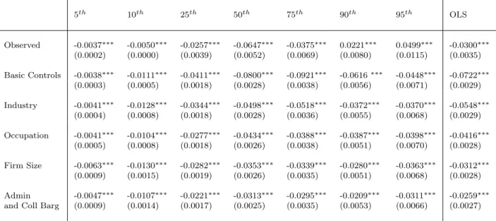
Using the quantile regression techniques, we study the gender gap at specific percentiles along the wage gap. To begin with, we assume that the males and the females have the same returns in the labor market, i.e. we run regressions with a pooled data set of males and females, and introduce a female dummy in the regressions. Table 2 presents the gender gap at the 5th, 10th, 25th, 50th, 75th, 90th and 95th percentiles for different specifications.
The first row marks the raw gender gap at the given percentiles. Consistent with Figure 2, we observe that the raw gender gap starts very close to zero (0.37 percent), increases in absolute value until -6.47 percent at the median, then decreases and eventually turns positive at the 90th (2.21 percent) and 95th percentiles (4.99 percent).6 In other words, the female dummy has a positive coefficient in a simple regression of log wages: At the very top of the distribution, female wages are higher than male wages. Also note that the OLS coefficient is significantly negative at −3 percent. In the second panel, we control for basic labor market characteristics: age, age squared, tenure, tenure squared and educational attainment. The gender gap increases in absolute value relative to the observed gender gap. Remember that the females in our sample are better educated than males. In other words, at a given quantile of the wage distribution, the education level of a female is higher than that of a male. Therefore, controlling for education, we observe that the gender gap actually widens. The widening of the gender gap starts from the 10th percentile up and becomes more pronounced at and above the median. The gender gap expands from -6.47 percent to -8 percent at the median, from -3.75 percent to -9.21 percent on the 75th percentile. The OLS estimate also expands sizeably, from -3 percent to -7.22 percent. Consistent with Figure 2, the gender gap turns negative at the top end of the wage distribution. That is, we find that women earn lower wages when we control for education. At the 90th percentile, the gender gap changes sign from 2.21 percent to -6.16 percent, at the 95th, from 4.99 percent to -4.48 percent.
6These are the coefficients on a dummy that assigns the value 1 to females, in other words, a negative number
indicates that females earn less than males. For example, -6.47 percent implies that females earn 6.47 percent less than their male counterparts at the median. 4.99 percent implies that females earn 4.99 percent more than their counterparts at the 95th percentile.
Table 2: Estimates of the Gender Wage Gap Using Pooled Data (n=182,075) 5th 10th 25th 50th 75th 90th 95th OLS Observed -0.0037∗∗∗ -0.0050∗∗∗ -0.0257∗∗∗ -0.0647∗∗∗ -0.0375∗∗∗ 0.0221∗∗∗ 0.0499∗∗∗ -0.0300∗∗∗ (0.0002) (0.0000) (0.0039) (0.0052) (0.0069) (0.0080) (0.0115) (0.0035) Basic Controls -0.0038∗∗∗ -0.0111∗∗∗ -0.0411∗∗∗ -0.0800∗∗∗ -0.0921∗∗∗ -0.0616∗∗∗ -0.0448∗∗∗ -0.0722∗∗∗ (0.0003) (0.0005) (0.0018) (0.0028) (0.0038) (0.0056) (0.0071) (0.0029) Industry -0.0041∗∗∗ -0.0128∗∗∗ -0.0344∗∗∗ -0.0498∗∗∗ -0.0518∗∗∗ -0.0372∗∗∗ -0.0370∗∗∗ -0.0548∗∗∗ (0.0004) (0.0008) (0.0018) (0.0028) (0.0036) (0.0055) (0.0068) (0.0029) Occupation -0.0041∗∗∗ -0.0104∗∗∗ -0.0277∗∗∗ -0.0434∗∗∗ -0.0388∗∗∗ -0.0387∗∗∗ -0.0398∗∗∗ -0.0416∗∗∗ (0.0005) (0.0008) (0.0018) (0.0026) (0.0038) (0.0051) (0.0070) (0.0028) Firm Size -0.0063∗∗∗ -0.0130∗∗∗ -0.0282∗∗∗ -0.0353∗∗∗ -0.0339∗∗∗ -0.0280∗∗∗ -0.0363∗∗∗ -0.0312∗∗∗ (0.0009) (0.0015) (0.0019) (0.0026) (0.0035) (0.0051) (0.0068) (0.0028) Admin -0.0047∗∗∗ -0.0107∗∗∗ -0.0221∗∗∗ -0.0313∗∗∗ -0.0295∗∗∗ -0.0209∗∗∗ -0.0311∗∗∗ -0.0259∗∗∗ and Coll Barg (0.0009) (0.0014) (0.0017) (0.0025) (0.0035) (0.0053) (0.0066) (0.0027) Standard errors in parentheses *** p<0.01, ** p<0.05, * p<0.1
When we include industry dummies in the regressions, we can explain a non-trivial part of the gender gap at and above the median. It shrinks by almost half at the median from 8 percent to 4.98 percent and at the 75th percentile from -9.21 to -5.18. The decreases in the upper part are similar but smaller in size. The gender gap shrinks from -4.48 to -3.70 at the 95th percentile. When occupations are taken into account, we can explain still a little bit more of the gender gap, especially at the 10th, 25th and 75th percentiles. Note that above the median, the gender gap seems almost stable around 3.90 percent. Again, the gender gap is larger around the median, 4.98 percent.
We control for firm size in the next panel of Table 2. It is interesting to see that firm size explains the gender gap above the median although it widens the gender gap below the median. At the 10th percentile, the gender gap widens from 1.04 to 1.30 percent. At the 90th percentile, including firm size in regressions causes the gender gap to shrink from 3.87 to 2.80 percent.
At the last panel, we include controls for administrative posts and collective bargaining coverage. Doing so helps explain the gender wage gap at all quantiles of the wage distribution. However, a considerable gender gap still remains. The gender wage gap increases from the 5th percentile to the median. At and above the median, the gender gap seems pretty stable at 3 percent.
At this point, it is interesting to compare the first and the last panel of Table 2. Including the control variables reduces the gender wage gap at the median, but widens it considerably at the very high end of the distribution. The raw gender gap points to a 4.99 percent higher wages for females whereas the gender gap with all controls points to a 3.11 percent higher wages for males at the 95th percentile. Clearly, the quantile regressions tell a more detailed story than the OLS regressions, even when we assume that the returns to labor market characteristics are the same for males and
females.
5.2
Regressions by Gender
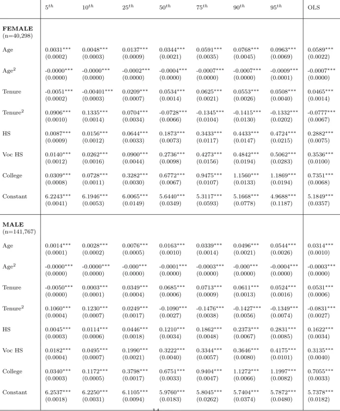
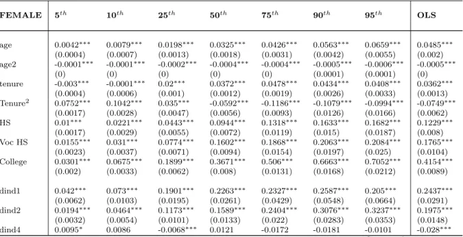
In the previous subsection, we ran pooled regressions assuming that returns to labor market char-acteristics were the same for males and females. In this section, we will concentrate on the gender differences between returns to labor market characteristics. Table 3 provides the quantile regres-sions by gender to study the gender differences in returns to labor market characteristics where we control for basic characteristics of the individual. The coefficients of models where we control for other labor market characteristics are provided in Appendix A.
The coefficients on age are higher for females than for males. Given that in our sample, women are younger than men, it is not surprising that the returns to age, which is a proxy for labor market experience, are higher for females than for males. Moreover, the returns to age are higher in the upper part of the wage distribution regardless of gender. One other finding is that the difference in returns to age between males and females increases as we move up the wage distribution. Returns to tenure are also different for males and females. Males seem to enjoy higher returns to tenure than females do. It is interesting to see that below the median, the returns to tenure are convex. In other words, the higher tenured workers enjoy increasing returns to tenure. However, at and above the median, the returns to tenure are positive but decreasing and at a relatively high rate.
As for education, the returns to a high school diploma increase as we move up the wage distribution. However, they are considerably higher for females than for males. A different pattern is observed for the returns to vocational high school diploma. The returns to vocational high school are higher for males in the lower half of the distribution, they are higher for females in the higher half. The returns to a college degree are really high and increasing over the wage distribution. College education seems to have slightly higher returns for males than for females at almost every quantile. Differences are larger at the low half of the distribution.
The quantile regressions by gender indicate clearly that the returns to labor market characteristics differ for males and females. At this point, it would useful to decompose the gender gap into two parts, one stemming from differences in characteristics, the other from differences in returns.
6
Decomposition Results
The decomposition technique used in this paper has been developed by Machado and Mata (2005). The Machado-Mata decomposition is a natural extension to the Blinder-Oaxaca decomposition for quantile regressions. Just like the Bilnder-Oaxaca decomposition, it holds exactly in this case since the quantile regression is also linear.
Using the Machado-Mata decomposition, we can generate two counterfactual densities: a female log wage density assuming that women had men’s characteristics, but were paid as women (Xmβf) and a male log wage density assuming that men had women’s characteristics, but were paid as men
Table 3: Quantile Regressions by Gender 5th 10th 25th 50th 75th 90th 95th OLS FEMALE (n=40,298) Age 0.0031∗∗∗ 0.0048∗∗∗ 0.0137∗∗∗ 0.0344∗∗∗ 0.0591∗∗∗ 0.0768∗∗∗ 0.0963∗∗∗ 0.0589∗∗∗ (0.0002) (0.0003) (0.0009) (0.0021) (0.0035) (0.0045) (0.0069) (0.0022) Age2 -0.0000∗∗∗ -0.0000∗∗∗ -0.0002∗∗∗ -0.0004∗∗∗ -0.0007∗∗∗ -0.0007∗∗∗ -0.0009∗∗∗ -0.0007∗∗∗ (0.0000) (0.0000) (0.0000) (0.0000) (0.0000) (0.0000) (0.0001) (0.0000) Tenure -0.0051∗∗∗ -0.00401∗∗∗ 0.0209∗∗∗ 0.0534∗∗∗ 0.0625∗∗∗ 0.0553∗∗∗ 0.0508∗∗∗ 0.0465∗∗∗ (0.0002) (0.0003) (0.0007) (0.0014) (0.0021) (0.0026) (0.0040) (0.0014) Tenure2 0.0906∗∗∗ 0.1335∗∗∗ 0.0704∗∗∗ -0.0728∗∗∗ -0.1345∗∗∗ -0.1415∗∗∗ -0.1332∗∗∗ -0.0777∗∗∗ (0.0010) (0.0014) (0.0034) (0.0066) (0.0104) (0.0130) (0.0202) (0.0067) HS 0.0087∗∗∗ 0.0156∗∗∗ 0.0644∗∗∗ 0.1873∗∗∗ 0.3433∗∗∗ 0.4433∗∗∗ 0.4724∗∗∗ 0.2882∗∗∗ (0.0009) (0.0012) (0.0033) (0.0073) (0.0117) (0.0147) (0.0215) (0.0075) Voc HS 0.0140∗∗∗ 0.0262∗∗∗ 0.0900∗∗∗ 0.2736∗∗∗ 0.4273∗∗∗ 0.4842∗∗∗ 0.5062∗∗∗ 0.3536∗∗∗ (0.0012) (0.0016) (0.0044) (0.0098) (0.0156) (0.0194) (0.0283) (0.0100) College 0.0309∗∗∗ 0.0728∗∗∗ 0.3282∗∗∗ 0.6772∗∗∗ 0.9475∗∗∗ 1.1560∗∗∗ 1.1869∗∗∗ 0.7351∗∗∗ (0.0008) (0.0011) (0.0030) (0.0067) (0.0107) (0.0133) (0.0194) (0.0068) Constant 6.2243∗∗∗ 6.1946∗∗∗ 6.0065∗∗∗ 5.6440∗∗∗ 5.3117∗∗∗ 5.1668∗∗∗ 4.9688∗∗∗ 5.1849∗∗∗ (0.0041) (0.0053) (0.0149) (0.0349) (0.0593) (0.0778) (0.1187) (0.0357) MALE (n=141,767) Age 0.0014∗∗∗ 0.0028∗∗∗ 0.0076∗∗∗ 0.0163∗∗∗ 0.0339∗∗∗ 0.0496∗∗∗ 0.0544∗∗∗ 0.0314∗∗∗ (0.0001) (0.0002) (0.0005) (0.0010) (0.0014) (0.0021) (0.0026) (0.0010) Age2 -0.0000∗∗∗ -0.0000∗∗∗ -0.000∗∗∗ -0.0001∗∗∗ -0.0003∗∗∗ -0.000∗∗∗ -0.0004∗∗∗ -0.0003∗∗∗ (0.0000) (0.0000) (0.0000) (0.0000) (0.0000) (0.0000) (0.0000) (0.0000) Tenure -0.0050∗∗∗ 0.0003∗∗∗ 0.0349∗∗∗ 0.0685∗∗∗ 0.0713∗∗∗ 0.0611∗∗∗ 0.0524∗∗∗ 0.0531∗∗∗ (0.0000) (0.0001) (0.0004) (0.0006) (0.0009) (0.0013) (0.0016) (0.0006) Tenure2 0.1060∗∗∗ 0.1230∗∗∗ 0.0249∗∗∗ -0.1090∗∗∗ -0.1476∗∗∗ -0.1427∗∗∗ -0.1349∗∗∗ -0.0831∗∗∗ (0.0004) (0.0007) (0.0017) (0.0027) (0.0038) (0.0056) (0.0074) (0.0027) HS 0.0045∗∗∗ 0.0114∗∗∗ 0.0446∗∗∗ 0.1210∗∗∗ 0.1862∗∗∗ 0.2373∗∗∗ 0.2831∗∗∗ 0.1622∗∗∗ (0.0003) (0.0006) (0.0018) (0.0034) (0.0048) (0.0067) (0.0085) (0.0034) Voc HS 0.0182∗∗∗ 0.0495∗∗∗ 0.1990∗∗∗ 0.3222∗∗∗ 0.3344∗∗∗ 0.3646∗∗∗ 0.4175∗∗∗ 0.3135∗∗∗ (0.0004) (0.0007) (0.0021) (0.0040) (0.0057) (0.0080) (0.0101) (0.0040) College 0.0340∗∗∗ 0.1172∗∗∗ 0.3798∗∗∗ 0.6751∗∗∗ 0.9404∗∗∗ 1.1272∗∗∗ 1.1997∗∗∗ 0.7055∗∗∗ (0.0003) (0.0005) (0.0017) (0.0033) (0.0047) (0.0066) (0.0082) (0.0033) Constant 6.2537∗∗∗ 6.2250∗∗∗ 6.1105∗∗∗ 5.9760∗∗∗ 5.8045∗∗∗ 5.7404∗∗∗ 5.7872∗∗∗ 5.7378∗∗∗ (0.0018) (0.0031) (0.0094) (0.0183) (0.0262) (0.0374) (0.0480) (0.0182) 14
(Xfβm).
The methodology of the decomposition is as follows.
1. Estimate the coefficients βmand βf using the male data set and the female data set, respec-tively.
2. Randomly draw 1,000 women (with replacement) and use their characteristics to predict wages using the estimated coefficients βmand βf.
3. Generate two sets of predicted wages covering the whole distribution.
4. Calculate the marginal distribution of women’s wages and the marginal distribution of men’s wages that would obtain if their characteristics were distributed as women’s are.
5. Using these distributions, estimate the wage gap as the difference between the predicted wage at each quantile using the newly generated wage distribution for women and the counterfactual distribution for men.
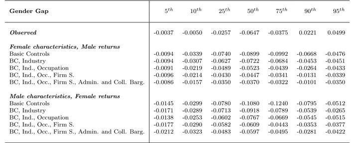
Table 4: Decomposition results
Gender Gap 5th 10th 25th 50th 75th 90th 95th
Observed -0.0037 -0.0050 -0.0257 -0.0647 -0.0375 0.0221 0.0499 Female characteristics, Male returns
Basic Controls -0.0094 -0.0339 -0.0740 -0.0899 -0.0992 -0.0668 -0.0476 BC, Industry -0.0094 -0.0307 -0.0627 -0.0722 -0.0684 -0.0453 -0.0451 BC, Ind., Occupation -0.0091 -0.0219 -0.0489 -0.0523 -0.0439 -0.0264 -0.0433 BC, Ind., Occ., Firm S. -0.0096 -0.0214 -0.0430 -0.0447 -0.0341 -0.0131 -0.0339 BC, Ind., Occ., Firm S., Admin. and Coll. Barg. -0.0086 -0.0157 -0.0350 -0.0370 -0.0322 -0.0101 -0.0350 Male characteristics, Female returns
Basic Controls -0.0145 -0.0299 -0.0780 -0.1080 -0.1240 -0.0795 -0.0512 BC, Industry -0.0171 -0.0289 -0.0713 -0.0918 -0.0789 -0.0539 -0.0265 BC, Ind., Occupation -0.0138 -0.0253 -0.0602 -0.0767 -0.0669 -0.0545 -0.0515 BC, Ind., Occ., Firm S. -0.0177 -0.0290 -0.0582 -0.0609 -0.0443 -0.0353 -0.0377 BC, Ind., Occ., Firm S., Admin. and Coll. Barg. -0.0212 -0.0323 -0.0483 -0.0597 -0.0495 -0.0281 -0.0422
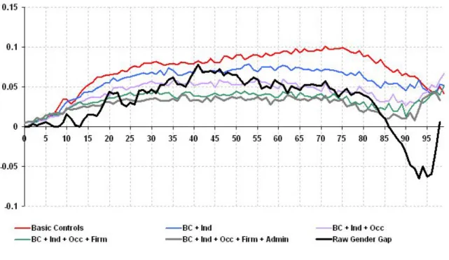
The results of the Machado-Mata decomposition are provided in Table 4 for specific quantiles. The first row in the table recites the raw gender wage gap. The first panel provides the gender gap calcu-lated using the counterfactual of male returns to female characteristics. The second panel provides the gender gap calculated using the counterfactual of female returns to male characteristics. The results are qualitatively similar. Figure 3 and Figure 4 present the same results for all percentiles. Figure 3 shows the gender gap at each quantile for various the counterfactuals constructed using male returns to female characteristics. It answers the following question: If males had female characteristics but were rewarded as they were males, what would the gender gap have been? Note that controlling for basic characteristics, such as education, age and tenure, widens the gender gap
considerably, especially at the top half of the distribution. At the median, the gender gap increases from 6.47 percent to 8.99 percent; at the 75th quantile, from 3.75 percent to 9.92 percent.
Observe again that the gender wage gap calculated at each percentile reveals a positive gap for the upper part of the wage distribution. In other words, raw data indicates that females have higher wages at the highest decile of the wage distribution. One of the most interesting results of the decomposition refers to this part of the distribution. When we construct a counterfactual wage distribution where female characteristics are being rewarded by male returns, we observe that the gender wage gap becomes negative at the top decile of the wage distribution as well. The gender wage gap at the ninetieth percentile changes from 4.99 percent to -4.76 percent, using only basic controls. In absolute value, this refers to a change of 10 percent.
Controlling for other characteristics such as industry, occupation and firm size, we can explain some part of the gender gap, especially between the 25th and 75th quantiles. The unexplained part of the gender gap shrinks from 7.8 percent to 4.83 percent on the 25th, and from 9.92 percent to 3.22 percent on the 75th quantile.
The reciprocal exercise provides results that move in similar directions. The question for Figure 4 is as follows: If females had male characteristics but were rewarded as females, what would the gender gap have been? Once again, controlling for basic characteristics widens the gender gap, however, adding controls for various firm-level characteristics explain smaller parts of the gender gap. When all controls are included, the gender gap does not seem to be much smaller than the observed gender gap. Moreover, it becomes considerably wider at the lower and at the upper part of the distribution.
To sum up, the decomposition results reveal that the gender gap in wages stem from differences in returns to labor market characteristics. If we assume that males had female characteristics, controlling for basic characteristics actually widens the gender gap, but including firm-level controls help explain some of it. On the other hand, if we assume that females had male characteristics, we find that the gender gap becomes much wider, and even when we include all controls, we fail to explain the observed gender gap.
7
Conclusion
In this paper, we study the gender wage gap along the wage distribution in Turkey, using a firm level data set. A couple of striking patterns emerge. The gender gap seems to be very close to zero at the lower end of the distribution. Moreover, at the higher end of the distribution, it looks as if women actually have higher wages than men.
Following the literature, we conduct quantile regressions to study the gender gap along the wage distribution. We start with a basic regression where we assume that the returns to labor market characteristics are the same for both genders. We find that controlling for education widens the gender gap considerably. Adding arguably endogenous variables such as industry, occupation and firm-level variables reduce the gender wage gap. The largest reduction happens around the median. On the other hand, we find that there is a sizeable gender gap that cannot be accounted for by differences in characteristics at the upper end of the wage distribution.
Figure 3: Machado-Mata Decomposition: Xfβm− Xfβf
Estimating separate quantile regressions for males and females, we find that the returns to labor market characteristics are different for males and females. Different returns for different genders indicate that the pooled regression results may provide a partial outlook on the gender gap. There-fore, we decompose the gender wage gap into a part stemming from differences in characteristics and a part from differences in returns. This decomposition exercise shows that at least half of the gender gap is due to differences in returns. We try to answer the following question: If males had female characteristics, what would the gender gap have been? Controlling for education, we find that the gender gap is actually much larger than what the raw data indicates. Including other con-trols, we can explain about half of the gender gap around the median, and even less at other parts of the distribution. The analogous question for males tries to document the counterfactual gender gap constructed from male characteristics being rewarded by female returns. This counterfactual gender gap is even larger. Controlling for education widens the gender gap and including other controls can only reduce it to the observed gender gap at best. In other words, the decomposition exercises indicate that the gender wage gap originates in large part from differences in returns. Even though the data set that we use allows us to study the industry and occupation as well as some other firm-level characteristics in detail, it does not provide any information on selection. Note that estimates of the gender wage gap may be biased by selection since wages are only observed for those who are selected into employment. This may potentially have important implications for the overall wage gap as the female employment rates are particularly low in Turkey. The female employment rate was 16.3 percent in 2006, whereas the male employment rate was 61.7 percent.7. Therefore, the results should be interpreted keeping this caveat in mind.
References
Albrecht, J., A. Bjorklund, and S. Vroman (2003, January). Is there a glass ceiling in sweden? Journal of Labor Economics 21 (1), 145–177.
Albrecht, J., A. van Vuuren, and S. Vroman (2009, August). Counterfactual distributions with sample selection adjustments: Econometric theory and an application to the netherlands. Labour Economics 16 (4), 383–396.
Amuedo-Dorantes, C. and S. de la Rica (2005). The impact of gender segregation on male-female wage differentials: Evidence from matched employer-employee data for Spain. IZA Discussion Papers 1742, Institute for the Study of Labor (IZA).
Antn, J. I., R. M. de Bustillo, and M. Carrera (2010, November). Labor market performance of latin american and caribbean immigrants in spain. Journal of Applied Economics 0, 233–261. Antonczyk, D., B. Fitzenberger, and K. Sommerfeld (2010, October). Rising wage inequality, the
decline of collective bargaining, and the gender wage gap. Labour Economics 17 (5), 835–847. Arulampalam, W., A. L. Booth, and M. L. Bryan (2007, January). Is there a glass ceiling over
europe? exploring the gender pay gap across the wage distribution. Industrial and Labor Relations Review 60 (2), 163–186.
Bayard, K., J. Hellerstein, D. Neumark, and K. Troske (2003). New evidence on sex segregation and sex differences in wages from matched employee-employer data. Journal of Labor Eco-nomics 21 (4), 887–922.
Blinder, A. S. (1973). Wage discrimination: Reduced form and structural estimates. The Journal of Human Resources 8 (4), 436–455.
Cudeville, E. and L. Y. Gurbuzer (2010). Gender wage discrimination in the turkish labor market: Can turkey be part of europe? Comparative Economic Studies 52 (3), 429–463.
Darbaz, B. and G. Uysal-Kolasin (2009). Collective bargaining in Turkey. Betam Research Brief 28, Bahcesehir University Center for Economic and Social Research(Betam).
Dayıo˘glu, M. and I. Tunalı (2004). Falling behind while catching up: Changes in the female-male wage differential in urban Turkey, 1988 to 1994.
Dayıoˇglu, M. and Z. Kasnakoˇglu (1997). Kentsel kesimde kadin ve erkeklerin isgucune katilimlari ve kazanc farkliliklari. Metu Studies in Development 24 (3), 329–361.
Groshen, E. L. (1991). The structure of the female/male wage differential: Is it who you are,what you do, or where you work? Journal of Human Resources 26 (3), 457–472.
Gunduz-Hosgor, A. and J. Smits (2008). Variation in labor market participation of married women in Turkey. Women’s Studies International Forum 31 (2), 104–117.
Ilkkaracan, I. and R. Selim (2007). The gender wage gap in the Turkish labor market. LABOUR: Review of Labour Economics and Industrial Relations 21 (2), 563–593.
Jellal, M., C. Nordman, and F.-C. Wolff (2008). Evidence on the glass ceiling effect in france using matched worker-firm data. Applied Economics 40 (24), 3233–3250.
Kara, O. (2006). Occupational gender wage discrimination in Turkey. Journal of Economic Stud-ies 33 (2), 130–143.
Kunze, A. (2000). The determination of wages and the gender wage gap: A survey. IZA Discussion Papers 193, Institute for the Study of Labor (IZA).
Le, A. and P. Miller (2010). Glass ceiling and double disadvantage effects: women in the us labour market. Applied Economics 42 (5), 603–613.
Machado, J. A. F. and J. Mata (2005). Counterfactual decomposition of changes in wage distribu-tions using quantile regression. Journal of Applied Econometrics 20 (4), 445–465.
Oaxaca, R. (1973). Male-female wage differentials in urban labor markets. International Economic Review 14 (3), 693–709.
Ozcan, Y. Z., K. Metin-Ozcan, and S. Ucdogruk (2003). Wage differences by gender, wage and self employment in urban Turkey: The case of Istanbul. Journal of Economic Cooperation 24 (1), 1–24.
Rica, S., J. Dolado, and V. Llorens (2008, July). Ceilings or floors? gender wage gaps by education in spain. Journal of Population Economics 21 (3), 751–776.
Tansel, A. (1998). Self employment wage employment choice and returns to education for urban men and women in Turkey. Working Papers 9804, Economic Research Forum.
Tansel, A. (2003). Wage earners, self employed and gender in the informal sector in Turkey. Working Papers 0102, Economic Research Forum.
Tansel, A. (2004). Public-private employment choice, wage differentials and gender in Turkey. IZA Discussion Papers 1262, Institute for the Study of Labor (IZA).
Tansel, A. (2005). Public-private employment choice, wage differentials, and gender in turkey. Economic Development and Cultural Change 53 (2), 453–77.
A
Quantile regressions by gender
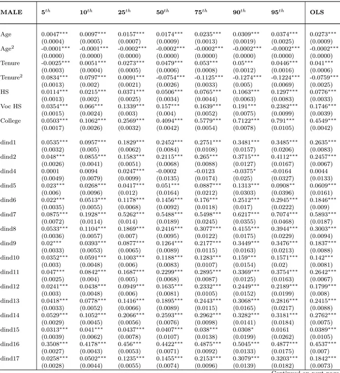
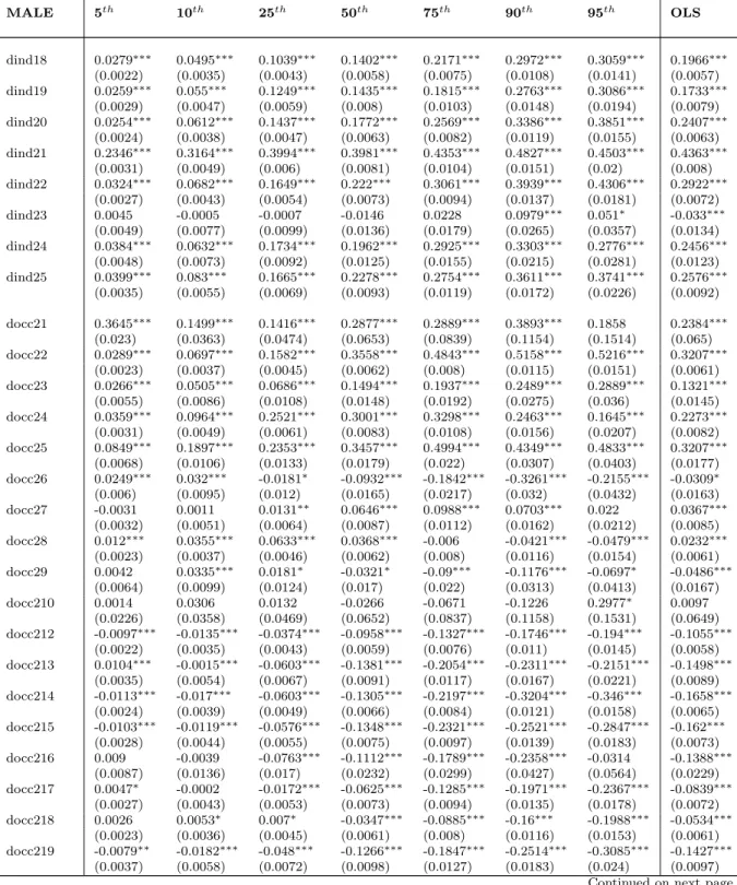
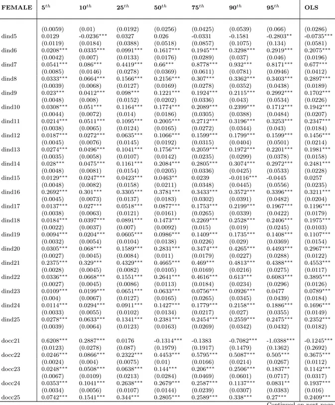
Table 5: Quantile Regressions by Gender(Basic Control, Industry, Occupation, Firm Size), MALE(n=141767)
MALE 5th 10th 25th 50th 75th 90th 95th OLS Age 0.0047∗∗∗ 0.0097∗∗∗ 0.0157∗∗∗ 0.0174∗∗∗ 0.0235∗∗∗ 0.0309∗∗∗ 0.0374∗∗∗ 0.0273∗∗∗ (0.0004) (0.0005) (0.0007) (0.0009) (0.0013) (0.0019) (0.0025) (0.0009) Age2 -0.0001∗∗∗ -0.0001∗∗∗ -0.0002∗∗∗ -0.0002∗∗∗ -0.0002∗∗∗ -0.0002∗∗∗ -0.0002∗∗∗ -0.0002∗∗∗ (0.0000) (0.0000) (0.0000) (0.0000) (0.0000) (0.0000) (0.0000) (0.0000) Tenure -0.0025∗∗∗ 0.0051∗∗∗ 0.0273∗∗∗ 0.0479∗∗∗ 0.053∗∗∗ 0.05∗∗∗ 0.0446∗∗∗ 0.041∗∗∗ (0.0003) (0.0004) (0.0005) (0.0006) (0.0008) (0.0012) (0.0016) (0.0006) Tenure2 0.0834∗∗∗ 0.0797∗∗∗ 0.0091∗∗∗ -0.0754∗∗∗ -0.1125∗∗∗ -0.1274∗∗∗ -0.1224∗∗∗ -0.0759∗∗∗ (0.0013) (0.002) (0.0021) (0.0026) (0.0033) (0.005) (0.0069) (0.0025) HS 0.0114∗∗∗ 0.0215∗∗∗ 0.0371∗∗∗ 0.0506∗∗∗ 0.0765∗∗∗ 0.1063∗∗∗ 0.1297∗∗∗ 0.0776∗∗∗ (0.0013) (0.002) (0.0025) (0.0034) (0.0044) (0.0063) (0.0083) (0.0033) Voc HS 0.0354∗∗∗ 0.066∗∗∗ 0.1339∗∗∗ 0.157∗∗∗ 0.1639∗∗∗ 0.191∗∗∗ 0.2382∗∗∗ 0.1746∗∗∗ (0.0015) (0.0024) (0.003) (0.004) (0.0052) (0.0075) (0.0099) (0.0039) College 0.0503∗∗∗ 0.1062∗∗∗ 0.2569∗∗∗ 0.4094∗∗∗ 0.5779∗∗∗ 0.7122∗∗∗ 0.791∗∗∗ 0.4549∗∗∗ (0.0017) (0.0026) (0.0032) (0.0042) (0.0054) (0.0078) (0.0105) (0.0042) dind1 0.0535∗∗∗ 0.0957∗∗∗ 0.1829∗∗∗ 0.2452∗∗∗ 0.2751∗∗∗ 0.3481∗∗∗ 0.3485∗∗∗ 0.2635∗∗∗ (0.0032) (0.005) (0.0062) (0.0084) (0.0108) (0.0157) (0.0206) (0.0083) dind2 0.048∗∗∗ 0.0855∗∗∗ 0.1583∗∗∗ 0.2115∗∗∗ 0.265∗∗∗ 0.3715∗∗∗ 0.4112∗∗∗ 0.2457∗∗∗ (0.0026) (0.0041) (0.0051) (0.0068) (0.0088) (0.0127) (0.0167) (0.0067) dind4 0.0001 0.0094 0.0247∗∗∗ -0.0002 -0.0123 -0.0375∗ -0.0164 0.0044 (0.0049) (0.0079) (0.0099) (0.0135) (0.0174) (0.025) (0.0327) (0.0133) dind5 0.023∗∗∗ 0.0268∗∗∗ 0.0417∗∗∗ 0.051∗∗∗ 0.0887∗∗∗ 0.1313∗∗∗ 0.0908∗∗ 0.0609∗∗∗ (0.006) (0.0096) (0.012) (0.0164) (0.0212) (0.0303) (0.0396) (0.0161) dind6 0.022∗∗∗ 0.0513∗∗∗ 0.1178∗∗∗ 0.1456∗∗∗ 0.176∗∗∗ 0.2512∗∗∗ 0.2945∗∗∗ 0.1846∗∗∗ (0.0035) (0.0055) (0.0068) (0.0092) (0.0118) (0.017) (0.0222) (0.009) dind7 0.0875∗∗∗ 0.1928∗∗∗ 0.5262∗∗∗ 0.5488∗∗∗ 0.5498∗∗∗ 0.6217∗∗∗ 0.7074∗∗∗ 0.5893∗∗∗ (0.0072) (0.0114) (0.014) (0.0189) (0.0245) (0.0355) (0.0468) (0.0187) dind8 0.0533∗∗∗ 0.1104∗∗∗ 0.1869∗∗∗ 0.2416∗∗∗ 0.3077∗∗∗ 0.4155∗∗∗ 0.3944∗∗∗ 0.3003∗∗∗ (0.0036) (0.0057) (0.007) (0.0095) (0.0122) (0.0175) (0.0229) (0.0094) dind9 0.02∗∗∗ 0.0393∗∗∗ 0.0877∗∗∗ 0.1264∗∗∗ 0.2177∗∗∗ 0.3449∗∗∗ 0.3476∗∗∗ 0.1837∗∗∗ (0.0033) (0.0053) (0.0065) (0.0089) (0.0115) (0.0163) (0.0213) (0.0088) dind10 0.0352∗∗∗ 0.0591∗∗∗ 0.1003∗∗∗ 0.1188∗∗∗ 0.1283∗∗∗ 0.159∗∗∗ 0.1571∗∗∗ 0.142∗∗∗ (0.003) (0.0048) (0.006) (0.0083) (0.0107) (0.0154) (0.02) (0.0081) dind11 0.047∗∗∗ 0.0842∗∗∗ 0.1687∗∗∗ 0.2299∗∗∗ 0.2895∗∗∗ 0.3369∗∗∗ 0.3754∗∗∗ 0.2642∗∗∗ (0.0025) (0.004) (0.005) (0.0068) (0.0087) (0.0125) (0.0163) (0.0067) dind12 0.0241∗∗∗ 0.0438∗∗∗ 0.0949∗∗∗ 0.1635∗∗∗ 0.2332∗∗∗ 0.2449∗∗∗ 0.2189∗∗∗ 0.1799∗∗∗ (0.003) (0.0048) (0.006) (0.0081) (0.0105) (0.0152) (0.0199) (0.008) dind13 0.0418∗∗∗ 0.0778∗∗∗ 0.1416∗∗∗ 0.1895∗∗∗ 0.2443∗∗∗ 0.3068∗∗∗ 0.2816∗∗∗ 0.2415∗∗∗ (0.0033) (0.0052) (0.0066) (0.0089) (0.0115) (0.0165) (0.0217) (0.0088) dind14 0.0529∗∗∗ 0.1052∗∗∗ 0.2066∗∗∗ 0.2593∗∗∗ 0.2962∗∗∗ 0.3282∗∗∗ 0.3181∗∗∗ 0.2762∗∗∗ (0.0029) (0.0045) (0.0056) (0.0076) (0.0098) (0.0141) (0.0184) (0.0075) dind15 0.0313∗∗∗ 0.041∗∗∗ 0.0437∗∗∗ 0.0407∗∗∗ 0.038∗∗∗ 0.0308∗ 0.0161 0.0389∗∗∗ (0.0039) (0.0062) (0.0078) (0.0107) (0.0138) (0.0199) (0.0262) (0.0105) dind16 0.3508∗∗∗ 0.4178∗∗∗ 0.456∗∗∗ 0.4422∗∗∗ 0.4875∗∗∗ 0.5045∗∗∗ 0.4877∗∗∗ 0.4537∗∗∗ (0.0027) (0.0043) (0.0053) (0.0071) (0.0092) (0.0133) (0.0175) (0.007) dind17 0.0258∗∗∗ 0.0502∗∗∗ 0.1235∗∗∗ 0.1455∗∗∗ 0.2153∗∗∗ 0.3079∗∗∗ 0.3203∗∗∗ 0.1842∗∗∗ (0.0028) (0.0044) (0.0055) (0.0074) (0.0096) (0.0139) (0.0182) (0.0073) Continued on next page
Table 5 – continued from previous page MALE 5th 10th 25th 50th 75th 90th 95th OLS dind18 0.0279∗∗∗ 0.0495∗∗∗ 0.1039∗∗∗ 0.1402∗∗∗ 0.2171∗∗∗ 0.2972∗∗∗ 0.3059∗∗∗ 0.1966∗∗∗ (0.0022) (0.0035) (0.0043) (0.0058) (0.0075) (0.0108) (0.0141) (0.0057) dind19 0.0259∗∗∗ 0.055∗∗∗ 0.1249∗∗∗ 0.1435∗∗∗ 0.1815∗∗∗ 0.2763∗∗∗ 0.3086∗∗∗ 0.1733∗∗∗ (0.0029) (0.0047) (0.0059) (0.008) (0.0103) (0.0148) (0.0194) (0.0079) dind20 0.0254∗∗∗ 0.0612∗∗∗ 0.1437∗∗∗ 0.1772∗∗∗ 0.2569∗∗∗ 0.3386∗∗∗ 0.3851∗∗∗ 0.2407∗∗∗ (0.0024) (0.0038) (0.0047) (0.0063) (0.0082) (0.0119) (0.0155) (0.0063) dind21 0.2346∗∗∗ 0.3164∗∗∗ 0.3994∗∗∗ 0.3981∗∗∗ 0.4353∗∗∗ 0.4827∗∗∗ 0.4503∗∗∗ 0.4363∗∗∗ (0.0031) (0.0049) (0.006) (0.0081) (0.0104) (0.0151) (0.02) (0.008) dind22 0.0324∗∗∗ 0.0682∗∗∗ 0.1649∗∗∗ 0.222∗∗∗ 0.3061∗∗∗ 0.3939∗∗∗ 0.4306∗∗∗ 0.2922∗∗∗ (0.0027) (0.0043) (0.0054) (0.0073) (0.0094) (0.0137) (0.0181) (0.0072) dind23 0.0045 -0.0005 -0.0007 -0.0146 0.0228 0.0979∗∗∗ 0.051∗ -0.033∗∗∗ (0.0049) (0.0077) (0.0099) (0.0136) (0.0179) (0.0265) (0.0357) (0.0134) dind24 0.0384∗∗∗ 0.0632∗∗∗ 0.1734∗∗∗ 0.1962∗∗∗ 0.2925∗∗∗ 0.3303∗∗∗ 0.2776∗∗∗ 0.2456∗∗∗ (0.0048) (0.0073) (0.0092) (0.0125) (0.0155) (0.0215) (0.0281) (0.0123) dind25 0.0399∗∗∗ 0.083∗∗∗ 0.1665∗∗∗ 0.2278∗∗∗ 0.2754∗∗∗ 0.3611∗∗∗ 0.3741∗∗∗ 0.2576∗∗∗ (0.0035) (0.0055) (0.0069) (0.0093) (0.0119) (0.0172) (0.0226) (0.0092) docc21 0.3645∗∗∗ 0.1499∗∗∗ 0.1416∗∗∗ 0.2877∗∗∗ 0.2889∗∗∗ 0.3893∗∗∗ 0.1858 0.2384∗∗∗ (0.023) (0.0363) (0.0474) (0.0653) (0.0839) (0.1154) (0.1514) (0.065) docc22 0.0289∗∗∗ 0.0697∗∗∗ 0.1582∗∗∗ 0.3558∗∗∗ 0.4843∗∗∗ 0.5158∗∗∗ 0.5216∗∗∗ 0.3207∗∗∗ (0.0023) (0.0037) (0.0045) (0.0062) (0.008) (0.0115) (0.0151) (0.0061) docc23 0.0266∗∗∗ 0.0505∗∗∗ 0.0686∗∗∗ 0.1494∗∗∗ 0.1937∗∗∗ 0.2489∗∗∗ 0.2889∗∗∗ 0.1321∗∗∗ (0.0055) (0.0086) (0.0108) (0.0148) (0.0192) (0.0275) (0.036) (0.0145) docc24 0.0359∗∗∗ 0.0964∗∗∗ 0.2521∗∗∗ 0.3001∗∗∗ 0.3298∗∗∗ 0.2463∗∗∗ 0.1645∗∗∗ 0.2273∗∗∗ (0.0031) (0.0049) (0.0061) (0.0083) (0.0108) (0.0156) (0.0207) (0.0082) docc25 0.0849∗∗∗ 0.1897∗∗∗ 0.2353∗∗∗ 0.3457∗∗∗ 0.4994∗∗∗ 0.4349∗∗∗ 0.4833∗∗∗ 0.3207∗∗∗ (0.0068) (0.0106) (0.0133) (0.0179) (0.022) (0.0307) (0.0403) (0.0177) docc26 0.0249∗∗∗ 0.032∗∗∗ -0.0181∗ -0.0932∗∗∗ -0.1842∗∗∗ -0.3261∗∗∗ -0.2155∗∗∗ -0.0309∗ (0.006) (0.0095) (0.012) (0.0165) (0.0217) (0.032) (0.0432) (0.0163) docc27 -0.0031 0.0011 0.0131∗∗ 0.0646∗∗∗ 0.0988∗∗∗ 0.0703∗∗∗ 0.022 0.0367∗∗∗ (0.0032) (0.0051) (0.0064) (0.0087) (0.0112) (0.0162) (0.0212) (0.0085) docc28 0.012∗∗∗ 0.0355∗∗∗ 0.0633∗∗∗ 0.0368∗∗∗ -0.006 -0.0421∗∗∗ -0.0479∗∗∗ 0.0232∗∗∗ (0.0023) (0.0037) (0.0046) (0.0062) (0.008) (0.0116) (0.0154) (0.0061) docc29 0.0042 0.0335∗∗∗ 0.0181∗ -0.0321∗ -0.09∗∗∗ -0.1176∗∗∗ -0.0697∗ -0.0486∗∗∗ (0.0064) (0.0099) (0.0124) (0.017) (0.022) (0.0313) (0.0413) (0.0167) docc210 0.0014 0.0306 0.0132 -0.0266 -0.0671 -0.1226 0.2977∗ 0.0097 (0.0226) (0.0358) (0.0469) (0.0652) (0.0837) (0.1158) (0.1531) (0.0649) docc212 -0.0097∗∗∗ -0.0135∗∗∗ -0.0374∗∗∗ -0.0958∗∗∗ -0.1327∗∗∗ -0.1746∗∗∗ -0.194∗∗∗ -0.1055∗∗∗ (0.0022) (0.0035) (0.0043) (0.0059) (0.0076) (0.011) (0.0145) (0.0058) docc213 0.0104∗∗∗ -0.0015∗∗∗ -0.0603∗∗∗ -0.1381∗∗∗ -0.2054∗∗∗ -0.2311∗∗∗ -0.2151∗∗∗ -0.1498∗∗∗ (0.0035) (0.0054) (0.0067) (0.0091) (0.0117) (0.0167) (0.0221) (0.0089) docc214 -0.0113∗∗∗ -0.017∗∗∗ -0.0603∗∗∗ -0.1305∗∗∗ -0.2197∗∗∗ -0.3204∗∗∗ -0.346∗∗∗ -0.1658∗∗∗ (0.0024) (0.0039) (0.0049) (0.0066) (0.0084) (0.0121) (0.0158) (0.0065) docc215 -0.0103∗∗∗ -0.0119∗∗∗ -0.0576∗∗∗ -0.1348∗∗∗ -0.2321∗∗∗ -0.2521∗∗∗ -0.2847∗∗∗ -0.162∗∗∗ (0.0028) (0.0044) (0.0055) (0.0075) (0.0097) (0.0139) (0.0183) (0.0073) docc216 0.009 -0.0039 -0.0763∗∗∗ -0.1112∗∗∗ -0.1789∗∗∗ -0.2358∗∗∗ -0.0314 -0.1388∗∗∗ (0.0087) (0.0136) (0.017) (0.0232) (0.0299) (0.0427) (0.0564) (0.0229) docc217 0.0047∗ -0.0002 -0.0172∗∗∗ -0.0625∗∗∗ -0.1285∗∗∗ -0.1971∗∗∗ -0.2367∗∗∗ -0.0839∗∗∗ (0.0027) (0.0043) (0.0053) (0.0073) (0.0094) (0.0135) (0.0178) (0.0072) docc218 0.0026 0.0053∗ 0.007∗ -0.0347∗∗∗ -0.0885∗∗∗ -0.16∗∗∗ -0.1988∗∗∗ -0.0534∗∗∗ (0.0023) (0.0036) (0.0045) (0.0061) (0.008) (0.0116) (0.0153) (0.0061) docc219 -0.0079∗∗ -0.0182∗∗∗ -0.048∗∗∗ -0.1266∗∗∗ -0.1847∗∗∗ -0.2514∗∗∗ -0.3085∗∗∗ -0.1427∗∗∗ (0.0037) (0.0058) (0.0072) (0.0098) (0.0127) (0.0183) (0.024) (0.0097) Continued on next page
Table 5 – continued from previous page MALE 5th 10th 25th 50th 75th 90th 95th OLS docc220 -0.004∗ -0.0109∗∗∗ -0.041∗∗∗ -0.1082∗∗∗ -0.1845∗∗∗ -0.2297∗∗∗ -0.2836∗∗∗ -0.1267∗∗∗ (0.0028) (0.0044) (0.0054) (0.0073) (0.0093) (0.0133) (0.0173) (0.0072) docc221 0.0105∗∗∗ 0.023∗∗∗ 0.0031 -0.0623∗∗∗ -0.1285∗∗∗ -0.2077∗∗∗ -0.2439∗∗∗ -0.0859∗∗∗ (0.0032) (0.005) (0.0062) (0.0084) (0.0109) (0.0157) (0.0208) (0.0083) docc222 -0.0004 -0.0083∗∗ -0.0356∗∗∗ -0.11∗∗∗ -0.1888∗∗∗ -0.2251∗∗∗ -0.2543∗∗∗ -0.1184∗∗∗ (0.0024) (0.0038) (0.0047) (0.0064) (0.0083) (0.0119) (0.0157) (0.0063) docc223 0.0004 0.0048 -0.0232∗∗∗ -0.0976∗∗∗ -0.1882∗∗∗ -0.2705∗∗∗ -0.3059∗∗∗ -0.1362∗∗∗ (0.0026) (0.004) (0.005) (0.0068) (0.0088) (0.0127) (0.0167) (0.0067) docc224 -0.0246∗∗∗ -0.0455∗∗∗ -0.111∗∗∗ -0.1888∗∗∗ -0.2996∗∗∗ -0.3836∗∗∗ -0.4249∗∗∗ -0.2361∗∗∗ (0.0025) (0.004) (0.0049) (0.0067) (0.0086) (0.0126) (0.0167) (0.0066) docc225 -0.029∗∗∗ -0.0449∗∗∗ -0.159∗∗∗ -0.2025∗∗∗ -0.1863∗∗∗ -0.3722∗∗∗ -0.4712∗∗∗ -0.2377∗∗∗ (0.0118) (0.019) (0.0238) (0.0324) (0.0419) (0.0599) (0.0773) (0.032) docc226 -0.0061∗∗∗ -0.0103∗∗∗ -0.0426∗∗∗ -0.1122∗∗∗ -0.1974∗∗∗ -0.2645∗∗∗ -0.2983∗∗∗ -0.1425∗∗∗ (0.0023) (0.0037) (0.0046) (0.0063) (0.0081) (0.0117) (0.0153) (0.0062) dfirmsize22 0.0177∗∗∗ 0.0413∗∗∗ 0.0772∗∗∗ 0.108∗∗∗ 0.1397∗∗∗ 0.1382∗∗∗ 0.1291∗∗∗ 0.1394∗∗∗ (0.0012) (0.0019) (0.0024) (0.0032) (0.0042) (0.006) (0.0079) (0.0032) dfirmsize23 0.0564∗∗∗ 0.1112∗∗∗ 0.2072∗∗∗ 0.2666∗∗∗ 0.278∗∗∗ 0.2693∗∗∗ 0.2482∗∗∗ 0.2823∗∗∗ (0.0013) (0.002) (0.0023) (0.003) (0.0038) (0.0056) (0.0074) (0.003) constant 6.1322∗∗∗ 5.9862∗∗∗ 5.8201∗∗∗ 5.8754∗∗∗ 5.9159∗∗∗ 5.962∗∗∗ 6.0015∗∗∗ 5.6694∗∗∗ (0.0068) (0.0104) (0.0131) (0.0183) (0.0245) (0.0367) (0.0493) (0.018) Standard errors in parentheses *** p<0.01, ** p<0.05, * p<0.1
Table 6: Quantile Regressions by Gender(Basic Control, Industry, Occupation, Firm Size), FEMALE(n=40298)
FEMALE 5th 10th 25th 50th 75th 90th 95th OLS age 0.0042∗∗∗ 0.0079∗∗∗ 0.0198∗∗∗ 0.0325∗∗∗ 0.0426∗∗∗ 0.0563∗∗∗ 0.0659∗∗∗ 0.0485∗∗∗ (0.0004) (0.0007) (0.0013) (0.0018) (0.0031) (0.0042) (0.0055) (0.002) age2 -0.0001∗∗∗ -0.0001∗∗∗ -0.0002∗∗∗ -0.0004∗∗∗ -0.0004∗∗∗ -0.0005∗∗∗ -0.0006∗∗∗ -0.0005∗∗∗ (0) (0) (0) (0) (0) (0.0001) (0.0001) (0) tenure -0.003∗∗∗ -0.0001∗∗∗ 0.02∗∗∗ 0.0372∗∗∗ 0.0478∗∗∗ 0.0434∗∗∗ 0.0408∗∗∗ 0.0362∗∗∗ (0.0004) (0.0006) (0.001) (0.0012) (0.0019) (0.0026) (0.0033) (0.0013) Tenure2 0.0752∗∗∗ 0.1042∗∗∗ 0.035∗∗∗ -0.0592∗∗∗ -0.1186∗∗∗ -0.1079∗∗∗ -0.0994∗∗∗ -0.0749∗∗∗ (0.0017) (0.0028) (0.0047) (0.0056) (0.0093) (0.0126) (0.0166) (0.0062) HS 0.01∗∗∗ 0.0221∗∗∗ 0.0443∗∗∗ 0.0944∗∗∗ 0.1318∗∗∗ 0.1633∗∗∗ 0.1682∗∗∗ 0.1229∗∗∗ (0.0017) (0.0029) (0.0055) (0.0072) (0.0119) (0.015) (0.0187) (0.008) Voc HS 0.0155∗∗∗ 0.031∗∗∗ 0.0774∗∗∗ 0.1602∗∗∗ 0.1868∗∗∗ 0.2063∗∗∗ 0.2084∗∗∗ 0.1765∗∗∗ (0.0023) (0.0037) (0.0071) (0.0094) (0.0154) (0.0197) (0.025) (0.0104) College 0.0301∗∗∗ 0.0675∗∗∗ 0.1899∗∗∗ 0.3671∗∗∗ 0.506∗∗∗ 0.6663∗∗∗ 0.7052∗∗∗ 0.4154∗∗∗ (0.002) (0.0033) (0.0062) (0.008) (0.0131) (0.0168) (0.0212) (0.0089) dind1 0.042∗∗∗ 0.073∗∗∗ 0.1901∗∗∗ 0.2263∗∗∗ 0.2327∗∗∗ 0.2587∗∗∗ 0.205∗∗∗ 0.2437∗∗∗ (0.0062) (0.0103) (0.0195) (0.0261) (0.0429) (0.0548) (0.0664) (0.0291) dind2 0.0194∗∗∗ 0.0464∗∗∗ 0.1173∗∗∗ 0.1589∗∗∗ 0.2404∗∗∗ 0.3076∗∗∗ 0.3237∗∗∗ 0.1975∗∗∗ (0.0032) (0.0054) (0.0101) (0.0133) (0.022) (0.0283) (0.0353) (0.0148) dind4 0.0095∗ 0.0086 -0.0068∗∗∗ 0.0121 -0.0172 -0.0181 -0.0101 -0.028∗∗∗
Table 6 – continued from previous page FEMALE 5th 10th 25th 50th 75th 90th 95th OLS (0.0059) (0.01) (0.0192) (0.0256) (0.0425) (0.0539) (0.066) (0.0286) dind5 0.0129 -0.0236∗∗∗ 0.0327 0.026 -0.0331 -0.1581 -0.2803∗∗ -0.0735∗∗∗ (0.0119) (0.0184) (0.0388) (0.0518) (0.0857) (0.1075) (0.134) (0.0581) dind6 0.0208∗∗∗ 0.0335∗∗∗ 0.0991∗∗∗ 0.1617∗∗∗ 0.1945∗∗∗ 0.3298∗∗∗ 0.2919∗∗∗ 0.2075∗∗∗ (0.0042) (0.007) (0.0133) (0.0176) (0.0289) (0.037) (0.046) (0.0196) dind7 0.0541∗∗∗ 0.086∗∗∗ 0.4419∗∗∗ 0.66∗∗∗ 0.8778∗∗∗ 0.932∗∗∗ 0.8171∗∗∗ 0.677∗∗∗ (0.0085) (0.0146) (0.0278) (0.0369) (0.0611) (0.0781) (0.0946) (0.0412) dind8 0.0333∗∗∗ 0.0664∗∗∗ 0.1566∗∗∗ 0.2156∗∗∗ 0.307∗∗∗ 0.3362∗∗∗ 0.3403∗∗∗ 0.2897∗∗∗ (0.0039) (0.0068) (0.0127) (0.0169) (0.0278) (0.0352) (0.0438) (0.0189) dind9 0.023∗∗∗ 0.0412∗∗∗ 0.098∗∗∗ 0.1221∗∗∗ 0.1924∗∗∗ 0.2115∗∗∗ 0.2992∗∗∗ 0.1702∗∗∗ (0.0048) (0.008) (0.0152) (0.0202) (0.0336) (0.043) (0.0534) (0.0226) dind10 0.0308∗∗∗ 0.051∗∗∗ 0.1164∗∗∗ 0.1774∗∗∗ 0.2089∗∗∗ 0.2399∗∗∗ 0.1712∗∗∗ 0.1942∗∗∗ (0.0044) (0.0072) (0.014) (0.0186) (0.0305) (0.0388) (0.0484) (0.0207) dind11 0.0214∗∗∗ 0.0511∗∗∗ 0.1095∗∗∗ 0.2005∗∗∗ 0.2712∗∗∗ 0.3196∗∗∗ 0.3253∗∗∗ 0.2347∗∗∗ (0.0038) (0.0065) (0.0124) (0.0165) (0.0272) (0.0344) (0.043) (0.0184) dind12 0.0187∗∗∗ 0.0272∗∗∗ 0.0635∗∗∗ 0.1066∗∗∗ 0.1599∗∗∗ 0.1799∗∗∗ 0.1599∗∗∗ 0.1456∗∗∗ (0.0045) (0.0076) (0.0145) (0.0192) (0.0315) (0.0404) (0.0501) (0.0214) dind13 0.0274∗∗∗ 0.0496∗∗∗ 0.1041∗∗∗ 0.1756∗∗∗ 0.2059∗∗∗ 0.1972∗∗∗ 0.2201∗∗∗ 0.1981∗∗∗ (0.0035) (0.0058) (0.0107) (0.0142) (0.0235) (0.0299) (0.0378) (0.0158) dind14 0.028∗∗∗ 0.0475∗∗∗ 0.1161∗∗∗ 0.2084∗∗∗ 0.2805∗∗∗ 0.3074∗∗∗ 0.2972∗∗∗ 0.2481∗∗∗ (0.0048) (0.0081) (0.0154) (0.0205) (0.0336) (0.0425) (0.0533) (0.0228) dind15 0.0129∗∗∗ 0.0247∗∗∗ 0.0423∗∗∗ 0.0463∗∗ 0.0239 -0.0116∗∗∗ -0.0445 0.0257 (0.0048) (0.0082) (0.0158) (0.0211) (0.0348) (0.0445) (0.0556) (0.0235) dind16 0.2692∗∗∗ 0.301∗∗∗ 0.3305∗∗∗ 0.3781∗∗∗ 0.3433∗∗∗ 0.3572∗∗∗ 0.3396∗∗∗ 0.3211∗∗∗ (0.0045) (0.0073) (0.0137) (0.0183) (0.0302) (0.0391) (0.0482) (0.0204) dind17 0.0137∗∗∗ 0.027∗∗∗ 0.0518∗∗∗ 0.0877∗∗∗ 0.1753∗∗∗ 0.2199∗∗∗ 0.1967∗∗∗ 0.1196∗∗∗ (0.0038) (0.0063) (0.0121) (0.0161) (0.0265) (0.0339) (0.0422) (0.0179) dind18 0.0184∗∗∗ 0.0397∗∗∗ 0.0891∗∗∗ 0.1473∗∗∗ 0.2269∗∗∗ 0.2528∗∗∗ 0.2406∗∗∗ 0.1975∗∗∗ (0.0022) (0.0037) (0.007) (0.0092) (0.015) (0.019) (0.0245) (0.0103) dind19 0.0094∗∗∗ 0.0204∗∗∗ 0.0605∗∗∗ 0.0986∗∗∗ 0.1409∗∗∗ 0.1735∗∗∗ 0.1408∗∗∗ 0.1107∗∗∗ (0.0032) (0.0054) (0.0104) (0.0138) (0.0226) (0.029) (0.0369) (0.0154) dind20 0.0305∗∗∗ 0.068∗∗∗ 0.1589∗∗∗ 0.2831∗∗∗ 0.3474∗∗∗ 0.4265∗∗∗ 0.4493∗∗∗ 0.2967∗∗∗ (0.0027) (0.0045) (0.0084) (0.011) (0.0179) (0.0227) (0.0288) (0.0122) dind21 0.2375∗∗∗ 0.329∗∗∗ 0.4329∗∗∗ 0.4665∗∗∗ 0.469∗∗∗ 0.4813∗∗∗ 0.4388∗∗∗ 0.4553∗∗∗ (0.0028) (0.0045) (0.0082) (0.0105) (0.0169) (0.0216) (0.0275) (0.0117) dind22 0.0336∗∗∗ 0.0668∗∗∗ 0.1551∗∗∗ 0.2641∗∗∗ 0.4616∗∗∗ 0.613∗∗∗ 0.6083∗∗∗ 0.3895∗∗∗ (0.0027) (0.0045) (0.0086) (0.0113) (0.0184) (0.0234) (0.0296) (0.0126) dind23 0.0109∗∗∗ 0.0199∗∗∗ 0.0651∗∗∗ 0.0633∗∗∗ 0.0756∗∗∗ 0.0926∗∗∗ 0.0477 0.0789∗∗∗ (0.004) (0.0067) (0.0127) (0.0165) (0.0265) (0.0345) (0.0439) (0.0184) dind24 0.0114∗∗∗ 0.0294∗∗∗ 0.0911∗∗∗ 0.1427∗∗∗ 0.1779∗∗∗ 0.2158∗∗∗ 0.1886∗∗∗ 0.1696∗∗∗ (0.0033) (0.0055) (0.0102) (0.0134) (0.0217) (0.027) (0.0355) (0.0149) dind25 0.0278∗∗∗ 0.0633∗∗∗ 0.1341∗∗∗ 0.2381∗∗∗ 0.2454∗∗∗ 0.2559∗∗∗ 0.2475∗∗∗ 0.2352∗∗∗ (0.0039) (0.0064) (0.0123) (0.0163) (0.0269) (0.0342) (0.0432) (0.0182) docc21 0.6208∗∗∗ 0.2887∗∗∗ 0.0176 -0.1314∗∗∗ -0.1383 -0.7082∗∗∗ -1.0388∗∗∗ -0.1245∗∗∗ (0.0123) (0.0278) (0.087) (0.1979) (0.1917) (0.1479) (0.1362) (0.2692) docc22 0.0246∗∗∗ 0.0866∗∗∗ 0.2322∗∗∗ 0.4453∗∗∗ 0.5795∗∗∗ 0.5087∗∗∗ 0.505∗∗∗ 0.3675∗∗∗ (0.0024) (0.004) (0.0075) (0.01) (0.0166) (0.0214) (0.0267) (0.0112) docc23 0.0248∗∗∗ 0.0508∗∗∗ 0.0638∗∗∗ 0.144∗∗∗ 0.206∗∗∗ 0.2506∗∗∗ 0.1837∗∗ 0.1142∗∗∗ (0.0067) (0.0109) (0.0213) (0.0284) (0.0469) (0.0601) (0.0717) (0.0317) docc24 0.0353∗∗∗ 0.1041∗∗∗ 0.2638∗∗∗ 0.2679∗∗∗ 0.2587∗∗∗ 0.1137∗∗∗ 0.0831∗∗ 0.1937∗∗∗ (0.0034) (0.0056) (0.0107) (0.0144) (0.0239) (0.0307) (0.0383) (0.016) docc25 0.0742∗∗∗ 0.1541∗∗∗ 0.344∗∗∗ 0.2805∗∗∗ 0.2589∗∗∗ 0.338∗∗∗ 0.27∗∗∗ 0.2409∗∗∗