Model predictive control: real-time issues and RBF-ANN implementation

Copyright©IFAC Automatic Systems for Building the Infrastructure

in Developing Countries, Istanbul, Republic of Turkey, 2003

ELSEVIER

IFAC

PUBLICATIONS

www.elsevier.com/JocaleJifac

MODEL PREDICTIVE CONTROL: REAL-TIME ISSUES AND RBF-ANN IMPLEMENTATION

IrenaI.Lokvenecl

*

and Georgi M. Dimirovski2

I University "Ss. Cyri! and Methodius ", Faculty ofElectrical Engineering

Institute ofAutomation& Systems Engg., MK-1000 Skopje, Rep. of Macedonia Fax# +389-48-416-201; Email: irena.lokvenec@mt.com.mk

*

Correspondence Author

2 Dogus University, Faculty ofEngineering, Department ofComputer Engg.

Acibadem - Kadikoy" TR-34722 Istanbul, Rep. of Turkey Fax# +90-216-327-9631; Emai!: gdimirovski@dogus.edu.tr

Abstract. Model predictive controls are control strategy in which the effect of the control actions are evaluated many steps in the future to gain an optimal control action. According to this the number of calculations made is very big and it needs some simplifications to use it in real time control tasks. That's why some recurrent formulas will be used. The GPC was realized with ANN using gradient descent algorithm which adjust the parameters of the ANN regulator withRBF.Copyright © 2003 1FAC

Keywords: ANN control, gradient, predictive control, predictor, regulator.

I. INTRODUCTION

Indirect learning predictive control schemes (Harris, 1995a) attempt to formulate a control strategy by assessing the effect of their action for many time-steps into the future and selecting the current optimal control action, which is then applied to the plant. The architecture requires the development of a plant model, a performance function to evaluate the effect of a control action (e.g. see Clarke et ai, 1987 a,b; Chen and Khalid, 1994). This is illustrated in Figure I, where a learning control element has also been included, so after sufficient training, the full optimization calculation does not need to be calculated and the computing resources can be used some ware else. Alternative control designs (Polycarpou, 1998 a, b; Jagannathan, 2001) with similar effect is to use

adaptive tracking by employing some kind of online neural network approximators.

In real time control tasks, however, many simplifications have to be incorporated into either of these designs in order to implement them. We have explored this line of research with regard to the indirect learning predictive control system architecture (e.g., Harris, 1995b; Lokvenec, 1996; Shilling, 2001; Saems, 1992;).

Adaptive predictive control (Clarke, 1991) indeed can be used in a great variety of problems. The results in closed-loop control are excellent should when the plant model is good. Multi-step ahead optimization calculation is expensive and time consuming. Moreover it can be successfully applied to systems which are not time-critical.

2. ON PREDICTIVE CONTROL 3. GPC IN A RBF-ANN IMPLEMENTATION _ _ _ .Q2.!mizati>nloop -)'I>(k+1;» ; yp(k+ 2) ANN pledickw

!

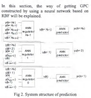
lU~l) ~ ANN _:regulalDn . 1 .

Fig 2. System structure of prediction Consider first that there is ANN predictor. Figure 2 shows the operating systemic structure of obtain the predictive controller obtained. Even though there several predictors shown in Figure 2, practically only one is used to do all the prediction as shall be seen in the sequel.

)1'(1<+Ii» --' - y(kHi>-l) -, y(i&'ti>...Y}----' ANN

I

u"'+ "'- ) ' regulak:> -I [ ,,:.: ..2 ! Hp-l I Uf<+ti>-pu)--j .

In this section, the way of getting GPC constructed by using a neural network based on RBF will be explained.

I

I

,--

~_:,h9

1 1 Outputof Objed T b j e c t 0esi1Dd output

Fig. 1. Control system architecture implementing the predictive control

u =

lu(k1u(k

+

11...,u(k

+

Hp

-l)j,

(1)

Yp=lvp(k+11""Yp(k+H p

)j,

(2)

Yr

=

lvr(k+11···,Yr(k+Hp)J.

(3)

Here Hp is a parameter which shows the size of the prediction horizon and Yp(k) is the output of the predictor in time k.

Let we have discrete time system with one input and one output. Let u(k) be the control signal at time k, yp(k) is the output of the process and y.(k) is the desired output. Vectors u, yp and Yrare:

In brief, the predictive controller is known to work this way: it generates that values of control u, so that the predicted output Yp is as closer as possible the desired output Yr' only fIrst value in the vector u is used to control the real process. This mode of control is known as principle of receding horizon. Next outputs of the process are generated by the model of the process. In that case it is called predictor.

To measure the quality of the control we use this function

Hp

J=~)Yp(k+i)-Yr(k+i)f.

(4)

i=1

The goal of the predictive control is to minimize the criteria J according of the control u. That means optimization of J by choosing optimal predictive control variable u.

General predictive control provides the basis for all types of predictive controls in general. Itcan be used in control of different problems: processes with not minimum phase, processes with death time, processes with unknown order, etc. Because of this, GPC concept can be used in construction of an ANN based controller implementation.

Let the process be described with the equation

y(k+ I)=J1y(k1...,y(k- PY+

1~u{k1

...,u(k - pu+ 1)]

(5) The simulation of the process will be than in the horizon of time

lk

+1,... ,k+

Hp

j.

I. At this moment k, ANN regulator number 0 will generate the control

u(

k )

which will be applied to the process and it will generate output

y(

k

+

1).

The control function of the regulator is

u(k)=!(Yr{k+Hpl""y,(k+l~y(k1 ,y(k - PY+l~ u(k -11 ,u(k - pu+

1»

(6)

In this case, regulator number 0 gives the control signal and the other regulators are used only for prediction.

2. In this step the prediction starts. Regulator number 1 will predict the control

u(k+I)=J(y,(k+Hpl""Y.(k+2h(k+I), ,y(k - PY+2}; u(k), ,u(k - pu+2)

This regulator has no need of

Y

r (

k

+

1).

The

control u(k+1) applied to the predictor gives Yp(k+

2).

3. Regulator number 2 gives u(k+2). It

uses Y_p(k+

2)

and u(k+

I)

which are predicted from the previous predictor

the gradient descent algorithm is used. Let

J.1._j

=

cons!

=

J.1..

If Lagrange formula is used, then according the functional constrains of the process

F

k+1

=

F(y(k1 ...,y(k- py+ 1},u(k1 ...,u(k- pu+ 1)]

(10) we obtain

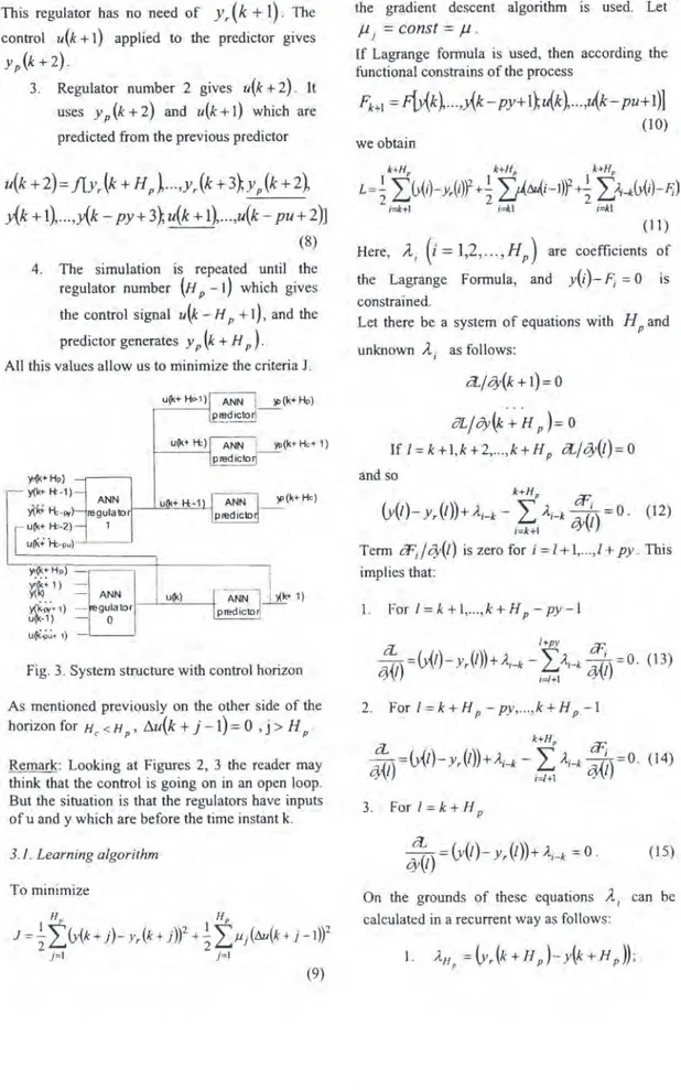
Fig.3.System structure with control horizon

u(k+Hp-') ANN

i

\I>(k+Hp)

p~cJ..i.~~-.':!-u(k

+

2)=

flYr (k

+

Hp

h...

,Yr (k

+

3},Y

p

(k

+

2~

y(k

+

1), ...,y(k - PY+ 3},u(k

+

1),...,u(k - pu

+

2)]

(8)

a-

/+py iF

:>1)

=

(y(l)- Yr(/))

+

A

i-k -

L

Iti-k

~/) =

O. (13)

'-Y\l i=/+1 '-Y\I

1. Forl=k+I, ...,k+Hp-Py-1

k+Hp k+Hp k+Hp

L=~ LG{i)-yAi)f+~ ll<~i-I)f+~

LA;-/cG{i)-F;)

1=k+1 l=kl l=kl

(11 ) Here,

AI

(i

=

1,2, ... ,H

p) are coefficients of

the Lagrange Formula, and

Y(i)-

F;

=0 is

constrained.

Let there be a system of equations with

Hp

and unknown

A

I as follows: cL/0'(k+

1)= 0

OL/t3y(k+Hp

)=

0 If_{l=k+I,k+2, ... ,k+H p cL/0'(I)=O} and so k+Hp iF.

(y(t)-Yr(t))+A

i-k -

LA

i-k

(~)=o.

(12) i=k+l

0'

Term iF,/0'(1) is zero for i=1+ 1,...,1+Py.This implies that:

lI'(k+ He)

--ANN--l~+ 1)

predictor.

4. The simulation is repeated until the

regulator number (Hp-I) which gives

the control signal u(k - Hp+

1),

and the predictor generates Yp(k+Hp). All this values allow us to minimize the criteriaJ.

~+Hp) ~-~

l-,,-

y'(f<;1-\,.",

"~')

regulatoJ----'-"""---''-'.:-'-!..j

A"'

[

~~~~~)n

1.__- - - - ,

y~~Hp)__m._____ !

r.;(k+1)

=

i

"I<) ANN i u(k)

y(~+ 1) - gulalor

u(k-1) - 0

U{l<~~+1)

-As mentioned previously on the other side of the horizon for Hc<H_p' ~u(k+j-l)=O

,j>H

_p'

Remark: Looking at Figures 2, 3 the reader may

think that the control is going on in an open loop. But the situation is that the regulators have inputs ofu and y which are before the time instant k.

2. Forl=k+H_p-Py,... ,k+H_p-1 3. For 1= k+Hp 3.1. Learning algorithm (15) To minimize Hp Hp J=

~

LG{k

+

j)-

Yr(k

+

j))2

+~

L,uj(fui(k

+

j _1))2

j=1 j=1 (9)

On the grounds of these equations

A

I can be

n

Yp(k'+I)= LWj9Sj(x), (16) j=\

Signals

y(

k

+

j)

can be replaced with

y

p

(k

+

j),

which are known, and only tF;+k /4'(k+j) has to be calculated. Thus let

where

Itmay well be found that the input vector is: XI =y(k'),

Xpy+1 =u(k'), x2 =y(k'

-I),

x py+2 =u(k'-I),

(23)

Xpy,R =y(k+R- py+

1)

Xpy+pu,R =u(k+R-pu+i)

X py+pu+Hp-R,R=Yr(k+R+

1).

...

,

Adaptation of the weights is computed by mean of

n

u(k+R)= LWJ,R9SJ(X), (21)

J=I

9S_J(X)=ex

J

_.!.

f

(Xi,R

~

Ci'J'Rf]. (22)

1

2 i=1 L.i,J,R

In here, WJ,R' Ci,J,R' I.i,J,R are the parameters of the RBF of the R-th regulator. Following the analysis presented above in this section, the input vector of the regulator R is found to be:

XI,R =y(k+R), X py+I,R

=

u(k+R), X py+pu+l,R=Yr(k+Hp),

X 2,R =y(k+ R-l), X py+2,R =u(k+R

-I)

X py+pu+2,R =Yr(k +H p

~I),

with

Let the ANN regulator

3.2. Gradient descent algorithm

(18) (17)

Xpy

=

y(k' - py+

I),

x py+pu =u(k' - pu+

I),

...

, ( I

~(x.-cf]

9S;(x)=exp - -

LJ

I 2',J . 2i=\ ai,j Hp tF Aj=(yr(k+j)-y(k+ j))+-

L~ ~j

i+lc .)'

i=l+1 0'\k+ }

j =Hp-I,Hp - 2,...,Hp - PY ;

j+py tF Aj

=

(YAk+j)- y(k+ j))+-

L~ ~j

i+lc .)'

i=I+1 0'\k+} j

=

Hp - Py-I,H p - Py-2, ...,I;

3.

2.

wherek'is

k+l,k+2, ... ,k+H

_p

-I.

Let, in addition, tF;+k /4'(k+j) be written in the

iF

form k+\+a. apparently for k'

=

k+a we

4'(k +b)' tF have K + I . q.{k'+b-a) where WJ,R(k+I)=WJ,R(k)-1J:- ' J,R CL _ CL ~(k+R)

OWJ,R - &(k+R) iWj,R .

(24 a)

(24 b)

and, because X_a-b+1=y(k'+b - a),we have

iFk+\+a '"

~w""\-

(Ca-b+I,J -Xa-b+l) (iO)

(

)

LJ

J'f'J 2 .

4' k+b J=\ a a-b+I,J

(25b) Should Fk'+I:::::: yp(k'+I)be valid, then

iFk'+1

4'

p(k'+

I)

4'(k'+b - a) '" 4'(k'+b -

a) ,

(19)

Adaptation of the centers is computed by means of

C_I,J,-R(k+I)=C_I,J,

"R(k)-l1~,

_'/it.' (25 a)

i,J,R

where

CL _ CL ~(k+R)

it.'- "R -_I,J, ~(k+R) it.'·R ._I,J,

Finally adaptation of the distances are computed by means of

where

Cl., Cl.,

m(k+R)

i2: ._I,j,R =

m(k

+

R)

i2:._I,j,R

And this concludes the design derived.

(27 b)

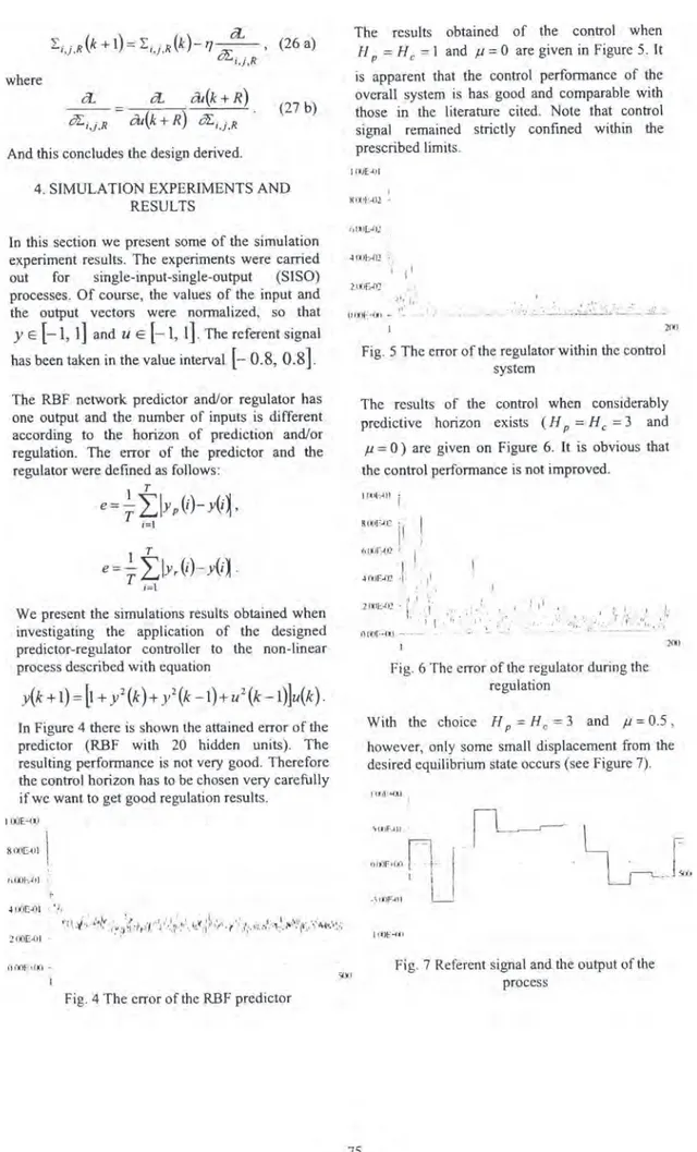
The results obtained of the control when Hp

=

He

=

1 and f.J

=

0 are given in Figure 5. It is apparent that the control perfonnance of the overall system is has good and comparable with those in the literature cited. Note that control signal remained strictly confined within the prescribed limits.

I uJE...fJI

4. SIMULATION EXPERIMENTS AND RESULTS I HI,(jf:..02 -21XJ ~":<iI OOO"'>(~1 _.ll~ .":'~_'• . _ .• : __ " . ' __.~.. ·~:·>.:..•.:•.•..:.:-•.:'_:,,:·.:. ..~~:~·{_:":"'':'''':'~L':':''' mlrAl] :, I !I

Fig. 5 The error of the regulator within the control system

~,'. 2.I~r;Al]

In this section we present some of the simulation experiment results. The experiments were carried out for single-input-single-output (SI SO) processes. Of course, the values of the input and the output vectors were nonnalized, so that

y E

[-1, 1]

and U E [-

1, 1].

The referent signal has been taken in the value interval [-

0.8, 0.8].

'"ll"AlI i

The results of the control when considerably predictive horizon exists (Hp = He =3 and f.J=0) are given on Figure 6. It is obvious that the control perfonnance is not improved.

201l

,;

' I I

• h . ''" ,";- :.\'l,~.

- . .,. --- j:"-~---~-':'

Fig. 6 The error of the regulator during the regulation glKiE·m

h

I 6tXiF·07: ~ 1 T e=-

IlyJi)-y(i).

T ;=1

We present the simulations results obtained when investigating the application of the designed predictor-regulator controller to the non-linear process described with equation

The RBF network predictor and/or regulator has one output and the number of inputs is different according to the horizon of prediction and/or regulation. The error of the predictor and the regulator were defined as follows:

1 T

e=-

IIYp(i)-y(i~,

T ;=\

In Figure 4 there is shown the attained error of the predictor (RBF with 20 hidden units). The resulting perfonnance is not very good. Therefore the control horizon has to be chosen very carefully if we want to get good regulation results.

With the choice Hp =He =3 and f.J=0.5, however, only some small displacement from the desired equilibrium state occurs (see Figure 7).

IU.ll'+O.l ,O:IE"{~I 8.lX'E'.l!

I

i 6.1~')E·OI : H'>!'4l1 __

~ ~_

""If";>

n-

I I

1

1

_1

r=

SIX,

.~I.)F-411

U

Fig. 4 The error of the RBF predictor

Fig. 7 Referent signal and the output of the process

This situation happens because the regulator has to fulfill two extremely different objectives:

(a) to follow the output of the process as closely as possible; and

(b) to limit the variation in the control signal. Hence the regulator has to make some balanced compromise between these two contradicting objectives. This is why no precise equilibrium can be attained, as depicted in Figure 7. However, this discrepancy is rather small and remains constant during the entire operation of the system.

5. CONCLUSION

Model predictive control is practically a rather desirable control concept, but it implies many calculations in order to select optimal control actions. Because of this intrinsic feature it is practically impossible to be used in real-time control of dynamical processes without some simplifications. In this paper a RBF artificial neural-network design has been proposed to cope with this issue for single-input-single-output (SISO) process control. The obvious future research is to investigate the multi-input-multi-output (MIMO) case albeit it seems to be a rather challenging task.

The recurrent formulas based on employing RBF neural networks, which were explained in Section 3, have some inputs that need to be calculated only once and than can be used in other steps. This reduces the number of calculations and makes MPC employing RBF ANN more amenable to real-time applications albeit the tracking may have some small off-set. Simulation experiments have confirmed reduction of computation time by a factor more than ten, while the control performance is only slightly improved.

It is therefore believed that the proposed design may well be a competitive alternative for non-linear process control.

REFERENCES

Brown, M. and C. J. Hams, (1994), Neural Networks for Modeling and Control - A Review. In:Advances in Intelligent Control, pp 17-56. World Scientific, Singapore.

Chen, F-C. and H. K. Khalid, (1994), Adaptive Control of Nonlinear Systems. In: Advances of Intelligent Control, pp 163-182. World Scientific, Singapore.

Clarke,D.W., C. Mathadi and P. S. Tuffs, (1987), "Generalized predictive control - PartI. The

basic algorithm."Automatica, vol. 23, no. 2, pp 137-148.

Clarke, D. W., C. Mathadi and P. S. Tuffs, (1987), "Generalized predictive control - Part

n.

extensions and interpretations." Automatica, vol. 23, no. 2, pp 149-160.

Clarke, D. W. (1991), Adaptive Generalized Predictive Control. In: Proceedings of the 4-th International Conference on Chemical Process Control CPCIV, Y. Arkun and W. H. Ray (eels.), South Padre Island,TX, pp. 395-417. Ge, S. S., C. C. Hang, T. H. Lee, and T. Zhang

(2002), Stable Adaptive Neural Network Control. Kluwer, Boston.

Hams, C. J., (1995a), Advances and Critical Research Issues in Intelligent Mode1ing, Control and Estimation. In:Proceedings of the First ESF-COSY Workshop on Control of Complex Systems, M. Thoma and R. Patton (eds.), Universita "La Sapienza", Rome. Hams, C. 1., (1995b), Instantaneous Learning

Algorithms. In: Advances of Intelligent Control, pp 158-217. World Scientific, Singapore.

Ivanoska (Lokvenec), I. I. (1996), Simulation Modeling and Self-Learning Control of Processes with Improved ANN (MSc. Thesis). SS Cyril and Methodius University, Skopje (in Macedonian).

Jagannathan, S. (2001), "Control of a class of discrete-time systems using multilayer neural networks."IEEE Trans. Neural Networks, vol. 12, no. 5, pp. 1113-1120.

Morari, M. (1993), Some Control Problems in the Process Industries. In: Essays in Control: Perspectives in the Theory and Its Applications (H. L. Trentelmann and J. C. Willems, eds.), pp. 55-77. Birkhaeser, Boston Basel Berlin. Polycarpou, M. M. (1998a), On-line

Approximators for Nonlinear System Identification: A Unified Approach. In: Neural Network Systems Techniques Applications (X.

Lenodes, ed.), vol. 7, pp. 127-155. The IEEE, Piscataway, N.J.

Polycarpou, M. M. (199S), "Stable adaptive tracking of uncertain systems using nonlinearly parameterized online approximators." Int. J. Control, vol. 70, no. 3, pp. 363-384.

Saerens, M. (1992), Approche Connexionniste de la Processus (These de doctorat), Universite Libre de Bruxelles, Bruxelles, Belgique (in French).

Shilling,R., J. J. Carroll, Jr., and A. F. AI-Ajlouni (2001), "Approximation of non linear systems with radial basis neural networks."IEEE Trans. Neural Networks, vol. 12, no. 1, pp. 1-15.