BATCH ORDERING INVENTORY MANAGEMENT UNDER THE MIXED DEMAND INFORMATION: A CASE STUDY
1Muzaffer ALIM , 2Patrick BEULLENS
1Batman Üniversitesi, Teknoloji Fakültesi, Otomotiv Mühendisliği Bölümü, Batman, TÜRKİYE 2Mathematical Sciences and Southampton Business School and CORMSIS, University of Southampton, UK
1 [email protected], 2[email protected]
(Geliş/Received: 31.07.2019; Kabul/Accepted in Revised Form: 25.04.2020)
ABSTRACT: This study is concerned with analysing the past demand data and development of an inventory model with demand arising from deterministic which is known in advance and random sources simultaneously. Two different shortages are created for each demand type and in order to prevent model to backlog the deterministic demand, very high shortage cost is given for deterministic demand. The numerical value of the parameters are obtained from a real case which the inventory system of an information and technological organization of a university. The main difference of this study from the previous studies is that the order amount must be in palette quantity for a deterministic and stochastic demand inventory problem. Under this constraint, an inventory model is developed and tested with several datasets. Assuming lead time as constant, the value of deterministic demand present in the system and impact of palette constraint are investigated. These investigations are compared with the status quo in the case study. It has seen that the palette quantity behaves as safety stock for high level random demand. Recommendations based on the impacts of advance demand information, lead time and pallet quantity are presented in terms of changing in ordering costs, holding costs and service level.
Key Words: Inventory model, batch ordering, deterministic and stochastic demand, mix integer programming
Karışık Talep Bilgisi Kapsamında Toplu Sipariş Envanter Yönetimi: Bir Durum Çalışması ÖZ: Bu çalışma, geçmiş dönem talep bilgisinin ve önceden bilinen deterministik ve rassal talep bilgisinin birlikte bulunduğu stok sistemlerinin analizini konu almaktadır. Herbir talep bilgisi için iki farklı talebi karşılayamama maliyeti belirlenmiş olup deterministik talebe verilen yüksek talep karşılayamama maliyeti bu tip talebin zamanında karşılanmamasını oldukça güç hale getirmektedir. Kullanılan veriler bir üniversitenin bilgi teknolojilerinden sorumlu olan birimden alınmıştır. Bu çalışmanın literatürdeki diğer çalışmalardan farkı aynı anda hem deterministik hem de rassal talep altında sipariş miktarının palet cinsinden olmasıdır. Bu kısıt altında, bir stok modeli geliştirilmiş ve farklı veriler altında sayısal olarak test edilmiştir. Sabit tedarik süresi varsayımı altında, deterministik talebin değeri ve paletle sipariş kısıtının etkileri ölçülmüştür. Bu ölçümler, mevcut durumla kıyaslanmıştır. Paletin içerik miktarının yüksek seviyedeki rassal talep için güvenli stok olarak davrandığı gözlemlenmiştir. Değişen sipariş maliyeti, stok tutma maliyeti ve hizmet seviyeleri altında ön talep bilgisi, tedarik süresi ve palet miktarının etkileri üzerine önerilerde bulunulmuştur.
1. INTRODUCTION
In many competitive business environments, inventory management plays an important role in managing the trade-off between maximising the service level of customers while minimising the operational costs. In order to meet the customer demands within a reasonable time, most businesses need to keep some amount in stock since the time it takes to order products from suppliers or produce the products from raw materials is too long in comparison. Another factor that leads to keep stock is that ordering or producing products efficiently often involves batches of (identical) products which are much larger that individual customer orders. Inventory management is defined as the control of amounts of products kept in stock over time. The principle purpose of inventory management is to answer the following two questions:
1. When do we need to place an order (or produce) for a given type of product? 2. How much of this product should we order?
Inventory management can lead to better results if the future demand is known. In real life at least some part of the future demand is not known with certainty beforehand, but needs to be estimated. Forecasting methods are required in order to avoid unwelcome surprises. According to Bon and Leng (2009), forecasting product demand is one of the most important issues in inventory management in both short and long term planning activities. The most appropriate forecasting method is to be chosen based on a good insight into what drives future demand. Observing seasonal patterns and trends from past data can be very helpful in certain situations, but may still lead to disastrous results if the assumption that the future is going to be very similar to the past does not hold. It may sometimes be more useful to investigate the processes that customers use to place their orders.
During the decision process in inventory management, costs and lead times are typically important considerations. Lead time is the time needed between placing the order at the supplier (or manufacturing floor) and the time the products requested become fully functionally available in the warehouse to meet customer demand. The relevant costs in an inventory model most often include the following four terms: holding cost, ordering cost, unit product cost and unit shortage cost. The shortage cost occurs when a demand does not met on time which the demand is called backorder. In this study, we have such a situation of backorders. It is still one of the difficult problems in inventory management theory to arrive at accurate estimates for the shortage cost. One way around this problem is to use an estimated value for this cost, and then to observe the service level achieved in the inventory model. If this service level achieved is too low, one can iterate by increasing this shortage cost until the service level has achieved a desirable level.
How to measure the service level is very dependent on the context. A simple measure is to count the number of orders delivered by the requested due date of the customer per unit of time (say in one month) and divide this number by the total number of orders delivered. A variation to this is to measure to count the total number of units of products that are delivered by the due date divided by the total number of units delivered. More refined measures of service level will also look at the lateness (the length of time between the due date and the actual delivery date) of orders.
Due to significant period-to-period or even day-to-day changes in demand levels, seasonality effects, trends, and constrained storage space, inventory management is a challenging task at the university’s IT department, but also critical for delivering a good service to the university. In the current situation, the inventory is controlled by the providence of staff and none of the economical trade-off analysis is being considered in the day-to-day decision making on the inventory. The main concern of the planners at the present is to be able to meet demand. Some automation is already in place to capture customer requests and keep a status of inventory records. The issues of when and how much to order from the suppliers, however, is still a decision unsupported by a computerised decision aiding model.
In this study, past demand data is going to be analysed to observe the demand pattern. This is complemented by an analysis of the potential difference in customer types as to investigation of the potential value of demand classification. It is then complemented by an analysis of the supply side by investigating the conditions under which the company can order from suppliers. Finally, we will
investigate the internal processes undertaken to prepare a product for release to the customer. A set of alternative inventory models is then to be developed and its performance evaluated under different demand profiles as well as compared with the real situation in terms of both service level and costs. Since the IT department delivers many products, this study will have to focus on a specific branch of products only: the high-value and high-volume standard computers/laptops series.
2. LITERATURE REVIEW
This study is mainly related to the fields of inventory management with deterministic and stochastic demand and batch ordering. Thus, we review the literature for demand management and order restrictions in inventory management.
According to Waters (1992), for the inventory control models, future demand is the most important input and has the biggest impact on stocks held. Therefore demand management is considered as the first step of inventory management. The complexity of the inventory model depends on the demand pattern as put by Taha (2007) and mainly the demand can be classified into deterministic demand which can be constant or variable over time and stochastic which can be stationary or non-stationary over time. Although the inventory model for the first type of demand is the simplest model (classic EOQ model), it has seen in practice not so often. On the other hand, the inventory models are able to deal with the fourth demand type are the most complex although this demand pattern is often likely to occur in real life. In the inventory literature, demand is assumed as deterministic or stochastic (for detailed review see Aloulou et al. (2013), Bushuev et al. (2015)). There is also a different type which assuming demand as advance demand at which some parts of the demand is known in advance but some part still remains uncertain (Gallego and Özer (2001), Sobel and Zhang (2001)).
Demand is placed in advance of their due dates are called as advance demand information. If customer lead time is less than the supply lead time, this type of demand must be satisfied by using on hand inventory and that’s why it can be classified as stochastic demand. Unlike the classical inventory models treated demand as either deterministic or stochastic, Sobel and Zhang (2001) consider the demand which arrives from a deterministic and stochastic source simultaneously. They mentioned that if deterministic and stochastic demands are considered separately, deterministic demands will not be backordered. However, this will bring higher holding and ordering costs due to keep inventory for both demands separately. Thus, they consider this two types of demand simultaneously. In their study, they consider periodic review inventory systems with demand priority. Deterministic demand is assumed to have non shortages whereas stochastic demand can be backlogged. This demand type is closely related to our problem case. However they assume that if there is stock on hand, the backorders must be satisfied even without considering for future period deterministic demand. However in our case, there must be a possibility of having positive inventory level while having some shortages. This is a result of having two different shortages costs for deterministic and stochastic demand separately. They proved that modified (s, S) policy is optimal for their case.
Similar to Sobel and Zhang (2001), Gallego and Özer (2001) studied the inventory management with advance demand information. They stated that customers have different willingness to pay for the speed of fulfilment of their order. They used dynamic programming (Bellman Equation) to find reorder level and order up to level. One of the interesting result in their study is to prove that for the cases with zero ordering/setup cost, the demand information beyond lead time has no operational value. Özer and Wei (2004) takes this study to an inventory problem with limited storage capacity and advance demand information. They measure the impact of advance demand information on capacitated inventory problem with advance demand. Wang and Toktay (2008) extend these studies by considering flexible delivery options without having a storage capacity. In contrast to the literature, they assumed that customers who placed their order for a due data can accept early delivery. They used some heuristics methods to find a way to making decisions. As a result of their study, they indicate that advance demand information is a powerful tool in reducing inventory costs. Numerical studies mention flexible delivery can contribute significant benefits to the solution.
Beside the demand side, there might also be some restrictions and uncertainties on supply side. One of these restrictions is minimum order quantity which the firm needs to order more than a minimum threshold amount (Kesen et al., 2010). This might be soft which can be relaxed with additional cost or be solid which cannot be relaxed. Another order restriction is batch ordering which allows orders only to be an integer number of a base quantity. Veinott (1965) is one of the first study consider batch ordering in inventory problem. Chen and Zheng (1994) considers the (r, nQ) policies for batch ordering inventory problems and Chen (2000) proves the optimality of (r, nQ) policy. Extention of the problem with lost sales has been considered by Van Woensel (2013). The multiechelon cases of batch ordering has been studied by Chao and Zhou (2009) and Shang and Zhou (2010).
3. PROBLEM DEFINITION
The academic staff and postgraduate students are allowed to request a computer from the university and the university kept stock to satisfy these request within a reasonable time. Some of these requests are placed in advance of the required date. Yet still some of the demand can be known at last minute. The university replenishes its stock from an external company and the company only allows the university to place its order in terms of pallets. The university aims to satisfy all demand within a threshold service time but due to having longer lead time than the service time, they need an effective inventory policy and they need to know the impact of batch ordering so that they can negotiate with the company. In this section, we provide the notation and mathematical formulation to be used to formulate the problem.
3.1. Notation
The variables and parameters used in the formulations are presented in this part. The mathematical model is constructed with the following notation.
𝐷𝑡 Deterministic demand in period t 𝑅𝑡 Random demand for period t 𝐸𝑡 Expected demand in period t
𝐼𝑡 On hand inventory at the end of period t 𝑦𝑡 Number of pallets ordered in period t 𝑧𝑡 𝐸xpected amount to be delivered in period t
𝐵(𝐷)𝑡 Number of backorders for deterministic demand in period t 𝐵(𝑅)𝑡 Number of backorders for random demand in period t 𝑋𝑡= { 1 𝑖𝑓 𝑎𝑛 𝑜𝑟𝑑𝑒𝑟 𝑝𝑙𝑎𝑐𝑒𝑑 𝑖𝑛 𝑝𝑒𝑟𝑖𝑜𝑑 𝑡
0 𝑜𝑡ℎ𝑒𝑟𝑤𝑖𝑠𝑒 𝑁 Planning Horizon (days)
𝐿 Lead time (days) ℎ Holding cost ( £
unit∗day) 𝑐 Ordering cost (order£ )
𝛽𝐷 Shortage cost for deterministic demand ( £ unit ∗ day) 𝛽𝑅 Shortage cost for random demand (
£ unit ∗ day) 𝑄 Number of computers in a pallette
3.2. Mathematical Formulation
The mathematical formulation of the inventory model with deterministic and stochastic demand and batch ordering is presented. The deterministic demand is known in advance of N days, (𝑁 ≥ 3), whereas stochastic demand is known in advance of 3 days only. At the beginning of period t, deterministic demand over {t, ..., t+N-1} and random demand over {t, ....,t+2} are known. The optimal inventory decisions are made by the on hand information and the decisions are applied for only at the current period. Then, at the end of the period with the new demand information, the demand is updated and the model is run for next N period. The rolling planning horizon approach is applied until reaching the expected time horizon. 𝑀𝑖𝑛 ℎ ∑𝑁𝑡=1𝐼𝑡 + 𝑐 ∑𝑁𝑡=1𝑋𝑡 + 𝛽𝐷∑𝑁𝑡=1𝐵(𝐷)𝑡+ 𝛽𝑅∑𝑁𝑡=1𝐵(𝑅)𝑡 (1) 𝐼𝑡−1+ 𝑍𝑡− 𝐷𝑡− 𝑅𝑡− 𝐵(𝐷)𝑡−1+ 𝐵(𝐷)𝑡− 𝐵(𝑅)𝑡−1+ 𝐵(𝑅)𝑡= 𝐼𝑡 ∀ 𝑡 = 1,2,3 (2) 𝐼𝑡−1+ 𝑍𝑡− 𝐷𝑡− 𝐸𝑡− 𝐵(𝐷)𝑡−1+ 𝐵(𝐷)𝑡− 𝐵(𝑅)𝑡−1+ 𝐵(𝑅)𝑡= 𝐼𝑡 ∀ 𝑡 = 4, … . , 𝑁 (3) 𝐵(𝐷)𝑡 ≤ 𝐵(𝐷)𝑡−1+ 𝐷𝑡 ∀𝑡 = 1, … , 𝑁 (4) 𝐵(𝑅)𝑡 ≤ 𝐵(𝑅)𝑡−1+ 𝑅𝑡 ∀𝑡 = 1, … , 𝑁 (5) 𝑍𝑡= 𝑄𝑦𝑓 𝑤ℎ𝑒𝑟𝑒 𝑓 = 𝑡 − 𝐿 ∀𝑓 = 1, … , 𝑁 (6) 𝑦𝑡≤ 𝑆 𝑋𝑡 ∀𝑡 = 1, … , 𝑁 (7)
The main objective in (1) is to minimize the total expected cost including holding, backorder and setup costs over N period. There are two different backorder costs for deterministic and stochastic demand. The inventory balance equations are presented in (2) for first three periods and (3) for the remaining periods. Constraints (4) and (5) provides that shortage amount for each demand type cannot be greater than that specific demand type. The number of pallets ordered at period f will be supplied after a lead time, L. In this case Q represents the number of computers in a pallet as in (6). If an order does not take place in a period, then the 𝑦𝑓 must be zero. In order to have positive 𝑦𝑓, an order must be given at period f and this is guaranteed by (7). All parameters and variables used in the model are nonnegative and integer.
4. NUMERICAL RESULTS
The integer model which is developed in mathematical formulation section, implemented into Visual Basic Application (VBA) in Excel and solved by using Excel solver. Then different scenarios are applied into this model with various parameter settings. Two different cases are presented as Case A which has %80 of deterministic demand and Case B which has 20% of deterministic demand present in the system. The reason for examining these two situations is that more customers can be convinced towards advance demand by offering them some financial incentives. The main purpose here is to reveal the financial effects of increasing the deterministic demand in the system. These demand cases are tested with L=12;6 and Q=42;21 and the values of remaining parameters are obtained based on the real case. The reason to choose the parameter values as 42 and 21 for batch size is that the supplier is able to offer such an option.
The demand information of the previous periods is analysed and we have observed that the demand best fits to triangle distribution. Another reason why we have to use triangular distribution is the lack of accessible past demand data which we could only obtain for past three years. Although we use this
distribution, the VBA application developed based on the proposed model can also be modified for different demand distributions. The expected demand is made based on the distribution and at the end of each run the new demand is generated based on the demand distribution.
The model with 80% deterministic demand and 20% stochastic demand has been run for 15 datasets and following results are obtained. The economical results are shown in Table 1.
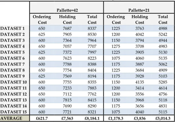
Table 1. Case A costs with L=12, Q=42;21
Pallette=42 Pallette=21 Ordering Cost Holding Cost Total Cost Ordering Cost Holding Cost Total Cost DATASET 1 650 7687 8337 1225 3763 4988 DATASET 2 625 7905 8530 1200 4042 5242 DATASET 3 600 7364 7964 1150 3794 4944 DATASET 4 650 7057 7707 1275 3708 4983 DATASET 5 625 7372 7997 1225 3905 5130 DATASET 6 600 7623 8223 1075 4060 5135 DATASET 7 600 7788 8388 1175 3887 5062 DATASET 8 650 7754 8404 1225 3684 4909 DATASET 9 625 7569 8194 1175 3928 5103 DATASET 10 600 7755 8355 1150 4135 5285 DATASET 11 650 7233 7883 1200 3414 4614 DATASET 12 650 7112 7762 1200 3556 4756 DATASET 13 600 7815 8415 1150 3968 5118 DATASET 14 600 7690 8290 1175 3656 4831 DATASET 15 600 7721 8321 1075 4040 5115 AVERAGE £621.7 £7,563 £8,184.1 £1,178.3 £3,836 £5,014.3
As it is seen in Table 1, the average total cost £8,184 with £621.7 of ordering cost and £7,563 for holding cost with 42 palette quantity. When it is compared to the Q=21 case, it is clearly seen that holding cost is decreasing sharply while there is an increase on ordering cost. The reason of this is that the system keeps more stock on hand and order less when the pallet quantity is large. On overall total cost, there is 39% decrease when the palette quantity is changed to 21 instead of 42. Although, the Q=21 case has better results, performance measures are also required to be considered. Performance measures like service level and average delay are shown in Table 2.
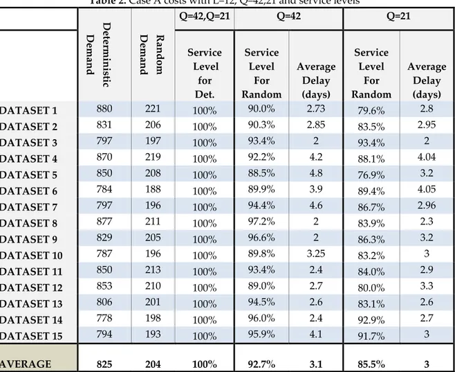
Table 2. Case A costs with L=12, Q=42;21 and service levels Dete rmini st ic Dem and Rando m Dem and Q=42,Q=21 Q=42 Q=21 Service Level for Det. Service Level For Random Average Delay (days) Service Level For Random Average Delay (days) DATASET 1 880 221 100% 90.0% 2.73 79.6% 2.8 DATASET 2 831 206 100% 90.3% 2.85 83.5% 2.95 DATASET 3 797 197 100% 93.4% 2 93.4% 2 DATASET 4 870 219 100% 92.2% 4.2 88.1% 4.04 DATASET 5 850 208 100% 88.5% 4.8 76.9% 3.2 DATASET 6 784 188 100% 89.9% 3.9 89.4% 4.05 DATASET 7 797 196 100% 94.4% 4.6 86.7% 2.96 DATASET 8 877 211 100% 97.2% 2 83.9% 2.3 DATASET 9 829 205 100% 96.6% 2 86.3% 3.2 DATASET 10 787 196 100% 89.8% 3.25 83.2% 3 DATASET 11 850 213 100% 93.4% 2.4 84.0% 2.9 DATASET 12 853 210 100% 89.0% 2.7 80.0% 3.3 DATASET 13 806 201 100% 94.5% 2.6 83.1% 2.6 DATASET 14 778 198 100% 96.0% 2.4 92.9% 2.7 DATASET 15 794 193 100% 95.9% 4.1 91.7% 3 AVERAGE 825 204 100% 92.7% 3.1 85.5% 3
As it is seen in Table 2, the service level for deterministic demand is 100% whereas the average service level for stochastic demand is 92.7%. As the uncertainty on demand increases, the service level decreases as expected. On the other hand, the case of Q=21 has 85.5% service level for random demand. The service level is defined as the units that are backordered over total stochastic demand. Since the shortage cost for deterministic demand is very high, the service level is 100% with Q=42 and Q=21. For each unit backordered for stochastic demand is averagely delivered late about 3.1 days for Q=42 whereas it is 3 days for Q=21. When we compare the cases with 42 and 21 pallet quantities, economically the model with pallet 21 performs better. On the other hand, in terms of the service level, the first case has 92.7% while the other one has 85.5% while average delay time is almost same for both.
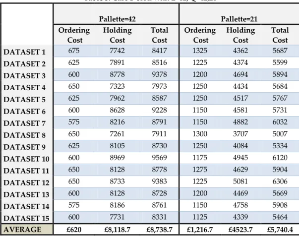
In case B, demands have inverse percentages for the case A. These results are gained with 20% deterministic demand and 80% stochastic demand with running of 15 datasets. The economical results are illustrated in Table 3.
Table 3. Case B costs with L=12, Q=42;21 Pallette=42 Pallette=21 Ordering Cost Holding Cost Total Cost Ordering Cost Holding Cost Total Cost DATASET 1 675 7742 8417 1325 4362 5687 DATASET 2 625 7891 8516 1225 4374 5599 DATASET 3 600 8778 9378 1200 4694 5894 DATASET 4 650 7323 7973 1250 4434 5684 DATASET 5 625 7962 8587 1250 4517 5767 DATASET 6 600 8628 9228 1150 4581 5731 DATASET 7 575 8216 8791 1150 4882 6032 DATASET 8 650 7261 7911 1300 3707 5007 DATASET 9 625 8105 8730 1250 4084 5334 DATASET 10 600 8969 9569 1175 4945 6120 DATASET 11 650 8128 8778 1275 4629 5904 DATASET 12 650 8733 9383 1225 5081 6306 DATASET 13 600 8128 8728 1200 4469 5669 DATASET 14 575 8186 8761 1150 4758 5908 DATASET 15 600 7731 8331 1125 4339 5464 AVERAGE £620 £8,118.7 £8,738.7 £1,216.7 £4523.7 £5,740.4
Similar to results in Case A, lower quantity in pallet brings better results in terms of holding cost. Overall, 34% improvements achieved on total cost by reducing number of computers in a pallet. Comparison of Case A and Case B results for the same parameters, about 8% increase on total costs are faced for both Q=42 and Q=21. Only difference between costs does not give a clear idea unless systems performances are not compared. Table 4 demonstrates performance of Case B with a lead time of 12 days in terms of service level and delay time.
Table 4. Case B costs with L=12, Q=42;21 and service levels Dete rmini st ic Dem and Rando m Dem and Q=42,Q=21 Q=42 Q=21 Service Level for Det. Service Level For Random Average Delay (days) Service Level For Random Average Delay (days) DATASET 1 214 864 100% 85.3% 2.3 77.7% 3.4 DATASET 2 204 808 100% 88.9% 2.5 78.2% 2.7 DATASET 3 196 783 100% 93.4% 2.6 81.1% 4.1 DATASET 4 218 859 100% 81.8% 3.6 71.5% 4.4 DATASET 5 212 843 100% 86.8% 2.3 76.9% 2.7 DATASET 6 192 777 100% 89.2% 3.4 80.1% 2.9 DATASET 7 201 796 100% 86.3% 2.7 80.4% 3.2 DATASET 8 215 875 100% 85.5% 2.5 77.7% 3.1 DATASET 9 202 822 100% 87.5% 3.4 75.5% 2.9 DATASET 10 192 765 100% 83.3% 3.3 77.1% 4.6 DATASET 11 203 841 100% 83.0% 2.94 73.0% 2.6 DATASET 12 212 837 100% 82.1% 3.8 71.8% 3.8 DATASET 13 201 806 100% 92.1% 3.4 83.4% 3.5 DATASET 14 196 762 100% 87.9% 2.13 84.0% 3.6 DATASET 15 191 774 100% 85.8% 3.2 74.9% 3.2 AVERAGE 203 830 100% 86.6% 2.92 77.6% 3.4
In Table 4, it is seen that higher pallet amount gives higher service level for random demand. However, the service measures are worse than the Case A results under same situation.
When we evaluate the results we obtained from the model, we can see that the results are as expected in general. An important result is that the service level is high for random demand when the pallet quantity is large. This indicates that large pallet quantity works like a safety stock. Thus, the inventory policy is changing by the pallet quantity. For large size pallets we expect to have less safety stocks compared to the lower pallet quantities. The effects of other parameters will be detailed in following sections.
4.1. Current Situation Results
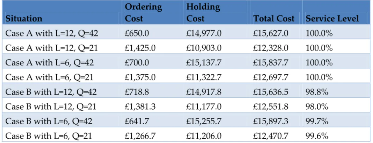
Safety stock is used to manage the inventory system against unexpected demand. In the current situation in the university, reorder level is determined as 20 computers. To see the difference between current system and our model results, the current situation is modelled into VBA. Like the model runs previously, demands are used from Case A and Case B situations. Order amount is always chosen as 1 pallet. If inventory level at the day which is today plus lead time is less than 20, then an order placed on today. Current situation is again run over a year with different data and the average results are presented in Table 5.
Table 5. Current situation average results Situation
Ordering Cost
Holding
Cost Total Cost Service Level
Case A with L=12, Q=42 £650.0 £14,977.0 £15,627.0 100.0% Case A with L=12, Q=21 £1,425.0 £10,903.0 £12,328.0 100.0% Case A with L=6, Q=42 £700.0 £15,137.7 £15,837.7 100.0% Case A with L=6, Q=21 £1,375.0 £11,322.7 £12,697.7 100.0% Case B with L=12, Q=42 £718.8 £14,917.8 £15,636.5 98.8% Case B with L=12, Q=21 £1,381.3 £11,177.0 £12,551.8 98.0% Case B with L=6, Q=42 £641.7 £15,255.7 £15,897.3 99.7% Case B with L=6, Q=21 £1,266.7 £11,206.0 £12,470.7 99.6%
As it is seen, the service level for current situation is nearly perfect. However, the costs are almost double than our model costs. Since the random demand percentage is low in Case A, none of shortages are seen. On the other hand, for the case B very little amount of shortages are observed. Managers need to decide whether it is worthy to keep service level with obtained costs or not. For further research, the optimum reorder level could be investigated which minimizes the cost while keeping the service level on a desirable level.
4.2. Impact of the Parameters
All results are summarized in Table 6 and according to these results; the impacts of parameters are discussed
Table 6. Average results for different situations Situation Ordering Cost Holding Cost Total Cost Service Level Average Delay Deterministic L=12, Q=42 £621.7 £7,208.5 £7,830.2 100% 0 Deterministic L=12, Q=21 £1,106.7 £3,646.9 £4,753.6 100% 0 Case A with L=12, Q=42 £621.7 £7,563 £8,184.1 92.7% 3.1 Case A with L=12, Q=21 £1,178.3 £3,836 £5,014.3 85.5% 3 Case A with L=6, Q=42 £620 £7,590.1 £8,210.1 95.6% 1.9 Case A with L=6, Q=21 £1,181 £3,803.7 £4,985.4 93% 1.7 Case B with L=12, Q=42 £620 £8,118.7 £8,738.7 86.6% 2.92 Case B with L=12, Q=21 £1,216.7 £4523.7 £5,740.4 77.6% 3.4 Case B with L=6, Q=42 £621.7 £7,907.5 £8,529.2 90.2% 1.8 Case B with L=6, Q=21 £1,216.7 £4,184.7 £5,401.4 82.4% 1.85
The decreasing on percentage of deterministic demand results an increase on total cost while the service level is getting lower. It is clearly showed in Table 6 that with L=12 and Q=42 parameters, both of optimum total cost and service level can be obtained for fully deterministic (known in advance) demand. Similar to this result, the runs with L=12 and Q=21 proved advance demand information is the best case. It might be seen that there is no big difference on total costs. However, the changing in service level shows us the importance of advance demand information.
Lead Time
Except fully deterministic case, lower costs and better service level are recorded with lower lead times. Similar to the advance demand information, the main differences can be seen on service levels instead of total costs. It is concluded that lower lead time will bring better service levels for less or equal to costs of the higher lead time.
Pallet Quantity/Batch Ordering
With the higher percentage of deterministic demand, the reduction on pallet quantity causes lower costs with lower service level. In the model, according to the observations, the high amount pallet behaves like safety stock and prevent model to make backorders. Therefore the demand with contains high level of random demand is more likely to give better results with higher amount in pallets.
In summary, choosing parameters are an issue which is related to decision of what level of service level is acceptable with what costs.
5. CONCLUSION
The main purpose of this study is to analyse the past demand and develop an inventory model based on the demand pattern. Due to the lack of data, the past demand analysis could only be made partially. Therefore datasets are generated instead of using real data. For the inventory model, a mathematical formulation is developed which allow the university to manage their stock systems. It is realized that some percentage of demand can be known in advance. Seeing the impact of this advance demand information, different cases are tested with different datasets. Mainly, it concluded that advance demand information is improving the inventory system in terms of both decreasing cost and increasing service level. The reduced lead times has no significant impact on inventory model while all demand is deterministic. While the percentage of random demand is getting higher, the reduced lead time has more impact the deterministic cases. For all cases, pallet obligation increases the cost whereas it increases the service level as well.
Integration of the model with the current stock spreadsheet used by the staff in the university will make the decision process easier. As an application, an appropriate software can be updated with the developed model in this paper for the stock system. In this paper, it is assumed that the lead time is constant. For more realistic case, the varying or stochastic lead times need to be considered and further models can be developed. Also the pallet quantity can be considered as a decision variable and another mathematical model developed to find the optimal pallet size.
REFERENCES
Aloulou, M., Dolgui, A. and Kovalyov, M. (2013). A bibliography of non-deterministic lot-sizing models. International Journal of Production Research, 52(8), pp.2293-2310.
Bon, A. and Leng, C. (2009). The Fundamental on Demand Forecasting in Inventory Management. Australian Journal of Basic and Applied Sciences, 3(4), pp.3937--3943.
Bushuev, M., Guiffrida, A., Jaber, M. and Khan, M. (2015). A review of inventory lot sizing review papers. Management Research Review, 38(3), pp.283-298.
Chao, X. and Zhou, S. (2009). Optimal Policy for a Multiechelon Inventory System with Batch Ordering and Fixed Replenishment Intervals. Operations Research, 57(2), pp.377-390.
Chen, F. (2000). Optimal Policies for Multi-Echelon Inventory Problems with Batch Ordering. Operations Research, 48(3), pp.376-389.
Chen, F. and Zheng, Y. (1994). Evaluating Echelon Stock (R, nQ) Policies in Serial Production/Inventory Systems with Stochastic Demand. Management Science, 40(10), pp.1262-1275.
Gallego, G. and Ozer, Özalp. (2001). Integrating replenishment decisions with advance demand information. Management Science, 47(10), pp.1344--1360.
Kesen, S. E., Kanchanapiboon, A. and Das, S. (2010). Evaluating supply chain flexibility with order quantity constraints and lost sales. International Journal of Production Economics, 126(2), pp.181-188.
Özer, Ö. and Wei, W. (2004). Inventory Control with Limited Capacity and Advance Demand Information. Operations Research, 52(6), pp.988-1000.
Shang, K. and Zhou, S. (2010). Optimal and Heuristic Echelon (r, nQ, T) Policies in Serial Inventory Systems with Fixed Costs. Operations Research, 58(2), pp.414-427.
Sobel, M. and Zhang, R. (2001). Inventory policies for systems with stochastic and deterministic demand. Operations research, 49(1), pp.157--162.
Taha, H. (2007). Operation Research: An Introduction. 8th ed. New Jersey: Pearson, pp.427-449.
Veinott, A. (1965). The Optimal Inventory Policy for Batch Ordering. Operations Research, 13(3), pp.424-432.
Wang, T. and Toktay, B. (2008). Inventory management with advance demand information and flexible delivery. Management Science, 54(4), pp.716--732.
Waters, C. (1992). Inventory control and management. 1st ed. Chichester [England]: Wiley.
Van Woensel, T., Erkip, N., Curseu, A. and Fransoo, J.C., 2013. Lost sales inventory models with batch ordering and handling costs. In Beta Working Paper series. Eindhoven (Vol. 421).