Decomposing linear programs for parallel solution

V

5«ßs

? S ^ I! i

IITI.Ili

4 *■ ύ i ¿ ^ i-i :*.^ \ J >{¿í j ; ,;. ÿ jy ¿ ÿ

DECOMPOSING LINEAR PROGRAMS EOR

PARALLEL SOLUTION

A THESIS

SUBMITTED TO THE DEPARTMENT OF COMPUTER ENGINEERING AND INFORMATION SCIENCE

AND THE INSTITUTE OF ENGINEERING AND SCIENCE OF BILKENT UNIVERSITY

IN PARTIAL FULFILLMENT OF THE REQUIREMENTS FOR THE DEGREE OF

MASTER OF SCIENCE

By

All Pınar

July, 1996

P5é

1936

В Л І 3 5 2 4 5

I certify that I have read this thesis and that in my opin­ ion it is fully adequate, in scope and in quality, as a thesis for the degree of Master of Science.

Assoc. Prof. C e v ^ t Aykanat(Principal Advisor)

I certify that I have read this thesis and that in my opin­ ion it is fully adequate, in scope and in quality, as a thesis for the degree of Master of Science.

I certify that I have read this thesis and that in my opin­ ion it is fully adequate, in scope and in quality, as a thesis for the degree of Master of Science.

st. Prof. Hakan Karaata

Approved for the Institute of Engineering and Science:

ABSTRACT

DECOMPOSING LINEAR PROGRAMS FOR PARALLEL

SOLUTION

All Pınar

M. S. in Computer Engineering and Information Science

Supervisor: Assoc. Prof. Cevdet Ay kanat

July, 1996

Many current research efforts are based on better exploitation of sparsity— common in most large scaled problems— for computational efEciency. This work proposes different methods for permuting sparse matrices to block angular form with specified number of equal sized blocks for efficient parallelism. The problem has applications in linear programming, where there is a lot of work on the so­ lution of problems with existing block angular structure. However, these works depend on the existing block angular structure of the matrix, and hence suf­ fer from unscalability. We propose two hypergraph models for decomposition, and these models reduce the problem to the well-known hypergraph partitioning problem. We also propose a graph model, which reduces the problem to the graph partitioning by node separator problem. We were able to decompose very large problems, the results are quite attractive both in terms solution quality and running times.

Key words: Sparse Matrices, Block Angular Form, Hypergraph Partitioning,

Graph Partitioning by Node Separator

ÖZET

DOĞRUSAL PROGRAM LARIN PARALEL ÇÖZÜMLEME

İÇİN BÖLÜNMESİ

Ali Pınar

Bilgisayar ve Enformatik Mühendisliği, Yüksek Lisans

Danışman: Doç. Dr. Cevdet Aykanat

Temmuz, 1996

Birçok güncel araştırma büyük ölçekli problemlerin matrislerinde sıkça rast­ lanan seyreklikten daha iyi yararlanmaya dayalıdır. Bu araştırma, seyrek bir ma­ trisi belli sayıda eşit büyüklükte bloklardan oluşan blok açısal duruma çevirmek için değişik metodlar önermektedir. Bu problemin önemli bir uygulaması doğrusal programlamadadır. Doğrusal programlamada, varolan blok açısal yapıları kul­ lanan birçok çözüm yöntemi önerilmiştir. Ama bu yöntemler yalnızca varolan blok açısal duruma dayandıkları için ölçeklendirme sorunuyla karşı karşıyadırlar.

Bu çalışma bölünme için iki hiperçizge modeli öneriyor, ve bu modeller prob­ lemi iyi bilinen hiperçizge parçalama problemine indirgiyor. Önerilen bir diğer model ise çizge modeli, ve bu model de problemi düğüm ayıracıyla çizge parçalama problemine indirgiyor. Önerilen modeller, çok sayıda çok büyük ölçekli matris­ leri bölmede denendi. Hem çözüm kalitesi, hem de zaman açısından çok çekici sonuçlar elde edildi.

\nahtar sözcükler: Seyrek Matris, Block Açısal Durum, Hiperçizge Parçalama,

üm Ayıracıyla Çizge Parçalama

Acknowledgment

I would like to express my deep gratitude to my supervisor Dr. Cevdet Aykanat for his guidance, suggestions, encouragement and enjoyable discussions throughout the development of the thesis. I would like to thank Dr. Mustafa Pınar for reading and commenting on the thesis. I would also like to thank Dr. Hakan Karaata for reading and commenting on the thesis. I owe special thanks to all members of the department for providing a pleasant environment for study. Finally, I am very grateful to my family and my friends for their support and patience.

Contents

1 Introduction 1

2 Block Angular Form of a Sparse Matrix 6

2.1 P relim in aries... 6

2.2 Block Angular Systems in Linear P ro g ra m m in g ... 8

3 Graph and Hypergraph Partitioning 11 .3.1 Preliminaries ... 12

3.2 Local Search H e u r is tic s ... 15

3.2.1 Neighborhood Structures for the Hypergraph Partitioning P r o b le m ... 15

3.2.2 H ill-clim bin g... 17

3.2.3 Tie-breaking Strategies ... 17

3.2.4 Hypergraph Partitioning H eu ristics... 18

3.2.5 Alternative S tra teg ies... 25

3.2.6 Multi-start Techniques... 25

3.3 Geometric E m b e d d in g s ... 26

3.4 Multi-level Approaches ... 27

4 Graph Partitioning by Node Separators 30 4.1 Problem D e fin itio n ... 30

4.2 A pplications... 31

4.3 Previous Work for Finding Node Separators... 31

4.3.1 Improving an Initial Separator... 32

4.3.2 Finding a Node Separator from an Edge Separator . . . . 37

4.3.3 New Greedy Heuristics for Finding Separators... 41

CONTENTS

5 Permuting a Sparse Matrix to Block Angular Form 45

5.1 Bipartite Graph Model 46

5.1.1 The Graph M o d e l... 46

5.1.2 B.A.F with Bipartite Graph M o d e l... 47

5.2 Row-Net M o d e l ...

48

5.2.1 The Hypergraph M od el... 49

5.2.2 BAF with Row-Net M o d e l... 50

5.3 Column-Net Model ... 52

5.3.1 The Hypergraph M od el... 52

5.3.2 BAF with Column-Net M o d e l... 52

5.4 Row Interaction Graph 55 5.4.1 The Graph M od el... 56

5.4.2 BAF with Row-Interaction G raph... 56

5.5 Column-Interaction G ra p h ... 57

5.5.1 The Graph M o d e l... 57

5.5.2 BAF with Column-Interaction G rap h ... 58

6 Experimental Results 59 6.1 Data S e t s ... 59

6.2 Implementation of the A lg o r it h m s ... 61

6.3 Experiments with the Bipartite Graph Model 61 6.3.1 Partitioning P h a s e ... 63

6.3.2 Separator P h a s e ... 63

6.4 Experiments with the Row-Net Model ... 66

6.5 Experiments with the Column-Net M o d e l ... 68

6.6 Experiments with the Row Interaction Graph Model ... 70

6.6.1 Validity of Greedy Heuristics 70 6.6.2 Finding Wide Separators... 72

6.7 Comparison of the M odels... 74

7 Conclusion 81 7.1 C o n clu sio n s... 81

7.2 Future W o rk ... 83

CONTENTS

7.2.2 Iterative Improvement Methods for Multi-way Separations 84

7

2..3

A Experimental Results in Detail 92

List of Figures

3.1 A general view of a local search h e u ris tic... 15

3.2 A generalized local search algorithm with h ill-clim b in g ... 18

3.3 Level 1 SN hypergraph partitioning h eu ristic... 23

3.4 Gain computation for a vertex u ... 24

3.5 An overview of Multi-level Hypergraph P artition in g... 29

4.1 Algorithm for Improving an initial s e p a ra to r... 32

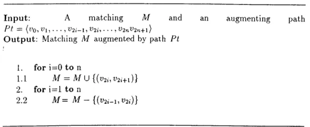
4.2 Algorithm for finding a maximum matching on a bipartite graph . 34 4.3 Algorithm for Augmenting a matching with an augmenting path 35 4.4 Improving matchings via augmenting p a th s... 36

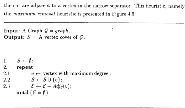
4.5 Algorithm for the Maximum Inclusion Heuristic proposed by Leis-erson and Lewis ... 40

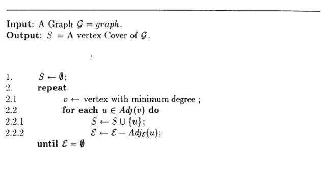
4.6 Algorithm for the Minimum Recover Heuristic proposed by Leis-erson and Lewis ... 41

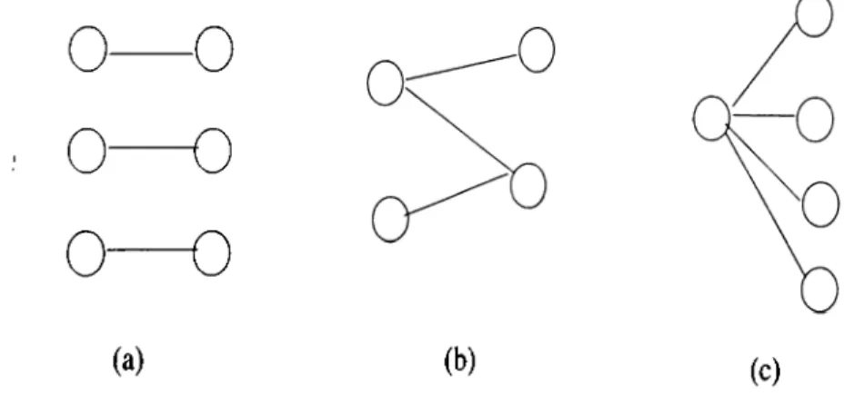
4.7 Three Different Wide separators... 42

4.8 Algorithm for a new greedy heuristic, O n e - M a x ... 44

5.1 The nonzero structure of the matrix A ... 46

5.2 Bipartite Graph Representation of the matrix A in Figure'5.1 . . 47

5.3 Hypergraph Representation of the matrix A in Figure 5.1 with Row-Net M o d e l... 49

5.4 Block angular form of Matrix A in Figure 5.1 50 5.5 Hypergraph Representation of the matrix A in Figure 5.1 with Column-Net M o d e l... 53

5.6 Dual block angular form of matrix A in Figure 5 .1 ... 53 5.7 Matrix A in Figure 5.6 after column-splitting 55

LIST OF FICAIRES

5.8 Block angular matrix A in Figure 5.6 after column splitting and

permutation ... 55

5.9 Row-Interaction Graph Representation of the matrix A in Figure 5.1 56 5.10 Column-Interaction Graph Representation of the matrix A 58 6.1 Comparison of Metis and Sanchis partitioning tools on BG model. Figure display results of 2,4,6, and 8 block decompositions. Mini­ mum and average are results of experiments on 27 different matri­ ces with 20 run for each, the numbers have been normalized with respect to that of PaToH... 64

6.2 Comparison of Greedy Heuristics with BG M o d e l ... 65

6.3 Comparison of PaToH and Sanchis (SN) for RN m o d e l ... 67

6.4 Comparison of PaToH and Sanchis (SN) for CN m o d e l ... 69

6.5 Comparisons of Greedy Heuristics for R I G ... 71

6.6 Comparison of Greedy heuristics with Optimal s o lu t io n s ... 72

6.7 Comparison of Minimum Separator Sizes for different methods 73 6.8 Comparison of Average Separator Sizes for different methods . . . 74

6.9 Comparison of Running Times for different methods 75 6.10 Comparison of best solutions of different m o d e ls ... 76

6.11 Comparison of averages of different m o d e ls ... 77

6.12 Comparison of running times for different m o d e l s ... 78

6.13 Figure gives a general comparison of different models for 2,4,6 and 8 block decomposition of 27 different matrices. The results af­ ter due to average of 20 runs. Values have been normalized with respect to RIG... 79

7.1 Multi-way Separator Improvement Algorithm 85 B .l Matrix GE Original Structure... 119

B.2 Matrix GE after 2 Block Decomposition ...120

B.3 .Matrix GE after 4 Block D ecom p osition ...120

B.4 Matrix GE after 6 Block D ecom p osition ... 121

B.5 Matrix GE after 8 Block D ecom p osition ...121

B.6 Matrix CQ9 Original S tru ctu re... 122

LIST OF FIGURES

Xll

B.8 Matrix CQ9 after 4 Block D e c o m p o s itio n ...123 B.9 Matrix CQ9 after 6 Block D e c o m p o s itio n ...124 B.IO Matrix CQ9 after 8 Block D e c o m p o s itio n ...124

List o f Tables

6.1 Properties of the Problems used in the Experim ents... 60

6.2 Properties of the RIG ’s of Matrices used in the Experiments . . . 62

6.3 The effectiveness of RIG M o d e l ... 80

A .l General Comparison of Sanchis (SN) and M e t i s ... 92

A .2 Comparison of Sanchis (SN) and M e t i s ... 93

A.3 Comparison of Greedy Heuristics with BG M o d e l ... 94

A .4 Comparison of PaToH and Sanchis (SN) for RN m o d e l ... 95

A.5 Comparison of PaToH and Sanchis (SN) for RN model (cont.d) . 96 A .6 Comparison of PaToh and Sanchis (SN) for RN model (cont.d) . . 97

A .7 General Comparison of PaToH and Sanchis on RN M o d e l... 98

A .8 Comparison of PaToH and Sanchis (SN) for CN m o d e l ... 99

A .9 Comparison of PaToH and Sanchis (SN) for CN model (cont.d) . 100 .A. 10 Results of Column-Net with transfer model with P a T o h .101 A. 11 Results of Column-Net with transfer model with PaToh (cont.d) . 102 A. 12 Results of Column-Net with transfer model with PaToh (cont’d) . 103 A. 13 Comparisons of Greedy Heuristics for R I G ...104

A. 14 Comparison of Greedy heuristics with Optimal s o lu t io n s ... 105

A. 15 Comparison of Wide Separators for different m e th o d s ...106

A. 16 Comparison of Edge Cuts for different m e t h o d s ... 107

A. 17 Comparison of Minimum Separator Sizes for different methods . 108 A. 18 Comparison of Average Separator Sizes for different methods . . 109

.A. 19 Comparison of run times for different methods ... 110

A.20 Comparison of separators with weighted and unweighted models . I l l A .21 Comparison of separators with weighted and unweighted models (cont.d) ... 112

LIST OF TABLES

A .22 Comparison of separators with weighted and unweighted models

(cont.d) ...113

A .23 General Comparison of separators with weighted and unweighted models ... : ... 114

A .24 Comparison of different models ... 115

A .25 Comparison of different models (c o n t.d )... 116

A .26 Comparison of different models (c o n t.d )... 117

1. Introduction

Studies on sparse matrices has its origins in diverse fields such as management sci­ ence, power systems analysis, finite element problems, circuit theory, etc. Math­ ematical models in all of these areas give rise to very large systems of linear equations that could not be solved if most of the entries in these matrices were not zeros. This increases the interest in sparsity, because its exploitation can lead to enormous computational savings and because many large problems that occur in practice are sparse.

.An important exploitation of sparsity arises in solving linear systems of equa­ tions. A good ordering of the rows and columns of the matrix can help us to preserve sparsity during factorization. The problem has been heavily studied in the literature because of the significant computational savings and the wide- applicability of the problem. Minimum Degree Ordering [25], Nested dissection [26] are the most popular solution methods of this problem. Other special forms of sparse matrices such as band matrices, block tridiagonal matrices, and block triangular matrices give rise to computational savings and special solution tech­ niques, and permutation into these forms has been studied in the literature [20]. Although ordering sparse matrices to various special forms has been studied in the literature, the problem of permuting rows and columns of a sparse matrix into a block angular form, with specified number of equal sized blocks while min­ imizing the number of coupling rows, remains almost untouched. Solving linear systems of equations with block angular matrices has an inherent parallelism, be­ cause the blocks are independent, and can be handled concurrently. This kind of matrices arise in Linear Programming, such as multi-commodity flow, multi-stage stochastic problems.

('HAPTER 1. INTRODUCTION

Linear Programming (LP) is concerned with the optimization (maximization or minimization) of a linear function, while satisfying a set of linear eciuality and/or inequality constraints, and it is currently one of the most popular tools in modeling economic and physical phenomena where performance measures are to i)e optimized subject to certain requirements. LP was first conceived by George B. Dantzig around 1947. The most popular solution method for linear program­ ming problems is the Simplex Method proposed by Dantzig in 1949. The other popular method is the Interior Point Method proposed by Karmarkar in 1984. Both of these methods have been successfully applied to many LP problems of moderate size. However, the performance of these two methods decreases as the problem size increases. The sizes of the constraint matrices of many LP’s can be extremely large, in practice, which restricts the applicability of the standard so­ lution techniques. This leads to the idea of applying divide-and-conquer schema for solving very large problems. Solving linear programs by decomposition was first proposed by Dantzig and Wolfe [18] in 1960, and has been the subject of many research efforts since then. Problems with block angular constraint ma­ trices are very suitable for applying decomposition techniques. Also solution of these problems with decomposition has an inherent parallelism.

The parallel solution of block angular LP’s has been a very active area of research in both operations research and computer science societies. The most I)opular decomposition technique, Dantzig-Wolfe decomposition has been suc­ cessfully adopted for parallel solution of the block angular LP’s. In this scheme, the block structure of the constraint matrix is exploited for parallel solution in the subproblem phase where each processor solves a smaller LP corresponding to a distinct block. A sequential coordination phase (the master) follows. This cycle is repeated until suitable termination criteria are satisfied. Coarse grain |)arallelism inherent in these approaches has been exploited in many other recent research works [27, 43]. However, the success of these approaches depends only on the existing block angular structure of the given constraint matrix. The num­ ber of processors utilized for parallelization in these studies is clearly limited by the number of inherent blocks of the constraint matrix. Hence, these approaches suffer from unscalabiJity and load imbalance.

CHAPTER 1. INTRODUCTION

This work focuses on the problem of permuting rows and columns of an irreg­ ularly sparse rectangular matrix to obtain block angular structure with specified number of blocks for scalable parallelization. The objective in the decomposition is to minimize the number of coupling rows, while maintaining a balance criterion among the sizes of the blocks. Minimizing the number of coupling rows corre­ sponds to minimizing the sequential component of the overall parallel scheme. Maintaining a balance criterion among the sizes of the blocks corresponds to minimizing processors’ idle time during each subproblem phase.

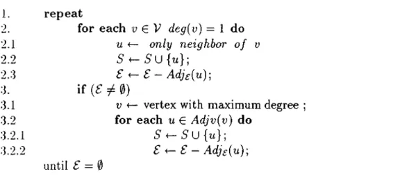
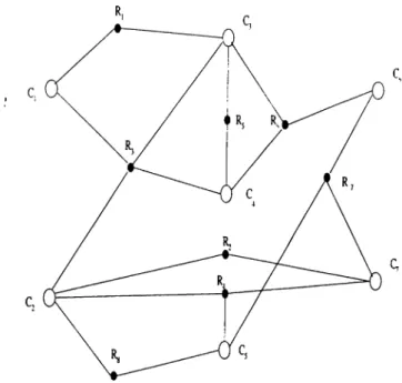
The literature that addresses this problem is extremely rare and very recent. Ferris and Horn [21] model the constraint matrix as a bipartite graph. In this graph, each row and each column is represented by a vertex, and one set of ver­ tices representing rows and the other set of vertices representing columns form a bipartition. There exists an edge between a row vertex and a column vertex if and only if the respective entry in the constraint matrix is nonzero. Ferris and Horn partition this graph using the Kernighan-Lin heuristic [36]. They obtain a node separator from this graph by repeatedly adding the vertex with highest degree to the separator. This enables permutation of the graph into a doubly bordered block angular form. Out of the vertices in the separator, ones repre­ senting the columns constitute the row-coupling columns, and ones representing the rows constitute the column-coupling rows. This doubly bordered matrix can be transformed into a block angular matrix by column splitting, a technique sim­ ilar to the one used in stochastic programming to treat non-anticipativity [44]. This model naturally leads to a doubly bordered block angular matrix, and does not reduce the problem to any well-studied combinatorial optimization problem.

In this work, we propose three different models for representing sparse ma­ trices for decomposition. Each model reduces the problem to a well-studied combinatorial optimization problem. In the first two models, we exploit hyper­ graphs to model matrices for decomposition. A hypergraph is defined as a set of vertices (nodes) and a set of nets (hyperedges) between those vertices. Each net is a subset of the vertices of the hypergraph. A graph is a special instance of a hypergraph, where each net contains exactly two vertices.

In the first model— referred to here as the row-net model— each row is rep­ resented by a net, whereas each column is represented by a vertex. The set

CHAPTER 1. INTRODUCTION

of vertices connected to a net corresponds to the set of columns which have a nonzero entry in the row represented by this net [48]. In this case, the decomposi­ tion problem reduces to the well-known bvpergraph partitioning problem which is known to be NP-Hard [24]. Hypergraph partitioning tries to minimize the number of nets on the cut, while maintaining balance between the parts. Main­ taining balance corresponds to balance between sizes of the blocks in the block angular matrix, and minimizing the number of nets on the cut corresponds to minimizing the number of coupling rows in the block angular matrix.

The second model— referred to here as the column-net model— is very similar to the row-net model, only the roles of columns and rows are exchanged. Each column is represented by a net, whereas each row is represented by a vertex. The set of vertices connected to a net corresponds to the set of rows which have a nonzero entry in the column represented by this net [48]. Applying partitioning on this hypergraph can be considered as permuting the rows and columns of this matrix to dual block angular form. This dual block angular matrix achieved by hypergraph partitioning can be transformed into a block angular form by using column-splitting [44].

Hypergraph partitioning has been heavily studied in VLSI design automation, and many heuristics have been proposed for this problem. In this study, we make use of different heuristics originally proposed for VLSI partitioning, and adapt these heuristics for decomposing matrices.

In our third model— referred to here as the Row Interaction Graph model— each row is represented by a node, and there is an edge between two nodes if there exists a column which has nonzeros in both respective rows [47]. This model reduces the decomposition problem into the graph partitioning by node separator problem. Nodes in part P{ of a partition correspond to the rows in block Bi, and nodes in the separator correspond to the coupling rows. Hence, minimizing the number of nodes in the separator corresponds to minimizing the size of the master problem. By definition of the node separator, there are no edges between nodes in different parts, hence there is no interaction among rows of different blocks.

CHAPTER /. INTRODUCTION

matrices to preserve sparsity during factorization. Besides utilizing present meth­ ods for decomposition, this work includes contributions for finding better node separators on graphs.

VVe have demonstrate the validity of the proposed graph model with various linear program constraint matrices selected from NETLIB and other sources. We were able to decompose a matrix with 10099 rows, 11098 columns, 39554 nonzeros into 8 blocks with only 517 coupling rows in 1.9 seconds and a matrix with 34774 rows, 31728 columns, 165129 nonzeros into 8 blocks with only 1029 coupling rows in 10.1 seconds. The solution times with LOQO are 907.6 seconds for the former and 5970.3 seconds for the latter. These results are quite promising and our decomposition techniques form feasible decompositions for parallel solution.

The organization of this thesis is as follows: Chapter 2 includes a definition of block angular matrices and their applications. Chapter 3 presents a brief description of hypergraphs and the hypergraph partitioning problem. We use the terminology described in this section throughout the thesis. This chapter also reviews different approaches proposed for hypergraph partitioning problem such as local search methods, geometric embeddings, multi-level approaches and multi­ start techniques. Chapter 4 defines the graph partitioning by node separators problem, and reviews the previous work. New methods that can help us to find better separators are also presented in this chapter. Chapter 5 describes the tour models for permuting matrices to block angular form. We review the bipartite graph model of Ferris and Horn, and propose row-net, column-net, and row interaction graph models. Chapter 6 presents our experimental results, and comparisons of different models and methods, and comments on the experimental results. Finally, we give directions for future work and conclude the thesis in Chapter 7.

2. Block Angular Form of a Sparse Matrix

Block angular systems have been attractive for computer scientist due to their inherent parallelism. The blocks of the system can be handled concurrently, since they are independent. Below, we will define block angular systems, and we will discuss some of the applications.

2.1

Preliminaries

In this section, we will define block angular matrices. Definitions 2.1-2.4 have been taken from [21].

D e fin itio n 2.1 A matrix A € is said to be in block angular form if it has the following structure:

A =

Bx

\

B o

Bk

^ R\ · · · Rk j

where Bi G . Each submatrix Bi is called a block, and

k k

M + q and A" = ^ n , .

1=1 1=1

D e fin itio n 2.2 A matrix A € is said to be in dual block angular form if it has the following structure:

4 “ — /ig — Bx B o

Cx

Bk Ck

\

CHAPTER 2. BLOCK ANGULAR FORM OF A SPARSE MATRIX

where G , , C,· G Each submatrix Bi is called a block, and

M = ^2 _{o,nd N = '^ r ii -\- P}

1=1 1=1

I

D e fin itio n 2.3 A matrix A G is said to be in doubly bordered block

angular form if it has the following structure:

^DB = B , C l C2 \ Bk Ck Rl i?2 Rk D y

where Bi G C,· G Ri G and D G Each submatrix

Bi is called a block, and

k k

M = ^ 2 m i + q and ^ + p .

1=1 1=1

D e fin itio n 2.4 Each row o f the q x N submatrix

{Rl i?2 · · · Rk D)

is called a column-linking or column-coupling row.

Generally, column-linking rows restrict the column spaces of the blocks, re­ sulting in the column space for the entire matrix. A column-linking row may restrict the column space of one block Bi based on the column space of another block B j . In this case, the blocks Bj and Bj are said to be linked or coupled by this row.

D e fin itio n 2.5 Each column o f the M x p submatrix

I Cl ^

C2

Ck \ ^ } is called a row-linking or row-coupling column.

Generally, row-linking columns restrict the row spaces of the blocks, resulting in the row space for the entire matrix. A row-linking column may restrict the row space of one block Bi based on the row space of another block B j. In this case, the blocks Bi and Bj a,r'e said to be ¡inked or coupled by this column.

CHAPTER 2. BLOCK ANGULAR FORM OF A SPARSE MATRIX

8

2.2

Block Angular Systems in Linear Programming

Linear Programming (LP) is concerned with the optimization (maximization or minimization) of a linear function, while satisfying a set of linear equality and/or inequality constraints. The linear programming problem was first conceived by George B. Dantzig around 1947.

A linear program has the canonical form

M in im ize Subject to cix i + _C2X2 + . . . + CnXfi O i i X i + 0 12X2 + . . . + ^In^n > bx 0 21X1 + 022^2 + . . . + _{(^2n^n > f>2} O m l ^ J l + dm2X2 + · · · + dmn^n > bm X l _X2 7 Xn > 0

Here ciX\ + C2X2 + . . . + c„x „ is the objective function, Ci,C

2

objective coefficients, and Xi,X2, . . . , X n are decision variables to be determined.

The inequality Yjj=iUijXj > bj denotes the fth constraint. The coefficients a,j for i = 1,2, . . . , m , and j = 1,2, . . . , n are called the technological coefficients, and they form the constraint matrix A.

/

\

The column vector whose eth component is 6, , which is referred to as the right-

hand side vector represents the minimal requirements to be satisfied. Hence,

CHAPTER 2. BLOCK ANGULAR FORM OF A SPARSE MATRIX

M inim ize cTx Subject to A^x > b

X > 0

Every LP problem has an associated dual pi'oblem. The dual problem for the foregoing problem can be stated as :

M axim ize b^y Subject to AJy < c

y > 0

A set of variables x\^X2i . . . iXn satisfying all the constraints is called a feasible point. The set of all such points constitutes the feasible region. Using these

definitions, the linear programming problem can be stated as follows: Among all

feasible points, find one that minimizes (or maximizes) the objective function [4].

The most popular solution method for linear programming problems is the “Simplex Algorithm” , which was proposed by Dantzig in 1949. It has been widely accepted for its simplicity to understand and implement, and its speed in small sized problems. It is a local search algorithm, and moves from one extreme point to another, and it finds the optimal solution, since the set of feasible points is a convex set. The asymptotic complexity of the algorithm is exponential in the worst-case.

Another popular method for solving linear programming problems is the in­

terior point methods, which started with the pioneering work of Karmarkar in

1984 [34]. As the name implies this method moves in the inner space of the fea­ sible region, and finds an optimal solution. The important point in Karmarkar’s method is its polynomial asymptotic complexity.

The performance of both methods decreases as the problem size increaises. Also memory becomes restrictive for large problems. This leads to the idea of solving linear programs by decomposition. The first decomposition scheme was proposed by Dantzig and Wolfe in 1960 [18]. In this scheme, the problem is decomposed into subproblems. Each time a subproblem is solved, and the results are used in the solution of the forecoming subproblems.

CHAPTER 2. BLOCK ANGULAR FORM OF A SPARSE MATRIX

10

these subproblems can be solved concurrently, since they are independent. Multi­ commodity flow, multi-item production scheduling, economic development prob­ lems and multi-stage stochastic problems has block angular constraint matrices

Starting with the pioneering work of Dantzig and Wolfe in 1960 [18], solution of block angular problems (either in parallel or in serial) has been an active area of study, and lead to several studies. Bender decomposition [5], Bundle- based decomposition [43], Alternating Directions Method [38] are examples of such work.

However, the literature addressing how to obtain a block angular structure of a sparse matrix is very rare and recent. Solution methods for this problem will be discussed in Chapter 5.

3. Graph and Hypergraph Partitioning

The importance and popularity of the graph partitioning problem is mostly due to its connection to the problems whose solution depend on the divide-and-conquer paradigm. A partitioning algorithm partitions a problem into semi-independent subproblems, and tries to reduce the interaction between these subproblems. This division of a problem into simpler subproblems results in a substantial reduction in the search space. Graph Partitioning is the basis of hypergraph partitioning, which is more general and more difficult. Graph partitioning has a number of important applications. An exhaustive list of these applications combined with the relevant references is given below.

• VLSI placement [41] • VLSI routing [57]

• VLSI circuit simulation [1]

• memory segmentation to minimize paging [.36]

• mapping of tasks to processors to minimize communication [10] • efficient sparse Gaussian elimination [26]

• laying out of machines in advanced manufacturing systems [56] Some applications of the hypergraph partitioning problem are listed below:

• VLSI placement [22] • VLSI routing [53]

CHAPTER 3. GRAPH AND HYPERGRAPH PARTITIONING

VVe can extend the adjacency definition of a vertex to adjacency definition of a set of vertices K C V as follows:

Adj(V) = U Adj{v) - V . vev

We use Adj{ v, U) to denote the set of vertices adjacent to v in t/.

Adj{v, U) = A d j { v ) n U .

Extending this definition to sets, we can say

Adj{V,U) = A d j { V ) n U .

We will use Adjsiv) to denote the set of edges adjacent to vertex v.

Adjs{v) = {e|e € € and (e = (u,u) or e = ( u, u ) ) } .

For hypergraphs 7i = ( V, W) (also for graphs), a weight function can be defined to map each vertex to a positive number. A similar function can be defined to map nets to positive numbers. We will call the former function the weight function, the latter function as the cost function. We can extend the definition of cost and weight functions for sets as follows:

weight{V') = ^ weight{v) f o r all C V

u€V'

cost{J\f) = ^ cost{n) f o r all f f ' C A f n€V'

Below we will discuss the definition of partitioning for hypergraphs.

D efin ition 3.1 P = {Pi, P2, ■ ■ · ■, Pk} is a k-way partition o f hypergraph H =

(V,A^) if and only if the following three conditions hold:

• Pi C V and Pi ^ fo r i < i < k

• UL, c. = V

CHAPTER 3. GRAPH AND HYPERGRAPH PARTITIONING

14

When k = 2 this partition is called as a bisection or a bipartition.

For a partition F , a net n is said to be internal in partition F , if and only if Vy G n, V Ç. Pi or n f] Pi = n

The set of internal nets A*/ is defined as

Ai[ = {n|ri. is an internal net in a part}

or

Ail = {n|n n F = n f o r n e Ai and Pi G F }

and the set of external nets A/e is defined as

Afs — {n\n n F

7

There are different functions for the cost of a cut. Two of these are widely used. I'he first one is the number of nets on the cut. In this metric cutsize C{P) can be defined as:

C{P) = ^ cost{n) = cost{AfE) = cost{Af) — cost{Aii)

The second metric is the connectivity metric. The connectivity of a net is equal to the number of parts it connects. Formally, connectivity of net con(n) is

con{n) = |{F :

1

7

~ con(n)

n€AT

A partition is balanced if all parts have about the same weight. When all parts have exactly the same weight, we call this partitioning as perfectly balanced. A formal definition for the balance criterion can be expressed as :

W max - Waavg

w

< e

where Wmax is the weight of the part with maximum weight, Wavg is the average weight of parts (i.e., W a v g and e is a predetermined imbalance ratio.

In the light of the definitions above we can define the hypergraph partitioning problem as finding a balanced partition F which minimizes the cost function

CHAPTER 3. GRAPH AND HYPERGRAPH PARTITIONING

15

3.2

Local Search Heuristics

Local search heuristics are very popular for solving combinatorial optimization problems, since they can be easily implemented apd they can be very fast. A general overview of a local search heuristic is given in Figure 3.1. A local search heuristic starts with a random feasible solution, then iteratively improves this solution by moving to solutions in the neighborhood space. This leads to two critical points for local search methods: definition of a neighborhood space and how to choose the neighbor to move within this space. This section discusses neighborhood structures and various methods proposed for the solution of the graph and hypergraph partitioning problems.

In p u t : A combinatorial optimization problem O u tp u t : A local optimum solution

1. generate an initial feasible solution s for the problem 2. re p e a t

2.1 Find a neighbor s' of s with cost(s) > cost(s') 2.2 s s'

until no improvement on s is possible.

Figure 3.1. A general view of a local search heuristic

3.2.1

Neighborhood Structures for the Hypergraph Par­

titioning Problem

The most critical part of a local search heuristic is the neighborhood definition. .After the definition of the neighborhood structure second critical choice is how to choose a neighbor s' for a solution s from the neighborhood N{ s) . Generally there are three ways:

• First descent method chooses the first neighbor in N (s) that has a better cost than s.

CHAPTER 3. GRAPH AND HYPERGRAPH PARTITIONING

16

• Steepest descent method chooses the neighbor st which gives the best cost among all solutions in N( s) .

• Random descent method chooses a neighbor randomly among solutions in

N{3).

First descent method is faster than the steepest descent method, however steepest descent has a higher chance to produce better results.

There are two popular neighborhood structures for the graph partitioning problem. The first is the Swap-Neighborhood and the second is the Move-

Neighborhood. Below, we will discuss these two neighborhood structures. • Swap-Neighborhood:

In this neighborhood structure, two partitions are neighbors if one partition can be obtained from another by swapping two vertices between different parts in one of the partitions. Formally,

Definition 3.2 Let H = (V,A^) be a n-vertex hypergraph and P , P' two k-way partitions o f H . Then, the partition P = ( P i , . . . , P , , . . . , P , , . . . , P^) and the partition P' = ( P i , . . . , (P, —{ u } ) U { u } , . . . , (Pj —{ u } ) U { y } , . . . , Pt) are neighbors fo r some vertices v ^ Pi, u E P j.

The partition P has {k{k — l ) / 2 ) ( n / t ) ^ neighbors if each part has n/k vertices.

• M ove-Neighborhood:

A partition P = ( P i , . . . , Pfc,. . . , P / , . . . , Pk) has a move-neighbor partition P ' if P' can be obtained from P by moving a vertex from one part to another in P . Formally,

Definition 3.3 Let Ti = {V,Af) be a n-vertex graph and P , P' two k- way partitions of 7i. Then, the partition P' = ( P i , . . . , P, — { u } , . . . , Pj U { u } , . . . , Pit) is a move-neighbor o f the partition P = ( P i , . . . , P , , . . . , P j , . . . , Pj·)

fo r some P,, Pj G P and for some vertex v € Pi ■

The partition P has at most k{k — l){n/k) = n{k — 1) neighbors if each part has n/k vertices.

CHAPTER 3. GRAPH AND HYPERGRAPH PARTITIONING

17

The Swap-Neighborhood space of a partition is larger than its Move-Neighborhood, which enables a better search in neighborhood of a solution. However, search­ ing the swap-neighborhood takes more time compared to searching the move- neighborhood. Different algorithms using these two neighborhood spaces will be described in Section 3.2.4.

3.2.2

Hill-climbing

Local search heuristics can be supported with a hill-climbing feature. Suppose the problem is a minimization problem, and cost{s) denotes the cost of the solution s. If we choose sf with cost{s/) < cost{s), this will be a downhill step. On the other hand, if we choose s/ with cost(sf) > cost{s), this will be an uphill step. .Mlowing uphill moves enables the heuristic to escape from being trapped in a local optima. In hypergraph partitioning, generally all possible moves (swaps) are examined and only a prefix of the moves (a consecutive subset of the moves starting with the first move) giving the best solution are realized. This enables us to escape from local óptimas and find better partitions. A local search heuristic with hill-climbing is given in Figure 3.2.

3.2.3

Tie-breaking Strategies

A critical decision in the iterative improvement methods is the choice of the vertex to move (vertex pair to swap). Most of the time, there is more than one vertex, which gives the same improvement. Hagen et. al. [28], observe that 15 to 30 vertices typically share the highest gain value at any time during an FM pass on a VLSI circuit with 833 modules (Primaryl). This shows that an intelligent tie-breaking mechanism can make significant improvements on the overall performance of the partitioning algorithm.

One simple decision is to use LIFO, FIFO or random strategy to choose the vertex to move, out of the highest gain moves. Hagen et. ah, experimented with these three strategies and showed that LIFO strategy significantly overperforms the other two [28]. One explanation for this success will be that LIFO enforces '‘locality” for choosing vertices to move. That is, vertices that form a natural cluster will probably move sequentially.

CHAPTER 3. GRAPH AND HYPERGRAPH PARTITIONING

18

In p u t: A combinatorial optimization problem O u tp u t: A local optimum solution

1 generate an initial feasible solution s for the problem 2 rep ea t

2.1 for a limited number of iterations d o

2.1.1 select the best neighbor sf of in N {s). 2.1.2 s ^ s'

2.3 find the prefix of steps from the loop above, which leads to the best solution in this pass.

2.4 if the prefix is non-empty, th en 2.4.1 realize the steps in this prefix. 2.5 else a local optimum has been found,

until a local optimum has been found.

Figure 3.2. A generalized local search algorithm with hill-climbing

Another method for tie-breaking is to consider not only the gain for that move, but also some possible gains for the future moves. Krishnamurthy introduced a

gain vector, which is a sequence of potential gain values corresponding to gains

of possible moves in the future. The rth entry in the gain vector considers the gain r moves ahead. Ties are broken by first considering first level gain, then the second level gain, etc.

Hagen et. al.[28], introduces a similar look-ahead ability by improving Krish- namurthy’s gain computation with the basic idea behind the success of LIFO structure.

All these studies show the importance of tie-breaking strategies for iterative improvement methods. This is still a hot topic for hypergraph partitioning prob­ lem.

3.2.4

Hypergraph Partitioning Heuristics

In this section, we will overview different hypergraph partitioning heuristics, which use a local search strategy.

CHAPTER 3. GRAPH AND HYPERGRAPH PARTITIONING

19

3.2.4.1 Kernighan-Lin’s Approach

Kernighan-Lin (KL) heuristic was originally proposed for the graph partitioning problem. This heuristic is a local search algorithm and has become the basis of many graph and hypergraph partitioning heuristics [36]. KL heuristic uses a Swap-Neighborhood structure (described in Section 3.2.1). In this neighborhood structure, two partitions are neighbors if one partition can be obtained from another by swapping two vertices between different parts in one of the partitions.

This heuristic assumes that every vertex heis the same weight. It works as follows: first, an initial partition is generated. We then determine the vertex pair whose swap results in the largest swap gain, i.e., the largest decrease in the cutsize or the smallest increase (if no decrease is possible). This pair is tentatively interchanged and locked. The locking prohibits them from taking part in future swaps in this pass. Then, we look for a second pair of vertices whose interchange improves the cutsize the most, and do the same for this pair also. We continue in this way, but we keep a record of all tentative swaps and their gains. We finish when all the vertices are locked. At this time, we have interchanged both parts and are back to the original (initial) cutsize. Starting with the first swap in the record, we perform the subsequence of swaps which result in the smallest cutsize. The following pass begins with unlocking all vertices and proceeds in the same maimer. These passes are repeated until there is no improvement in the cutsize which corresponds to a locally minimum partition.

KL heuristic allows uphill moves to reduce the danger of being trapped in a poor local minimum. This feature of the heuristic enables it to produce bet­ ter partitions than the heuristics that employ only downhill moves. Also, this algorithm is quite robust. We can accommodate additional constraints such as partitioning into unequal-sized parts, required parts for certain vertices. However, it has some disadvantages. The algorithm handles only identical vertex weights. This restricts the applicability of this heuristic. The algorithm has a complexity of O(ii'^lgn) per pass for a graph with n vertices. It has been observed that the algorithm performs poorly on sparse graphs. Furthermore, the quality of the solution generated by this heuristic strongly depends on the initial partition, just like any other local .search partitioning method.

CHAPTER 3. GRAPH AND HYPERGRAPH PARTITIONING

20

In'pergraph partitioning with this heuristic was done by transforming the hyper­ graph to a graph. Later, Schweikert and Kernighan improved this method to handle hypergraphs [55]. A recent study by Dutt decreased the worst-case com ­ plexity of the KL algorithm to 6(^max[\£\d, \£\ Ig |V|)) and average complexity to

0{\E\ Ig |V|), where d is the maximum vertex degree in Q .

3.2.4.2 Fiduccia-Mattheyses’ Approach

Fiduccia-Mattheyses (FM) heuristic [22] was originally proposed for the hyper­ graph partitioning problem, but it can be applied to the graph partitioning prob­ lem as well. This algorithm introduces the Move-Neighborhood structure instead of the swap-neighborhood structure.

In addition, an efficient data structure called the bucket list data structure is proposed. This data structure helps to sort the vertices with respect to their move gains, in time linear in the number of the vertices and keep the vertices in a sorted order according to their move gains, during the partitioning iterations. Moreover, it reduces the time complexity of the KL heuristic to 0 (]F ] + |£^|)· These features of FM heuristic, made it the basis for many of the heuristics that followed.

3.2.4.3 Krishnamurthy’s Approach

This heuristic [39] is an extension of FM ’s method. Look-ahead ability is added to the cell gain concept by considering the number of pins of a net in a part. Each node has a gain vector with size /, where I is the number of levels. First level gain is the same as that in FM’s method. Second level gain shows the possible cutsize reduction in the next move which follows the current cell move. If a net has 2 cells in part P i, and at least one cell in other part P-2, moving one of the two cells from Pi to

/2

CHAPTER 3. GRAPH AND HYPERGRAPH PARTITIONING

3.2 .4.4 Sanchis’ Approach

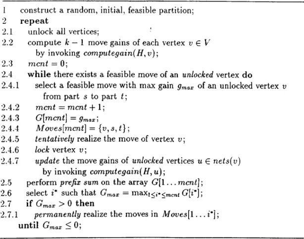
Sarichis [54] generalized Krishnamurthy’s algorithm to a multi-way hypergraph partitioning algorithm so that it could directly handle the partitioning of a hy­ pergraph into more than two parts. All the previous approaches before Sanchis’ algorithm (SN algorithm) are originally bipartitioning algorithms. Level 1 SN algorithm is briefly described here for the sake of simplicity of presentation. De­ tails of SN algorithm which adopts multi-level gain concept can be found in [54]. In SN algorithm, each vertex of the hypergraph is associated with { k - l ) possible moves. Each move is associated with a gain. The move ga,in of a vertex u, in part s with respect to part t i.e., the gain of the move of u,· from the home (source) part s to the destination part i, denotes the amount of decrease in the number of cut nets (cutsize) to be obtained by making that move. Positive gain refers to a decrease, whereas negative gain refers to an increase in the cut- size. Figure 3.3 illustrates the pseudo-code of the SN based ¿-way hypergraph partitioning heuristic. In this figure, nets{v) denotes the set of nets incident to vertex v. The algorithm starts from a randomly chosen feasible partition (Step 1), and iterates a number of passes over the vertices of the hypergraph until a locally optimum partition is found (repeat-loop at Step 2). At the be­ ginning of each pass, all vertices are unlocked (Step 2.1), and initial ¿ — 1 move gains for each vertex are computed (Step 2.2). At each iteration (while-loop at Step 2.4) in a pass, a feasible move with the maximum gain is selected, tentatively performed, and the vertex associated with the move is locked (Steps 2.4.1-2.4.6). The locking mechanism enforces each vertex to be moved at most once per pass. That is, a locked vertex is not selected any more for a move until the end of the pass. After the move, the move gains affected by the selected move should be updated so that they indicate the effect of the move correctly. Move gains of only those unlocked vertices which share nets with the vertex moved should be updated. Gain re-computation scheme is given here instead of gain update mechanism for the sake of simplicity in the presentation (Step 2.4.7). At the end of each pass, we have a sequence of tentative vertex moves and their respective gains. We then construct from this sequence the maximum prefix subsequence of moves with the maximum prefix sum (Steps 2.5 and 2.6). That is, the gains of the moves in the maximum prefix subsequence give the maximum decrease in the

CHAPTER 3. GRAPH AND HYPERGRAPH PARTITIONING

outsize among all prefix subsequences of the moves tentatively performed. Then, vve permanently realize the moves in the maximum prefix subsequence and start the next pass if the maximum prefix sum is positive. The partitioning process terminates if the maximum prefix sum is not positive, i.e., no further decrease in the outsize is possible, and we then have found a locally optimum partitioning. Note that moves with negative gains, i.e., moves which increase the outsize, might be selected during the iterations in a pass. These moves are tentatively realized in the hope that they will lead to moves with positive gains in the following it­ erations. This feature together with the maximum prefix subsequence selection brings the hill-climbing capability to the KL-based algorithms.

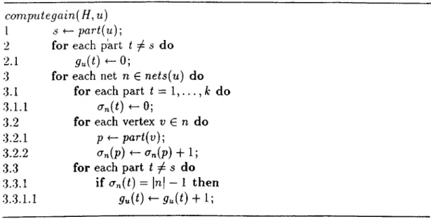
Figure 3.4 illustrates the pseudo-code of the move gain computation algorithm for a vertex и in the hypergraph. In this algorithm, part{y) for a vertex u € V denotes the part which the vertex belongs to, and <t„ (î) counts the number of pins of net n in part t . Move of vertex и from part s to part t will decrease the cutsize if and only if one or more nets become internal net(s) of part t by moving vertex и to part t. Therefore, all other pins (|n| — 1 pins) of net n should be in part t. This check is done in Step 3.3.1.

In this heuristic, each part contains k — l bucket lists; one for each other part, a vertex can move. The time complexity of one pass is 0 {l.p .k{lgk -(- Gmax-l)), where / is the number of levels and Gmax is the size of buckets.

3.2.4.5 Simulated Annealing

Simulated Annealing (SA) was proposed by Kirkpatrick [37] as an optimization method, which heis the capability to escape from local minima. To solve a com­ binatorial optimization problem with SA, a neighborhood structure should be defined for the solution space. Then SA starts with an initial solution, picks a random neighbor of the current solution and moves to this neighbor if it repre­ sents a downhill move. Even if the new solution represents an uphill move, SA will move to it with probability , and stay in the current solution otherwise. Here 6 is the improvement in the cost function of the problem, and T is the current value of the Temperature parameter. To control the rate of convergence and the way of searching the solution space, typically temperature schedule is

CHAPTER 3. GRAPH AND HYPERGRAPH PARTITIONING

23

1 construct a random, initial, feasible partition;

2 repeat

2.1 unlock all vertices;

2.2 compute A: — 1 move gains of each vertex v by invoking com putegain(H ,v);

2.3 merit = 0;

2.4 while there exists a feasible move of an unlocked vertex d o

2.4.1 select a feasible move with max gain Qmax of an unlocked vertex v from part s to part t ;

2.4.2 ment — merit + 1;

2.4.3 G[mcnt] = gmax]

2.4.4 M oves[mcnt] = {v,s,t}'·,

2.4.5 tentatively realize the move of vertex u;

2.4.6 /ocA: vertex u ;

2.4.7 update the move gains of unlocked vertices и € net${v)

by invoking com putegain{H ,u);

2.5 perform prefix sum on the array (?[1.. . m ent]; 2.6 select i* such that Gmax = niaxi<,-.<mcni (?[**];

2.7 if Gmax > 0 then

2.7.1 permanently realize the moves in M o v e s [l. . . ¿*]; until Gmax — H j

Figure 3.3. Level 1 SN hypergraph partitioning heuristic

established, which modifies T as a function of current status of the search pro­ cess (e.g., the number of moves). It has been shown that SA will converge to a globally optimum solution given an infinite number of moves and a temperature schedule that cools to zero sufficiently slowly. The terms “cooling” and “tem­ perature schedule” are due to SA’s analogy to physical annealing of a material into a ground-state energy configuration. One problem with SA is, at low tem­ peratures, many candidate moves might be generated and rejected before one is finally accepted, significantly increasing the run-time.

SA overperforms, in the quality of cutsize, all the previous explained KL-based approaches. However, its run-time is too large, which makes it impractical.

CHAPTER 3. GRAPH AND HYPERGRAPH PARTITIONING

24

computegain{ H, u)

1 if <— part{u);

2 for each part t ^ s do

2.1 g u {t)^ 0 ·,

3 for each net n G nets{u) d o 3.1 for each part i = 1 , . . . , ^ d o

3.1.1

<Tn(0^0;

3.2 for each vertex n G n d o

3

2.1

3.2.2 cr„(p) <- cr„(p) + 1; 3.3 fo r each part < ^ 5 d o 3.3.1 if o-n(t) = |n| — 1 then

3.3.1.1

Figure 3.4. Gain computation for a vertex u

3.2 .4.6 Mean Field Annealing

Mean Field Annealing (MFA) is a technique similar to SA which also has a physical analogy to systems of particles in thermal equilibrium. It was first applied to graph partitioning by Van den Bout and Miller [19]. They use an indicator vector of size |V| to denote a bipartitioning solution, where xi = 0 corresponds to placing u, in the first part, and = 1 corresponds to placing v, in the second part. However, the value of x, varies between 0 and 1. Initially, each X, is set to a value slightly greater than 0.5. Next, a random vertex u, is selected iteratively, and two solutions x(0) which places x,· in the first part, and x ( l) which places x, in the second part are considered. Then the value of x, is updated as:

a;. = (1 + g (F (f(D )-F (i(0 )))/r)-i

The intuition behind this calculation is x, approaches its natural value after each update (i.e., x,· approaches to 1 iff F (x (l)) < < F (x (0 )), and to 0 iff F(.r(0)) « F (x ( l) ) ) .

The process of computing a new x, for randomly chosen v, is repeated until a stable solution is reached. The temperature T is then lowered and the process

CHAPTER 3. GRAPH AND HYPERGRAPH PARTITIONING

₂₅

is repeated, moving x, values further to 0 or 1. Finally, a graph bipartitioning solution can be obtained by rounding each x, to its nearest discrete value. Bultan and Aykanat have extended this basic approach to multi-way partitioning of hypergraphs [9, 10].

The quality of MFA solutions are competitive with those of SA, but usually takes less time than SA, but MFA is still slower than KL-based approaches.

3.2.5

Alternative Strategies

A possible weakness of the KL and FM strategies lies in the locking mechanism, e.g., a module v may be moved from Pi to Pj early in a pass, but its neighbors in P

2

3.2.6

Multi-start Techniques

As discussed in previous sections, iterative improvement heuristics are usually very fast, however they have a high tendency to be trapped in local minima. On the other hand. Simulated Annealing (SA) is very slow, but it is guaranteed to find a global optimum (given infinite time), and in practice SA overperforms other heuristics in quality of the solution at the expense of large amounts of CPU time.

One alternative to SA is a multi-start technique, running iterative improve­ ment heuristics several times, each time starting from a different initial solution, and return the best result. This technique makes a significant improvement on the performance of iterative methods. Also, multi-start technique has a trivial parallelism, which gives an important advantage if the problem is a preprocessing step for a parallel application.

CHA PTER 3. ORAPH AND HYPERGRAPH PARTITIONING

26

the problem size increases. Boese et. al. [6], proposed an adaptive multi-start technique. The technique depends on using the knowledge obtained from previous solutions. One way is to group vertices, that have been placed in the same part, on previous runs for the initial partition. An alternative way is to form clusters of vertices that have been placed in the same part in all previous runs. Studies with adaptive multi-start techniques report improvements compared to pure multi­ start techniques, especially for the average Ccise performance.

3.3

Geometric Embeddings

A geometric representation of the hypergraph can provide a useful basis for a partitioning heuristic, since speedups and special “geometric” heuristics become possible. For example computing a minimum spanning tree of a weighted undi­ rected graph requires 0{n^) time, but the complexity reduces to 0 {n Ig n) for points in a 2-dimensional space [51]. In this section, we will discuss partitioning graphs with the help of embedding the vertices into geometric space [3][12][23j. The three important representations are :

• One-dimensional Representation:

One dimensional representation is a sequential list of the vertices. Generally, modules that are closely connected should lie close to each other in the ordering, so that the ordering can reveal the structure of the hypergraph.

• Multi-dimensional Representation:

Multi-dimensional Representation is a set of n points in d-dimensional space with d > 1, where each point represents a single vertex. This repre­ sentation implicitly defines a distance relation between every pair of mod­ ules. Geometric clustering algorithms can be applied to these points for the partitioning solution.

• Multi-dimensional Vector Space Representation:

Using the multi dimensional vector space model, the vector space consists of indicator n-vectors (corresponding to bipartitioning solutions), and the

CHAPTER 3. GRAPH AND HYPERGRAPH PARTITIONING

27

Spectral methods have crucial importance for embedding graphs into geomet­ ric space. Assume that the hypergraph is represented as a weighted undirected graph Q = (V ,£ ‘) with adjacency matrix A(ap) (e.g., by replacing each net by a clique). T h e'n x n degree matrix D{dij) is given by da = dtg[vi) and = 0 if i ^ j · The n X n Laplacian matrix of Q is defined as Q = D — A. An n-dimensional vector /7 is an eigenvector of Q with eigenvalue A if and only if Q¡1 = X¡I. We denote the set of eigenvectors of Q by fTi, 1T2,■··■,¡Tn with

eigenvalues Ai < A

2

The eigenvectors can be used to embed vertices into geometric space. Hall [29] uses the second small eigenvector fj.2 to order vertices. He simply sorts the values in the eigenvector fj.2·, then divides the vertices into two with respect to

this order. Vertices can be mapped to n-dimensional space, by using the other eigenvectors, other geometric clustering methods can be applied on these points. The survey paper by Alpert and Kahng [2] provides a good review of spectral methods.

3.4

Multi-level Approaches

.An important improvement to FM has been to integrate clustering into a “two- phase” methodology. A A:-way clustering of 77 = (V,A/*) is a set of disjoint clusters P*" = {6 'i, (7 2 ,..., 6'/t} such that Ci U C2 U . . . U Ck = V. where k is

sufficiently large( usually k = 0{n)). For ease of notation we will write the input hypergraph H = {V,Af) as Ho{Vo,AÍq). A clustering P'' = { C i , C2, . .. , Ck} of Hq induces the coarser hypergraph with Vi = {(7i, (7 2 ,..., Ck] ■ For every n e A/q, the net n' is a member of where n' — {C, |3u € n and u G (7, } , unless |n'| = 1, i.e., each cluster in n' contains at least one vertex in n. In two- [diase FM, a clustering first induces the hypergraph Hi from Hq, and then FM

is run on 'Hi{Vi,J\ii) to yield a partitioning P\ = {A^i,y'i}. This solution then projects to a new partitioning Pq = {A'o,Vó} of 77o, where v G A'o(V()) if and

only if for some Ch € Vi, v G Ch and Ck G A^i(Vj). Next, FM is run again on 77o( Vo, A'"o) using Po as its initial solution. This second run can be classified as a

refinement step, which refers to the idea that an initially good solution is further