On the Capacity of MIMO Systems with
Amplitude-Limited Inputs
Ahmad ElMoslimany
∗and Tolga M. Duman
∗†∗Arizona State University, School of Electrical, Computer and Energy Engineering, Tempe, AZ 85287-5706 †Bilkent University, Dept. of Electrical and Electronics Engineering, TR-06800, Bilkent, Ankara, Turkey
Abstract—In this paper, we study the capacity of
multiple-input multiple-output (MIMO) systems under the constraint that amplitude-limited inputs are employed. We compute the channel capacity for the special case of multiple-input single-output (MISO) channels, while we are only able to provide upper and lower bounds on the capacity of the general MIMO case. The bounds are derived by considering an equivalent channel via singular value decomposition, and by enlarging and reducing the corresponding feasible region of the channel input vector, for the upper and lower bounds, respectively. We analytically characterize the asymptotic behavior of the derived capacity upper and lower bounds for high and low noise levels, and study the gap between them. We further provide several numerical examples illustrating their computation.
I. INTRODUCTION
Capacities of various single-user memoryless channels with different constraints on the channel input have been exten-sively studied. The most commonly used constraint is the av-erage power constraint, for which the capacity of the Gaussian channel is first derived by Shannon. Although transmissions subject to both average and peak power constraints is of utmost importance as it is a better representative of the limitations in practical communication systems, channel capacity studies under these assumptions have been very limited.
Capacity of a Gaussian channel with peak and average power constraint was first studied by Smith [1] where he showed that under these constraints on the input the capacity-achieving distribution is discrete. Finding the mass point locations of this discrete distribution and its associated prob-abilities is done through a numerical optimization algorithm, which is feasible since the problem is reduced to a finite-dimensional one. Tchamkerten [2] extended Smith’s results on channel capacity with amplitude limited inputs to general additive noise channels and he derived sufficient conditions on the noise probability density functions that guarantee that the capacity-achieving input has a finite number of mass points.
Discrete input distributions show up as the optimal input distributions in other scenarios as well. For instance, the authors in [3] study the quadrature Gaussian channel, they Ahmad ElMoslimany is with the School of Electrical, Computer and Energy Engineering (ECEE) of Arizona State University, Tempe, AZ 85287-5706, USA. Tolga M. Duman is with the Department of Electrical and Electronics Engineering, Bilkent University, Bilkent, Ankara, 06800, Turkey, and is on leave from the School of ECEE of Arizona State University.
This work is funded by National Science Foundation under the contract NSF-ECCS 1102357 and by the EC Marie Curie Career Integration Grant PCIG12-GA-2102-334213.
show that a uniform distribution of the phase and discrete distribution of the amplitude achieves the channel capacity. In [4], the authors consider the transmission over Rayleigh fading channels where neither the transmitter nor the receiver has channel state information. They prove that the capacity-achieving distribution with an average power constraint on the input is discrete. In [5], the authors study non-coherent additive white Gaussian noise (AWGN) channels, and prove that the optimal input distribution is discrete. They also consider some suboptimal distributions (inspired by the structure of the optimal distributions) to provide upper and lower bounds on the channel capacity. In [6], the authors investigate the capacity of Rician fading channels with inputs that have constraints on the second and forth moments, and prove that the capacity-achieving distribution is discrete with a finite number of mass points. They further study channels with peak power constraints and show that the optimal input distribution is discrete in this case as well.
Recently, multi-users systems with amplitude-limited inputs have also been considered. In [7], [8], the authors study the multiple access channel (MAC) with amplitude-constrained inputs. They show that the sum-capacity achieving distribution is discrete, and that this distribution achieves rates at any of the corner points of the capacity region.
In this paper, we consider multi-antenna systems with amplitude-limited inputs. Unfortunately, extending the results of Smith to vector random variables is unattainable since the Identity Theorem, used to show that the capacity-achieving distribution has a finite number of mass points, is only available for one-dimensional functions. Thus, we derive upper and lower bounds on the channel capacity. These bounds are derived for an equivalent channel obtained from the singular value decomposition of the MIMO channel. By constraining the inputs to rectangular regions that inscribe the feasible region and are inscribed by the feasible region, we obtain upper and lower bounds on the capacity, respectively. For the special case of MISO systems, we are able to compute the capacity as it follows directly from Smith’s results by defining an auxiliary variable representing the sum of the channel inputs.
The paper is organized as follows. In Section II, we describe the channel model. In Section III, we analyze the capacity of MIMO systems under amplitude constraints, that is, we compute the capacity of MISO systems, and provide upper and lower bounds on the capacity of MIMO systems. In
Section IV, we study the asymptotic behavior of the upper and lower bounds on the capacity and characterize the gap between them at low and high signal-to-noise ratio (SNR) values. Finally, in Section V, we present numerical examples that illustrate these bounds.
II. CHANNELMODEL
We consider a MIMO system where the received signal y is written as
y= Hx + z, (1)
where H is an Nr× Ntchannel matrix, Nr is the number of
receive elements, and Ntis the number of transmit elements.
The channel matrix H is assumed to be deterministic. The vector z denotes AWGN such that z ∼ N (0, Σ), where Σ is the covariance matrix given by Σ = diag(σ2
1, σ22,· · · , σ2Nr),
where diag represents a diagonal matrix. We assume that the channel inputs and outputs, the channel matrix and noise terms are all real valued to simplify the exposition of the results. However, a more practical model could needs to consider complex valued quantities.
For much of the paper, we consider the case of a 2 × 2 MIMO system with Nr= 2 and Nt= 2. Hence, the channel
input x has a two-dimensional joint distribution f (x1, x2) and
the channel inputs are amplitude limited as |x1| ≤ Ax1 and
|x2| ≤ Ax2. As the channel under consideration is
determin-istic, we assume that it is known both at the transmitter and the receiver. The capacity of the 2 × 2 MIMO system is the maximum of the mutual information between the input and the output of the channel under the given input constraints, i.e.,
C= max
f(x1,x2):|x1|≤Ax1,|x2|≤Ax2
I(y1, y2; x1, x2). (2)
The main issue in solving this optimization problem using Smith’s original approach is that the Identity Theorem used in characterizing the capacity achieving distribution is only applicable for one-dimensional functions.
III. CAPACITY OFMIMO SYSTEMS WITHAMPLITUDE LIMITEDINPUTS
In this section, we provide the main results of this paper, namely, we compute the capacity of MISO systems under amplitude limited input constraints and we provide upper and lower bounds on the on the capacity of the 2 × 2 MIMO channels. We also discuss extensions to the case of general MIMO systems as well as to the case of amplitude and power limited inputs.
A. Capacity of MISO Systems
Since there is only one receive antenna in this case, the received signal y can be written as
y= h1x1+ h2x2+ z. (3)
Define an auxiliary variable u such that u = h1x1+ h2x2.
Since x1 and x2 are amplitude-limited, u will also be
ampli-tude limited, i.e.,
−|h1|Ax1− |h2|Ax2≤ u ≤ |h1|Ax1+ |h2|Ax2. (4)
Thus, the received signal y can be written as y = u + z, and the problem boils down to the classical point-to-point scalar problem that has been investigated by Smith. Hence, the distribution of the auxiliary random variable U that achieves the capacity is discrete, i.e.,
fU(u) = N−1
!
i=0
p(ui)δ(u − ui) (5)
where the number of mass points N are to be determined numerically by solving the capacity optimization problem using the algorithm given in [1]. The specific channel inputs x1and x2can be arbitrarily generated such that their weighted
sum (weighted by the channel coefficients) follows the optimal probability mass function of the random variable U .
B. Bounds on the Capacity of 2 × 2 MIMO Systems
For a 2 × 2 MIMO system, we obtain an equivalent model via the singular value decomposition of the channel matrix H, i.e., H = UΩWH.That is,
˜
y= Ω˜x+ ˜z, (6)
where ˜y= UHy, ˜x= WHx, and ˜z= UHz, where U and W
are unitary matrices. Define V = WH. Since the amplitude of
the first channel input is constrained by Ax1 and the amplitude
of the second input is constrained by Ax2, the domain of x
is a rectangular region. However, after applying the singular value decomposition, in the equivalent formulation, the region defining the input constraint turns out to be a parallelogram. Further, this region will be centered at origin (since the original rectangular region is symmetric around origin).
Define the following terms that characterize the new input constraint a= det(V) v22 , b=v12 v22 , and c= −det(V) v21 , d=v11 v21 , where vij is the ijth element of the matrix V.
Then the feasible region of the equivalent channel in (6) is, −1 ax+ b ay≤ Ax1, 1 ax− b ay≤ Ax1, and −1 cx+ d cy≤ Ax2, 1 cx− d cy≤ Ax2.
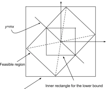
We derive upper and lower bounds on the capacity using this new formulation. We obtain the lower bound by looking for a smaller feasible region inside the parallelogram, i.e., we consider a rectangle inside, and we compute the corresponding mutual information between the input and output with the channel input vector constrained to be inside this rectangular region. For the upper bound, we follow a similar approach, i.e., we look for the the smallest rectangle that inscribes the parallelogram. This geometrical interpretation of the approach is illustrated in Fig. 1.
Fig. 1. The actual feasible region and a smaller region represents the lower bound and an outer region represent the upper bound.
In both the lower and upper bounds, we choose to replace the feasible region with a rectangular one as the rectangular feasible region enables us to separate the two-dimensional problem into two one-dimensional problems whose solutions are readily available.
1) An Upper Bound on the Capacity of 2 × 2 MIMO Systems: A capacity upper bound is derived by solving the
capacity optimization problem over the smallest rectangle that inscribes the original feasible region. This rectangle is constructed from the intersection points of every pair of lines forming the feasible region. The first intersection point is
x= bc d− bAx2− ad d− bAx1, y= c d− bAx2− a d− bAx1,
the second point is x= − bc d− bAx2− ad d− bAx1, y= − c d− bAx2− a d− bAx1,
the third point is x= bc d− bAx2+ ad d− bAx1, y= c d− bAx2+ a d− bAx1,
and the forth point is x= − bc d− bAx2+ ad d− bAx1, y= − c d− bAx2+ a d− bAx1.
Using the geometric interpretation of the feasible region, it is easy to show that in the equivalent formulation of the 2 × 2 MIMO system, the new amplitude limits on the two inputs
∆xupp = " " " " bc d− bAx2 " " " " + " " " " ad d− bAx1 " " " " , (7) ∆yupp= " " " " c d− bAx2 " " " " + " " " " a d− bAx1 " " " " , (8)
can be used to compute an upper bound on the channel capacity of the original MIMO system. Namely, the upper bound of the channel capacity is given by
C≤ C0(∆xupp) + C0(∆yupp), (9)
where C0(A) is the capacity of the point-to-point AWGN
channel for a given amplitude constraint A (computed using Smith’s approach).
2) A Lower Bound on the Capacity of MIMO Systems: A
lower bound on the capacity of the channel can be found by optimizing the mutual information over a smaller rectangular region inside the feasible region (parallelogram). To find such a rectangle, we determine the intersection of a straight line, y = mx, that passes through the origin (as the region is centered at the origin) and the boundary of the feasible region. In this case, it is easy to show that
∆xlow= min !" " " " aAx1 1 + bm " " " " , " " " " aAx1 1 − bm " " " " , " " " " cAx2 1 + dm " " " " , " " " " cAx2 1 − dm " " " " # , (10) ∆ylow= min !" " " " amAx1 1 + bm " " " " , " " " " amAx1 1 − bm " " " " , " " " " cmAx2 1 + dm " " " " , " " " " cmAx2 1 − dm " " " " # , (11) for some arbitrary values for the slope m such that the set of points
{(l∆xlow, k∆ylow) ∈ R : l, k ∈ {1, −1}} ,
where R is the feasible region. Thus, the lower bound on the channel capacity is given by
C≥ C0(∆xlow) + C0(∆ylow). (12)
C. Bounds on the Capacity of General MIMO Systems
For the case of MIMO systems with larger number of transmit and receive elements, a similar approach can be followed to derive upper and lower bounds on the capacity of the channel with amplitude constraints. However, the feasible region of the capacity optimization problem will not be a simple rectangle in the two-dimensional space as in the case of 2 × 2 systems. In other words, although numerical methods can be used to compute the resulting upper and lower bounds on the channel capacity for different noise levels, closed form expressions may not be easy to obtain.
D. Capacity of 2 × 2 MIMO Systems with Amplitude-Limited and Power-Limited Inputs
Smith in [1] showed that for any amplitude-limited and power-limited point-to-point Gaussian channel, a unique capacity-achieving distribution exists and it is discrete. Again, extending these results to the case of MIMO systems is not feasible since there is no result corresponding to the Identity Theorem used in Smith’s proof for multi-dimensional functions. However, we can follow a similar procedure to find upper and lower bounds on the capacity of MIMO systems with amplitude-limited inputs by relaxing the constraint on the amplitude and solving the capacity optimization problem over rectangular regions that inscribe and are inscribed by the original feasible region, respectively. We do not pursue this problem formulation any further in this work.
IV. ASYMPTOTICBOUNDS ON THECAPACITY OF THE 2 × 2 MIMO SYSTEMS
In this section we study the asymptotic behavior of the upper and lower bounds on the capacity of MIMO systems at very high and low noise levels.
A. Very Low Noise Levels
For the point-to-point scalar Gaussian channel for very low noise variances, the entropy of the noise is very small compared to the entropy of the input. Thus, the following approximations are valid,
h(y) ≫ h(y|x) and h(x) ≫ h(x|y). As a result,
h(x) = I(x; y) + h(x|y) = h(y) − h(y|x) + h(x|y) ≈ h(y). That is, the capacity can be approximated as
C = max I(x; y), ≈ max h(x) − h(y|x), = log(2A) −1
2log(2πeσ
2).
Therefore, the capacity of the 2 × 2 MIMO system can be upper and lower bounded for low noise variances as
C≤ log(4∆xupp∆yupp) −
1 2log(2πeσ 2 1) − 1 2log(2πeσ 2 2), (13) C≥ log(4∆xlow∆ylow) −
1 2log(2πeσ 2 1) − 1 2log(2πeσ 2 2). (14) The lower bound on the capacity can be optimized by choosing the slope m (as defined in the previous section) that maximizes the mutual information between the input and the output. We have
C ≥ max
m log (4 |∆xlow∆ylow|)
−1 2log(2πeσ 2 1) − 1 2log(2πeσ 2 2), (15)
such that the set of points
{(l∆xlow, k∆ylow) ∈ R : l, k ∈ {1, −1}} ,
where ∆xlow, ∆ylow, and R are as defined in the previous
section.
B. Very High Noise Levels
For very high noise variances, the optimal distribution is discrete and consists of only two mass points with the same probability [9]. The capacity of this discrete-time binary-input AWGN is well known [10], and the upper and lower bounds on the capacity are
C≤ g# ∆xupp σ1 $ + g# ∆yupp σ2 $ , (16) C≥ g# ∆xlow σ1 $ + g# ∆ylow σ2 $ , (17) where g(x) = 1 −%∞ −∞ 1 √ 2πe− (u−x)2 2 log 2&1 + e−2ux ' du.
C. The Gap Between the Upper and Lower Bounds
For very low noise variances, it is easy to see that the gap between the upper and lower bounds does not depend on the amplitude constraint if Ax1 = Ax2. From (7) and (8), and if
Ax1 = Ax2 = A0 we have,
∆xupp = GuppA0, ∆yupp= HuppA0,
where Gupp and Hupp are only function of the channel
coefficients. Also from (10) and (11),
∆xlow = GlowA0, ∆yupp = HlowA0,
where Glow and Hlow are only functions of the channel
coefficients.
Thus, the gap between the upper and lower bounds ∆C can be written as
∆C = log&4GuppHuppA02' − log &4GlowHlowA20' ,
= log# GuppHupp GlowHlow
$ ,
which is independent of the amplitude constraints imposed on the inputs.
V. NUMERICALEXAMPLES
In this section, we present numerical examples that show the upper and lower bounds for different channel coefficient matrices and different amplitude constraints. For the given channel coefficient matrices and amplitude constraints we use the results of the previous section to come up with new rectangular regions for the channel inputs, and then we numerically evaluate the mutual information as
I( ˜y1,y˜2; ˜x1,x˜2) = I( ˜y1; ˜x1) + I( ˜y2; ˜x2),
= h( ˜y1) + h( ˜y2) − D1− D2,
where h(!) is the differential entropy, and Di= 12log(2πeσi2)
is the entropy of the Gaussian noise with variance equals to σi2, i = 1, 2.
We consider two arbitrarily picked channel matrices given by H1= ( 0.177 0.28 1 0.31 ) , H2= ( 0.997 0.295 1 0.232 ) . We assume that the amplitude constraints imposed on the inputs are identical, and both channels have the same noise variances.
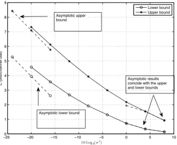
Fig. 2 and Fig. 3 show the upper and lower bounds on the capacity and their asymptotic behavior for the two channels considered. The gap between the upper and lower bounds indicate that there is more work to be done for a tighter characterization of the MIMO channel capacity with amplitude constraints. We also observe that the asymptotic characterizations of the bounds are tight. Fig. 4 shows the upper and lower bounds on the capacity of the second channel for different values of amplitude constraints. Clearly, when the amplitude constraint is increased, the capacity upper and lower bounds are also increased. Also, we observe that the
−250 −20 −15 −10 −5 0 5 10 1 2 3 4 5 6 7 8 9 10 l og1 0( σ2) C (bits/channel use) Lower bound Upper bound Asymptotic upper bound Asymptotic lower bound Asymptotic results coincide with the upper and lower bounds
Fig. 2. Upper and lower bounds on the capacity for H1, along with the asymptotic capacity at low and high noise variances, with an amplitude constraint of 2 (for both inputs).
−250 −20 −15 −10 −5 0 5 10 1 2 3 4 5 6 7 8 9 10 l og1 0( σ2) C (bits/channel use) Lower bound Upper bound
Asymptotic lower bound
Asymptotic results coincide with the upper and lower bounds Asymptotic upper
bound
Fig. 3. Upper and lower bounds on the capacity for H2, along with the asymptotic capacity at low and high noise variances, with an amplitude constraint of 2 (for both inputs).
gap between the upper and lower bounds does not depend on the amplitude constraint for very low noise variance values given that the same amplitude constraints are imposed on both antenna elements. As the value of the noise variance increases, i.e., the SNR decreases, the gap between the upper and lower bound decreases as the number of mass points for the optimal input distribution decreases (eventually it converges to only two mass points).
VI. CONCLUSIONS
We studied the capacity of multi-antenna AWGN channels with amplitude-limited inputs. We computed the capacity of
−150 −10 −5 0 5 10 15 1 2 3 4 5 6 7 10 l og1 0( σ2) C (bits/channel use)
Lower bound, A=2 Upper bound, A=2 Lower bound, A=3 Upper bound, A=3 Upper bound, A=4 Lower bound, A=4
Fig. 4. Illustration of capacity upper and lower bounds of the capacity of H2 for different amplitude constraints on the inputs.
MISO systems using the direct approach proposed by Smith. We derived upper and lower bounds on the capacity of 2 × 2 MIMO systems and characterized their asymptotic behavior. We also illustrated the results using numerical examples.
REFERENCES
[1] J. G. Smith, “The information capacity of amplitude and variance-constrained scalar Gaussian channels,” Information and Control, vol. 18, no. 3, pp. 203–219, 1971.
[2] A. Tchamkerten, “On the discreteness of capacity-achieving distribu-tions,” IEEE Transactions on Information Theory, vol. 50, no. 11, pp. 2773–2778, Nov. 2004.
[3] S. Shamai and I. Bar-David, “The capacity of average and peak-power-limited quadrature Gaussian channels,” IEEE Transactions on
Information Theory, vol. 41, no. 4, pp. 1060–1071, July 1995.
[4] I. C. Abou-Faycal, M. D. Trott, and S. Shamai, “The capacity of discrete-time memoryless Rayleigh-fading channels,” IEEE Transactions
on Information Theory, vol. 47, no. 4, pp. 1290–1301, May 2001.
[5] M. Katz and S. Shamai, “On the capacity-achieving distribution of the discrete-time noncoherent and partially coherent AWGN channels,”
IEEE Transactions on Information Theory, vol. 50, no. 10, pp. 2257–
2270, June 2004.
[6] M. C. Gursoy, H. V. Poor, and S. Verd´u, “The noncoherent Rician fading channel-part I: structure of the capacity-achieving input,” IEEE
Transactions on Wireless Communications, vol. 4, no. 5, pp. 2193–2206,
Sep. 2005.
[7] B. Mamandipoor, K. Moshksar, and A. K. Khandani, “On the sum-capacity of Gaussian MAC with peak constraint,” in IEEE International
Symposium on Information Theory Proceedings, July 2012, pp. 26–30.
[8] O. Ozel and S. Ulukus, “On the capacity region of the Gaussian MAC with batteryless energy harvesting transmitters,” in IEEE Global
Communications Conference, Dec. 2012, pp. 2385–2390.
[9] M. Raginsky, “On the information capacity of Gaussian channels un-der small peak power constraints,” in Annual Allerton Conference on
Communication, Control, and Computing, Sep. 2008, pp. 286–293.
[10] T. M. Duman and A. Ghrayeb, Coding for MIMO Communication