Image super-resolution using deep feedforward neural networks in spectral domain

(1)

IMAGE SUPER-RESOLUTION USING DEEP

FEEDFORWARD NEURAL NETWORKS IN

SPECTRAL DOMAIN

a thesis submitted to

the graduate school of engineering and science

of bilkent university

in partial fulfillment of the requirements for

the degree of

master of science

in

computer engineering

By

Onur Aydın

March 2018

(2)

Image Super-Resolution Using Deep Feedforward Neural Networks In Spectral Domain

By Onur Aydın March 2018

We certify that we have read this thesis and that in our opinion it is fully adequate, in scope and in quality, as a thesis for the degree of Master of Science.

Selim Aksoy(Advisor)

Ramazan G¨okberk Cinbi¸s(Co-Advisor)

Hamdi Dibeklio˘glu

Sinan Kalkan

Approved for the Graduate School of Engineering and Science:

Ezhan Kara¸san

(3)

ABSTRACT

IMAGE SUPER-RESOLUTION USING DEEP

FEEDFORWARD NEURAL NETWORKS IN

SPECTRAL DOMAIN

Onur Aydın

M.S. in Computer Engineering Advisor: Selim Aksoy

Co-Advisor: Ramazan G¨okberk Cinbi¸s March 2018

With recent advances in deep learning area, learning machinery and mainstream approaches in computer vision research have changed dramatically from hard-coded features combined with classifiers to end-to-end trained deep convolutional neural networks (CNN) which give the state-of-the-art results in most of the computer vision research areas. Single-image super-resolution is one of these ar-eas which are considerably influenced by deep learning advancements. Most of the current state-of-the-art methods on super-resolution problem learn a non-linear mapping from low-resolution images to high-resolution images in the spa-tial domain using consecutive convolutional layers in their network architectures. However, these state-of-the-art results are obtained by training a separate neural network architecture for each different scale factor. We propose a novel single-image super-resolution system with the limited number of learning parameters in spectral domain in order to eliminate the necessity to train a separate neural network for each scale factor. As a spectral transform function which converts images from the spatial domain to the frequency domain, discrete cosine trans-form (DCT) which is a variant of discrete Fourier transtrans-form (DFT) is used. In addition, in the post-processing step, an artifact reduction module is added for removing ringing artifacts occurred due to spectral transformations. Even if the peak signal-to-noise ratio (PSNR) measurement of our super-resolution system is lower than current state-of-the-art methods, the spectral domain allows us to develop a single model with a single dataset for any scale factor and relatively obtain better structural similarity index (SSIM) results.

(4)

¨

OZET

SPEKTRAL ALANDA DER˙IN ˙ILER˙I BESLEMEL˙I

S˙IN˙IR A ˘

GLARI KULLANILARAK G ¨

OR ¨

UNT ¨

U S ¨

UPER

C

¸ ¨

OZ ¨

UN ¨

URL ¨

U ˘

G ¨

U

Onur Aydın

Bilgisayar M¨uhendisli˘gi, Y¨uksek Lisans Tez Danı¸smanı: Selim Aksoy

Yardımcı Tez Danı¸smanı: Ramazan G¨okberk Cinbi¸s Mart 2018

Derin ö˘grenme alanındaki son geli¸smelerle birlikte, bilgisayarla görüde ö˘grenme makineleri ve ana yakla¸sımlar, sınıflandırıcılarla birlikte kodlanmı¸s sabit ¨

ozelliklerden u¸ctan uca e˘gitilmi¸s, bilgisayarla görü ara¸stırma alanlarının ¸co˘gunda ba¸sarılı sonu¸clar veren derin evri¸simsel sinir a˘glarına dönü¸smektedir. Tek görüntü süper ¸cözünürlü˘gü, derin ö˘grenme geli¸smelerinden önemli derecede etkilenen alan-lardan biridir. Süper ¸cözünürlük problemindeki mevcut en ba¸sarılı yöntemlerin ¸co˘gu, a˘g mimarilerinde ardı¸sık evri¸simsel katmanları kullanarak uzamsal alanda dü¸sük ¸cözünürlüklü görüntülerden yüksek ¸cözünürlüklü görüntülere do˘grusal ol-mayan bir e¸sle¸stirme ö˘grenirler. Bununla birlikte, bu sonu¸clar, her bir farklı ¨

ol¸cek faktörü i¸cin ayrı bir sinir a˘gı mimarisi e˘gitimi ile elde edilir. Her öl¸cek faktörü i¸cin ayrı bir sinir a˘gının e˘gitilmesinin gereklili˘gini ortadan kaldırmak i¸cin, spektral tanım kümesinde sınırlı sayıda ö˘grenme parametresine sahip yeni bir tek görüntü süper özünürlük sistemi öneriyoruz. Görüntüleri uzamsal tanım kümesinden frekans tanım kümesine dönü¸stüren bir spektral dönü¸süm fonksiy-onu olarak, ayrık Fourier dönü¸sümünün bir varyantı olan ayrık kosinüs dönü¸sümü kullanılır. Buna ek olarak, i¸slem sonrasında, spektral dönü¸sümlerden dolayı mey-dana gelen yapay salınımların kaldırılması i¸cin bir salınım azaltma modülü ek-lenmi¸stir. Süper-¸cözünürlük sistemimizin en yüksek sinyal-gürültü oranı öl¸cümü mevcut ba¸sarılı yöntemlerden daha dü¸sük olsa bile, spektral tanım kümesi, her-hangi bir öl¸cek faktörü i¸cin tek bir veri kümesi ile tek bir model geli¸stirmemizi ve nispeten daha iyi yapısal benzerlik indeksi sonu¸cları elde etmemizi sa˘glar.

(5)

Acknowledgement

First of all, I would like to thank my supervisors, Dr. Selim Aksoy and Dr. R. G¨okberk Cinbi¸s, for their excellent guidance, encouragement, motivation and support during my studies. In addition to their outstanding research contribu-tion, from them, I have learned an effective ’style’ which I could use in every area throughout my life.

I am grateful to my jury members, Dr. Hamdi Dibeklio˘glu and Dr. Sinan Kalkan for kindly accepting to spend their valuable time to review and evaluate my thesis.

Finally, I must express my very profound gratitude to my family and friends for providing support throughout my years of study and through the process of researching and writing this thesis.

Specifically, I would like to express my gratitude to my mother Nihal Aydın for her endless love and my father Nusret Aydın for his enormous power, assis-tance and belief. Additionally, I would like to thank to my sister Burcu Aydın for her life guidance and fellowship, Sezer Aydın for her encouragement, C¸ a˘gla Astarcı for her unlimited support and incredible patience. Finally, I would like to thank to lovely Fındık family members; Eda, Erkut and Eren.

(6)

List of Figures

1.1 An Example of Complete Super-Resolution System . . . 2

2.1 AlexNet Convolutional Neural Network Architecture . . . 10

2.2 SRCNN Network Architecture . . . 14

2.3 Architecture of Deep Laplacian Pyramid Networks . . . 16

2.4 Super Resolution Architecture in Frequency Domain . . . 17

3.1 An Example of Two Dimensional DCT . . . 21

3.2 Two Dimensional Discrete Cosine Transform Basis . . . 22

3.3 Spectral Analysis (x2) . . . 25

3.4 Spectral Analysis Log (x2) . . . 25

3.6 Spectral Analysis Log (x3) . . . 25

(10)

LIST OF FIGURES x

3.9 Bicubic Interpolation . . . 26

3.10 SRCNN . . . 26

3.11 VDSR . . . 26

3.12 LapSRN . . . 26

3.13 SRCNN - First Layer Filters in Spectral Domain . . . 27

3.14 SRCNN - Second Layer Filters in Spectral Domain . . . 28

3.15 SRCNN - Third Layer Filters in Spectral Domain . . . 28

3.16 Most Problematic Frequency Regions . . . 29

3.17 Our Spectral Super Resolution Network . . . 30

3.18 AR-CNN Architecture and Feature Maps . . . 31

3.19 Intermediate Steps of Our Super Resolution System . . . 32

4.1 Set5 Images . . . 34

4.2 Set14 Images . . . 34

4.3 BSDS100 Images . . . 35

4.4 Urban100 Images . . . 35

4.5 Learning Curve for Different Learning Rates . . . 38

4.6 Learning Curve for Different Number of Hidden Units . . . 39

4.7 Learning Curve for PSNR Metric . . . 41

(11)

LIST OF FIGURES xi

4.9 Ours . . . 43

4.10 SRCNN . . . 43

4.11 LapSRN . . . 43

4.12 Output Images of Different SR Models - Set5 1 (x2) . . . 46

A.1 Output Images of Different SR Models - Set5 1 (x2) . . . 61

(12)

LIST OF FIGURES xii

(13)

List of Tables

2.1 The Comparison of Spatial and Frequency Domain SR Models . . 17

4.1 Quantitative Evaluation of SR Models (PSNR - SSIM) . . . 42 4.2 Quantitative Evaluation for Different Setup . . . 44

(14)

Chapter 1 Introduction

This chapter provides a brief overview on single-image super resolution problem. First, a simple definition of the problem is provided, which is followed by a discussion of the main challenges. Then, the scope of our model developed for this thesis is given. At the end, a brief outline of following chapters is provided.

1.1 Overview

The main purpose of the single-image super-resolution (SISR) problem is to re-construct a high-resolution (HR) image from a single low-resolution (LR) image with minimum perceptual resolution loss. From the nature of the problem, super-resolution is an ill-posed inverse problem which searches an inverse function of downsampling and blurring operations. Therefore, in super-resolution problem, there is no unique solution adnd multiple high-resolution image candidates can be produced from a single low-resolution image. Solutions of super-resolution problem might be applied in different areas such as medical imaging, satellite imaging, enlarging consumer photographs, video surveillance, high definition tele-vision broadcasting and so on.

(15)

Figure 1.1: An Example of Complete Super-Resolution System

The single image suresolution problem can be conceptualized from two per-spectives. From signal processing perspective, super resolution problem is a kind of interpolation problem which could be considered as filling intermediate pixel values. From machine learning perspective, super-resolution problem is a kind of regression problem which looks for a continuous mapping from low-resolution im-ages to high resolution imim-ages. Prior to the development of recent deep learning approaches, traditional machine learning techniques such as local linear regres-sion [1, 2], dictionary learning [3, 4] and random forests [5] were being utilized in the supervised resolution approaches. Recently, deep learning based approaches have lead to significant improvements in the state-of-the-art models by learning an effective nonlinear mapping from the LR images to the HR images [6, 7, 8]. There are predominantly two ways for utilizing deep learning techniques in state-of-the-art super-resolution models. First, in the pre-processing step, most single-image super-resolution systems begin with re-sizing input single-images to intended dimensions using bicubic interpolation, which is one of the interpolation tech-niques in the literature. Then, the super-resolution problem reduces to learning a non-linear mapping for transforming the simple interpolation output to a realis-tic high-resolution image as shown in Figure 1.1. However, due to computational complexities and bias of the interpolation technique, in some super-resolution models, it is not preferable to use bicubic interpolation in pre-processing step. Rather, both dimensions and resolution of the images are increased during the

(16)

super-resolution construction. Moreover, while some methods progressively in-crease the resolution of the image, others explore learning a direct non-linear mapping from low-resolution images to high-resolution images. All of the ap-proaches have some advantages and disadvantages based on some criteria.

In SISR problem, there are a few significant points which an SR model must satisfy. The first one is precision which indicates how close an SR model pre-dicts the high-resolution image from its low-resolution counterpart image with minimum loss. Generally, in order to measure the difference between two images in the literature, peak signal-to-noise ratio (PSNR) or the structural similarity index (SSIM) are used. Besides the accurate recovery capability of the model, efficiency is another significant concern of SR problem. Especially due to practi-cal reasons, at test time, the model must work fast and have a low computational cost. Another technical concern is flexibility of the scale factor. The scale factor is a constant that shows how much an image will grow and training a different model for each scale factor is extremely costly and not efficient. Additionally, as scale factor increases, learning a realistic mapping from low-resolution images to high-resolution images becomes harder. Hence, possible short-cut solutions such as first up-sampling with higher scale factor and then down-sampling to intended dimensions would fail rather than learning a scale factor-specific super-resolution mapping. For these reasons, it is preferable to develop a single model for any scale factor. It is expected from any super-resolution model to satisfy all these features and in the literature, different approaches have been developing for each.

1.2 Scope of the Thesis

In this thesis, we developed a new super-resolution model in the frequency do-main with low model complexity. In previous works, convolution neural networks are trained on frequency domain for some specific tasks. For example, Rippel et al. show that convolutional neural networks successfully learn how to classify images completely in Fourier domain [9]. Specifically, discrete cosine transform

(17)

is used to compress weights of convolutional neural networks by protecting pre-diction performance [10]. In another work by Kumar et al, it is indicated that wavelet transforms together with convolutional neural networks generate more successful results than spatial domain methods for single image super resolution problem [11]. In a very recent paper, a super-resolution model is developed in Fourier domain and a novel non-linear activation function is learned to be used in frequency domain [12].

In this thesis, we explore the use of frequency-domain deep neural networks for the single-image super-resolution problem. In our approach, firstly, a non-linear mapping from bicubic interpolated images to high resolution images using deep feed-forward networks is learned completely in frequency domain. Then, in spa-tial domain, a pre-trained artifact reduction network is used to remove resultant frequency artifacts due to frequency domain transforms. We comprehensively evaluate our approach on benchmark datasets and discuss its advantages and disadvantages. Our model provides us a fast and efficient model to remove the necessity to train a different model for each scale factor where a single model would be able to do super resolution on any intended scale factor.

1.3 Outline of the Thesis

In Chapter 2, the necessary technical background on machine learning and the related work on single-image super-resolution problem is provided. In Chapter 3, the details of the proposed model on single image super-resolution problem is given. Additionally, the usage of ringing artifact reduction model in post-processing step is mentioned. In Chapter 4, experiments and results of the proposed model are compared with other state-of-the-art single image super-resolution models. In Chapter 5, conclusions of this study are proposed and possible future work are discussed.

(18)

Chapter 2 Related Work

This chapter provides the necessary technical background on machine learning and the related work on single-image super-resolution problem. In the first part, introductory machine learning definitions and techniques are mentioned. In the second part, fundamental neural network and deep learning techniques from feed-forward neural networks to convolutional neural networks are introduced in detail. In the third part, both traditional and deep learning state of the art approaches on single-image super-resolution problem are provided.

2.1 Machine Learning Background

Machine learning gives computers the ability to learn without being explicitly programmed. A computer program is considered to be learning if it improves its performance on future tasks after making observations about the world. There are different reasons why we want our program to learn. First of all, it is not pos-sible to get rid of all situations that program may encounter during the runtime and it is hard to detect possible changes over time using traditional programming techniques. Additionally, sometimes, it is impossible to find a solution to solve a specific problem. For example, the human brain is great at recognizing objects,

(19)

but it is considered highly difficult to construct a computer program to do the equivalent, without using learning algorithms. For these reasons, it is a must to make computers to learn a good generalization from data or environment to solve many real-world problems. Machine learning can be categorized into three broad classes, depending on the characteristics of the data and the problem.

Supervised Learning: For given input-output example pairs, the definition of the supervised learning is learning a mapping function from input space to output space [13]. Generally, input space might be a feature vector or unstruc-tured raw data such as image or text and output space might be a set of discrete class labels in classification problem or a set of continuous real numbers in re-gression problem. Single-image super-resolution problem is a kind of supervised learning, since the main aim is learning a mapping from continuous low-resolution images to continuous high-resolution images.

Unsupervised Learning: Unlike supervised learning, unsupervised learning algorithms use only input data without any output label and try to find a struc-ture in the data on its own. There are different unsupervised learning algorithms which only use unlabeled data, such as clustering algorithms, autoencoders, and generative adversarial networks [13].

Reinforcement Learning: In the context of reinforcement learning, an au-tonomous agent must learn to perform a task by trial and error, without any guidance. The agent learns from a series of reinforcements, rewards or pun-ishments [13]. Currently, reinforcement learning system based applications are capable to reach human-level performance on many tasks [14] and profoundly increased the performance in the robotics area [15].

According to problem and data type, more problem types are available in machine learning literature such as semi-supervised learning, weakly supervised learning, active learning, one-shot learning, zero-shot learning and so on [13].

(20)

2.2 Deep Learning Background

Deep learning allows computational models to learn representations of data with multiple levels of abstraction. These methods have dramatically improved the state-of-the-art in speech recognition, visual object recognition, object detection and many other domains. Deep learning discovers complex structures in large datasets by using the back propagation algorithm to indicate how a machine should change its internal parameters that are used to compute the representa-tion in each layer from the representarepresenta-tion in the previous layer [16].

Modern deep learning provides a powerful framework for supervised learning. By adding more layers and more units within a layer, a deep network can repre-sent functions of increasing complexity. Most tasks that consist of mapping an input vector to an output vector, and that are easy for a person to do rapidly, can be accomplished via deep learning, given sufficiently large models and sufficiently large data sets of labeled training examples [17].

2.2.1 Introduction to Neural Networks

Artificial neural networks have been inspired by discoveries in neuroscience, par-ticularly from the theory that mental activity principally consists of electrochem-ical signals in a network, called neurons. The neurons in the biologelectrochem-ical network are fired when a linear combination of its inputs surpasses a specific hard or soft threshold. The neurons are associated with neurotransmitters and the neural connections are the ones transporting the electrochemical signals. In the arti-ficial neural network, the neurotransmitters can be considered as weights and the neurons as activation functions. The neural network consist of a collection of nodes that are connected together into a network and the properties of the network are determined by its topology and the properties of each node in the network [17].

(21)

Mathematically, a neuron is modeled as Equation 2.1. xi is the input value,

wij is the corresponding weight for the connection from ith neuron to jth neuron,

bj is the corresponding bias unit and f is the nonlinear activation function. In the

literature, in order to train deep networks effectively, there are various activation functions such as sigmoid, hyperbolic tangent, rectified linear unit (RELU) [18], exponential linear unit (ELU) [19] and so on.

yj = f (

X

i∈I

xiwi,j+ bj) (2.1)

The main target of neural network learning systems is the finding the optimal weights and bias units to minimize problem-specific loss function. In order to minimize loss function, the training samples are passed through the network and the network output is compared with the actual output. The resulting error is used to update the weights of the neurons such that the loss function decreases gradually. This is done using the backpropagation algorithm [20] [21]. Iteratively passing batches of data through the network and updating the weights, so that the loss function is decreased, is an optimization problem. Stochastic gradient descent (SGD), AdaGrad, RMSProp, Adam are some of the main optimization algorithms used to train deep neural networks [22].

2.2.2 Feedforward Neural Networks

Feedforward neural networks form the basis of many significant neural networks being used in the recent times, such as convolutional neural networks (CNN) and recurrent neural networks (RNN). Feedforward neural networks are a kind of di-rected acyclic graph which means that there are no feedback connections or loops in the network. Generally, these networks are known by multiple names such as vanilla neural network, multilayer perceptron, or fully connected networks. Single layer neural network without any activation function is capable to learn a linear function (y = xW ) and this network corresponds to linear regression problem. If an activation function is added to output nodes of this network, a lo-gistic regression model, which is also a linear classification method (y = f (xW )),

(22)

is learned from this network. Since two networks learn a linear function, the problem of finding the best weight parameters turns to a concave optimization problem and only one local minimum point occurs in function space. For this rea-son, optimizing linear networks are relatively easier than deeper networks [17]. On the other hand, if at least one hidden layer is added to the network, the optimization problem turns to a convex problem and function space has multi-ple local minimum points. Therefore, due to convergence to the local minimum problem, optimizing the network turns to a harder problem. Although the diffi-culty of the training, multilayer networks are capable to learn nonlinear functions y = f (f (xW1)W2) that increase the performance of the applications [17].

2.2.3 Convolutional Neural Networks

Convolutional neural networks are very similar to feedforward neural networks. They are made up of neurons that have learnable weights and biases. Each neu-ron receives some inputs, performs a dot product and optionally follows it with a non-linearity. The whole network still expresses a single differentiable score func-tion. And they still have a loss function and all the training and optimization techniques for learning feedforward neural networks still apply.

One of the drawbacks of the feedforward neural networks is that the number of learnable weights dramatically increases as input dimension increases. Clearly, this full connectivity is wasteful and these parameters would quickly lead to over-fitting. By convolution operation, convolutional neural networks look local con-nectivities and vastly reduce the number of parameters and make the forward function more efficiently compared to feedforward neural networks.

In the literature, there are dozens of convolutional neural network architectures for different tasks in various domains such as computer vision, natural language processing, speech recognition and so on. LeNet [21] is the first successful ap-plication of convolutional nets developed in 90s and AlexNet [23] is the network popularized convolutional networks in computer vision. AlexNet is the standard

(23)

convolutional network in the literature and the other popular architectures are derived from this network such as GoogLeNet [24], VGGNet [25] and ResNet [26]. In AlexNet architecture which is shown in Figure 2.1, four different layers are stacked consecutively. The first type of layer is convolution layer which per-forms the convolution operation on input image/activation. This layer computes a dot product between local regions in the input and learned weights on the cor-responding kernel and determines the values of local regions in the output. The second type of layer is activation or RELU layer. This layer applies an element-wise activation function overall activation map. In order to ensure non-linearity of network, a non-linear activation function must be used. Otherwise, even if mul-tiple layers are used, the network is only able to learn a linear function. In the standard architecture, rectified linear units (RELU) activation function is used. The third type of layer is pooling layer. This layer down-samples the activation map along spatial dimension. In the standard architecture, max pooling opera-tion is used. Simply, in max pooling operaopera-tion, highest activaopera-tion map passed through this layer. Finally, the fourth type of layer is fully connected layer. After passing multiple convolution, RELU and pooling layers, an N-dimensional feature vector occurs at the end. Finally, this feature is classified using a dense feedforward neural network. Due to every node is connected to each other, this layer called fully connected layer in deep learning area. Additionally, in order to decrease the overfitting on fully connected layers, dropout regularization tech-nique is used. In overall architecture, convolution, RELU, and pooling layers are responsible for feature extraction part and fully connected layer is responsible for classifying extracted features from previous layers [27].

(24)

2.2.4 Generative Adversarial Networks

Generative adversarial networks (GAN) are neural networks which learn to create artificial data similar to a set of input data. In generative adversarial networks, there two different neural architectures trained simultaneously. The first network (generator network) is trained for learning a mapping to generate artificial ex-amples from latent noise. The second network (discriminator network) is trained for discriminating generated artificial data from real data. In other words, the discriminator network is just a binary classifier which says whether the input is fake or not [28, 29].

min

G maxD V (D, G) = Ex∼pdata(x)[logD(x)] + Ez∼pz(z)[log(1 − D(G(x)))] (2.2)

Since both networks are trained simultaneously, two different optimizers and two different loss functions (generative loss and discriminative loss) are used. Both networks are trained competitively such that while generator network intends to generate realistic indistinguishable samples, discriminator network differentiates real samples from artificial ones. This method of training a generative adversarial network is taken from game theory called the minimax game [28].

2.2.5 Transfer Learning

Traditional machine learning algorithms work under the assumption that there is sufficient number of labeled data for the related problem domain and models fail down when there is not enough data. In other words, for each task and domain, a different model has to be trained with available data. However, in deep learning era, transfer learning provides us to develop a system with small number of samples by transferring knowledge from one domain to another. For example, it is possible to do an MRI image classification system by transferring pre-trained weights of a convolutional neural network classifier which is trained with millions of real world photos. By transfer learning, for every separate task, the necessity to train deep networks from scratch is removed [30, 31].

(25)

2.3 Related Work on Super-Resolution

2.3.1 Traditional Methods

In this part, traditional methods on single-image super-resolution problem are in-troduced. These methods use traditional signal processing and machine learning techniques to increase the resolution of images.

Nearest Neighbor Interpolation

The nearest neighbor interpolation assigns the unknown pixel to the value of nearest pixel point and does not consider other pixels. This is the simplest and piecewise-constant interpolation technique in the literature.

Bilinear Interpolation

Bilinear interpolation assigns the unknown pixel value by fitting a linear curve to nearest four neighbors (2x2) and predict the value on the calculated curve. Bilinear interpolation is smoother than nearest neighbor interpolation.

Bicubic Interpolation

Bicubic interpolation is one of the widely used traditional interpolation methods because of its simplicity and accuracy. Additionally, it is widely used in most super-resolution models in pre-processing step and comparing models. Bicubic interpolation finds the unknown pixel by fitting a polynomial curve to nearest sixteen neighbors (4x4) and predict the value on the calculated curve. Bicubic interpolation is the smoothest interpolation technique among bilinear and nearest neighbor interpolation.

Adjusted Anchored Neighborhood Regression (A+)

Adjusted anchored neighborhood regression for fast super-resolution method is dictionary based SR method which learns a regression model from low resolution to high resolution over dictionaries. In dictionary-based regression model, l2norm

(26)

Random Forest Super-Resolution (RFL)

RFL super-resolution uses random forests to learn a direct non-linear mapping from low-resolution to high-resolution [5]. Random forest regression gives very close results to locally linear regression and a regularization technique is devel-oped for both input and output space.

Self-Similarity Super-Resolution (SelfExSR)

Self-similarity super-resolution method increases the size of internal dictionary size by using geometric transformations and no external dictionary is used. In order to handle perspective distortion and local shape deformation, geometric patch transformation is decomposed [32].

2.3.2 Deep Learning Methods

In this part, deep learning approaches on single-image super-resolution problem are introduced. In recent years, deep learning methods exceed the performance of state-of-the-art methods in many computer vision problems. Super-resolution problem has also been affected positively by recent deep learning advancements.

Super-Resolution Convolutional Neural Network (SRCNN)

SRCNN is the first and simplest deep learning architecture which uses a 3-layered convolutional neural network, for single-image super-resolution problem. Cur-rently, it is the benchmark model for our development and each SR model which uses deep learning approach. Even if the performance of SRCNN model is ex-ceeded currently, due to its simplicity and speed, SRCNN is still a valuable ar-chitecture in SR problem for comparing models.

In SRCNN (Figure 2.2), after applying bicubic interpolation in preprocessing step, the image is passed through three consecutive convolution layers. As stated in the paper, the operation in the first convolution layer is the patch extraction and representation layer, the second layer performs a nonlinear mapping oper-ation and the third convolutional layer is the final layer which reconstructs the

(27)

Figure 2.2: SRCNN Network Architecture [6]

high resolution image from activations of the second convolutional layer. At the end, high resolution image is recovered by using three consecutive convolution layers.

During the optimization of the network, l2 loss function is minimized using

stochastic gradient descent optimizer. Additionally, output high resolution image is reconstructed directly. One drawback of the SRCNN model is that for each scaling factor, a separate model is trained. On the other hand, SRCNN provides the flexibility that with larger datasets and deeper architectures, the SR perfor-mance might be outperformed [6].

Faster Super-Resolution Convolutional Neural Network (FSRCNN) Differing from SRCNN that uses bicubic interpolation in preprocessing step, FSR-CNN introduces a deconvolution layer at the end of the network and the mapping is learned directly from the original low-resolution image. This architecture pro-vides us to learn deeper convolutional layers with lower computational cost. In the architecture of FSRCNN, seven convolutional layers and one deconvolu-tional layer is used and architecture is divided into five different regions according to their task such that feature extraction, shrinking, mapping, expanding and de-convolution. Like SRCNN, during the optimization, l2 loss function is minimized

and as an optimizer stochastic gradient descent is used. Additionally, direct high resolution image reconstruction is performed [33].

(28)

Very Deep Super Resolution (VDSR)

Unlike SRCNN architecture which uses only 3 convolutional layers, VDSR stacks 20 convolutional layers. In other words, VDSR is the deeper version of SRCNN ar-chitecture. Furthermore, VDSR added a residual connection from the input layer to output layer in order to solve the vanishing gradients problem while training deep networks. Differing from SRCNN, VDSR uses ten times higher learning rate and due to scale augmentation technique, only one network is trained for all scaling factors rather than training a separate network [7].

Super-Resolution Generative Adverserial Networks (SRGAN)

In SRGAN model, super resolution network is trained in adversarial setting. The generator learns to generate an HR image from input LR image. On the other hand, the discriminator network learns to discriminate generated super-resolved image and original high resolution image. Both networks are trained end-to-end in adversarial setting. The SRGAN method optimizes the network using the per-ceptual loss and the adversarial loss for photo-realistic SR [34].

Laplacian Super-Resolution Networks (LapSRN)

Unlike SRCNN, in LapSRN, no interpolation step is used during preprocessing step. Instead, the dimensions are progressively increased using Laplacian pyra-mid framework using 27 convolutional layers as shown in Figure 2.3. Additionally, residual connections are used in the architecture. During optimization, instead of l2 loss function, Charbonnier loss function is used which is a robust loss function

to handle outliers and more proper to the human visual perception.

The model presented in that paper consists of two parts such that feature ex-traction and image reconstruction. Transpose convolutional layer connects to two different layers. First is reconstruction layer and the other one is the convo-lutional layer that represents better resolutions. Contrary to other networks that are mentioned, the network designed in that paper has a less complex feature extraction. Because feature extraction is shared between lower and higher levels and complex mappings can be learned by this network better. During image reconstruction, input images are upscaled with the order of two and transposed

(29)

Figure 2.3: Architecture of Deep Laplacian Pyramid Networks [8]

convolutional layer. Then the pixel-wise sum of residual images from feature ex-traction and the upscaled image is used to produce a HR image as the output [8]. Wavelet Domain Super-Resolution (CNNWSR)

CNNWSR is a super-resolution network which trained for predicting discrete wavelet transform coefficients of target HR image. Then, using the reconstruc-tion power of wavelet transform, the high resolureconstruc-tion image is reconstructed from predicted wavelet coefficients using two-dimensional inverse wavelet transform. In the prediction model of CNNWSR, three convolutional layers are used like SR-CNN architecture, except SRSR-CNN produces one output image while SR-CNNWSR predicts three output images which contain all wavelet coefficients. This is the first architecture combines the deep learning and spectral approaches in super-resolution problem. However, the main problem of the CNNWSR architecture is the scale limitation which stems from the nature of wavelet transform [11].

(30)

Frequency Domain Super Resolution (FourierSR)

In a very recent unpublished work, a Fourier domain approach to super resolu-tion problem is made. In this paper, as shown in Figure 2.4, a deep network is constructed and learned totally in Fourier domain. Additionally, using properties of Fourier transform, such as convolution in the spatial domain is equivalent to multiplication in the frequency domain and vice versa, convolutional layers are treated as multiplications and non-linear activation functions are substituted by convolutions in frequency domain [12].

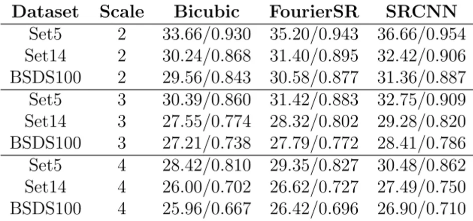
Figure 2.4: Super Resolution Architecture in Frequency Domain [12] Although Fourier transform brings the computational efficiency, the frequency domain is not a proper domain for highly accurate super-resolution. From Table 2.1, it is observed that PSNR and SSIM values (PSNR/SSIM) of super resolution in Fourier domain are relatively lower than spatial domain methods.

Table 2.1: The Comparison of Spatial and Frequency Domain SR Models Dataset Scale Bicubic FourierSR SRCNN

Set5 2 33.66/0.930 35.20/0.943 36.66/0.954 Set14 2 30.24/0.868 31.40/0.895 32.42/0.906 BSDS100 2 29.56/0.843 30.58/0.877 31.36/0.887 Set5 3 30.39/0.860 31.42/0.883 32.75/0.909 Set14 3 27.55/0.774 28.32/0.802 29.28/0.820 BSDS100 3 27.21/0.738 27.79/0.772 28.41/0.786 Set5 4 28.42/0.810 29.35/0.827 30.48/0.862 Set14 4 26.00/0.702 26.62/0.727 27.49/0.750 BSDS100 4 25.96/0.667 26.42/0.696 26.90/0.710

(31)

Chapter 3 Method

In this chapter, the details of our model for single-image super-resolution problem are given. First of all, spectral domain techniques to transform signals from time domain (or spatial domain) to frequency domain are investigated. Then, the usage and contributions of spectral domain techniques in super-resolution problem for our model are given in detail. In the last section, our complete super-resolution system is described in detail. In the initial part of the system, the neural network architecture and learning procedure to learn a mapping from low resolution images to high resolution images are described. At the end, artifact reduction network in post-processing step in order to eliminate spectral ringing artifacts is described.

3.1 Spectral Domain Transforms

In this section, spectral domain transform functions are investigated. Basically, spectral domain transforms the representation of a time (spatial) domain signal to the frequency domain. Two different spectral transforms are investigated in this section such that Fourier transform and its variant, discrete cosine transform which are a quite popular transforms in signal processing domain.

(32)

3.1.1 Fourier Transform

First of all, Fourier transform and its different variants are provided. The basic definition of Fourier Transform is decomposing any differentiable real or complex signal into different complex exponential functions which oscillate at different frequencies. In other words, Fourier Transform converts the representation of a time domain signal to the frequency domain. Fourier Transform provides us to analyze signals in the frequency domain which might be easier than time domain analysis in some situations. However, due to basis functions, Fourier Transform produces complex outputs even if the input is a real signal. For a continuous signal f and its frequency domain representation F, one-dimensional Fourier Transform is defined as follows [35]: F (w) = 1 2π Z ∞ −∞f (x)e −jwx dx (3.1)

Additionally, the signal transformed to the frequency domain is reconstructed back via one-dimensional Inverse Fourier Transform which is defined as follows:

f (x) =

Z ∞

−∞F (w)e jwx

dτ (3.2)

3.1.1.1 1-D Discrete Fourier Transform

Fourier Transform is a complex-valued operation for continuous signals. However, in digital systems, every signal is discrete and things that are valid for continuous signals begin to lose their validity for discrete signals. For this reason, Discrete Fourier Transform (DFT) is specifically designed to be used in digital systems. For a discrete signal f and its frequency domain representation F, one-dimensional Discrete Fourier Transform is defined as follows [35]:

F [u] = 1 M M −1 X x=0 f [x]e−2πj(uxM) (3.3)

The signal transformed to the frequency domain is reconstructed back via one-dimensional Inverse Discrete Fourier Transform which is defined as follows:

f [x] =

M −1

X

(33)

3.1.1.2 2-D Discrete Fourier Transform

Until now, Fourier Transforms for signals in one-dimensional space are mentioned. In this section, Fourier Transforms for two-dimensional discrete signals such as image, video, etc., are introduced. For a two dimensional discrete signal f and its frequency domain representation F, two-dimensional Discrete Fourier Transform is defined as follows [35]: F [u, v] = 1 N M N −1 X x=0 M −1 X y=0 f [x, y]e−2πj(xuN+ yv M) (3.5)

The signal transformed to frequency domain is reconstructed back via two-dimensional Inverse Discrete Fourier Transform which is defined as follows:

f [x, y] = N −1 X u=0 M −1 X v=0 F [u, v]e2πj(xuN+ yv M) (3.6)

3.1.2 Discrete Cosine Transform

In previous section, Fourier Transform and its variants are given in detail. How-ever, even if the input signal is real, Fourier Transforms are complex valued operations which output a complex signal. On the other hand, discrete cosine transform which decomposes a signal into cosine functions which oscillates at different frequencies is a real valued transform and gives a real signal in output.

3.1.2.1 1-D Discrete Cosine Transform

For a one dimensional discrete signal f and its frequency domain representation F, one-dimensional Discrete Cosine Transform is defined as follows [35]:

F [u] = a(u) N −1 X x=0 f [x]cos π(2x + 1)u 2N ! (3.7) The signal transformed to frequency domain is reconstructed back via two-dimensional Inverse Discrete Cosine Transform which is defined as follows:

f [x] =

N −1

X

x=0

a(u)F [u]cos π(2x + 1)u 2N

!

(34)

3.1.2.2 2-D Discrete Cosine Transform

For a two dimensional discrete signal f and its frequency domain representation F, two-dimensional Discrete Cosine Transform is defined as follows [35]:

F [u, v] = a(u)a(v) N −1 X x=0 M −1 X y=0 f [x, y]cos π(2x + 1)u 2N ! cos π(2y + 1)v 2M ! (3.9) The signal transformed to frequency domain is reconstructed back via two-dimensional Inverse Discrete Cosine Transform which is defined as follows:

f [x, y] = N −1 X x=0 M −1 X y=0

a(u)a(v)F [u, v]cos π(2x + 1)u 2N ! cos π(2y + 1)v 2M ! (3.10) Where a(x) is defined as:

a(x) =    q 1 N, x = 0 q 2 N, x 6= 0 (3.11)

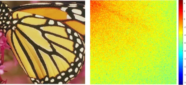
In the Figure 3.1, an example of 2-D DCT of given image is provided. As it is seen, visually, it is impossible to understand what the image is and there is no local correlation among pixel values in spectral domain. Top left corner values represent low, bottom right corner values represent high frequencies.

(35)

Additionally, in the Figure 3.2, the basis functions for two-dimensional discrete cosine transform is provided. Each basis function is a two-dimensional represen-tation of the combination of two cosine functions which are oscillated in different frequencies. As going from top to bottom and left to right, frequencies of cosine functions increase. For this reason, basis functions in the top left corner have lower frequency values and basis functions in the bottom right corner have higher frequency values. The first basis function which is located in top left corner is constant DC term and this basis function consists of all ones. In other words, DC term is equivalent to calculate the mean value of transformed input patch:

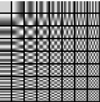
Figure 3.2: Two Dimensional Discrete Cosine Transform Basis

A significant feature of discrete cosine transform is energy compaction property. By this property, DCT preserves considerably more information in low frequen-cies. Discrete cosine transform is the best approximation of Karhunen-Loéve transform which is theoretically ideal linear dimension reduction technique. The principal component analysis is a specific version of Karhunen-Loéve transform and has data dependent basis functions. Constant cosine basis functions of dis-crete cosine transform ideally approximate Karhunen-Loéve transform.

(36)

3.2 The Developed Model

In this part, the details of the developed model, network architectures and their implementations are given. First of all, initial super-resolution model is devel-oped using neural networks in the spectral domain. After super-resolution phase, another network is used in spatial domain in order to decrease ringing artifact effect which is caused by spectral transforms.

3.2.1 Super Resolution in Spectral Domain

In our super-resolution model, firstly, a significant analysis and observation be-tween low-resolution and high-resolution images in spectral domain are made. Additionally, extra observations over different super-resolution models are made in order to compare bicubic interpolation. Then, from these observations, a net-work architecture and learning system is constructed to learn a mapping from low-resolution to high-resolution. In this section, the details of the developed super-resolution model and the architecture are given.

3.2.1.1 Model Development

Before constructing network architecture, an initial data analysis is made in the spectral domain. Most super-resolution problems use bicubic interpolation tech-nique to resize low-resolution images to intended dimensions in pre-processing step. For this reason, this analysis is made between bicubic interpolated images and their high resolution versions. Therefore, it is tried to investigate the exact problem behind bicubic interpolation.

First of all, a low resolution image is resized to intended dimensions using bicu-bic interpolation method (e.g. scale factors of x2, x3, x4). Then, each image is divided into patches with a stride of patch size. Independent of the scale factor, each patch corresponds to 16x16 patch in low resolution version. Hence, patch

(37)

dimensions are 32x32, 48x48 and 64x64 for scale factors 2, 3 and 4 respectively. After generating patches, two-dimensional discrete cosine transform of each patch is computed for both interpolated and high resolution images. In order to observe the weaknesses of bicubic interpolation, the mean square error between bicubic interpolated patches and high resolution patches is calculated and averaged across patches. Finally, results of mean square error analysis in spectral domain is at-tained.

For three different scale factors, the average mean square error calculations are given in Figures 3.3, 3.5 and 3.7 and their logarithmic versions are given in Figures 3.4, 3.6 and 3.8. In these figures, each pixel in images corresponds a frequency value over a 2-dimensional array. Simply, top left corner pixels represent low frequencies, bottom right corner pixels represent high frequencies and remaining regions represent mid-frequencies. From mean square error analysis, it would be said that bicubic interpolation works well (or less problematic) for low and high frequencies, but, the actual problem is in mid-frequencies. However, in most papers, due to problems on edges of super-resolution images, it is blindly stated that SR algorithms fail to predict high frequency terms.

After these observations, we concentrate on fixing this problematic band-pass region in our neural network model. Moreover, for different scale factors, it is ob-served that a common mid-band region is problematic and this common pattern allows us to develop a single model for all scale factors. It is important to state that even current and previous state-of-the-art super resolution methods do not have this property and it is still needed to develop a separate network for each scale factor which brings the requirement of more training duration and more data with different scales. Additionally, during test time, it is required to hold whole network models in memory for every scale factor. For these reasons, it is better to design a super resolution model which fits all scale factors.

(38)

Figure 3.3: Spectral Analysis (x2) Figure 3.4: Spectral Analysis Log (x2)

Figure 3.5: Spectral Analysis (x3) Figure 3.6: Spectral Analysis Log (x3)

(39)

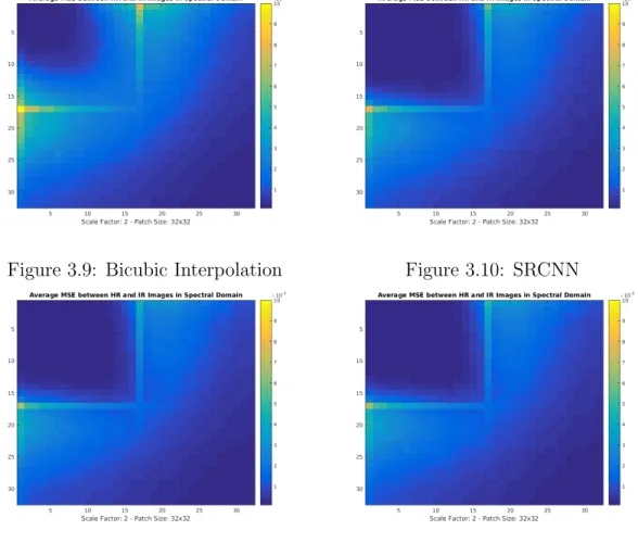
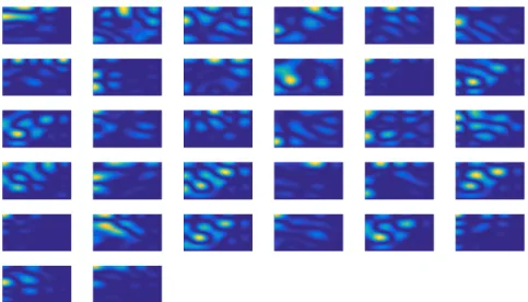
After observing the mean square error between bicubic interpolated and high resolution images in the spectral domain, the same analysis is made for different super resolution models such as SRCNN, VDSR, and LapSRN and it is observed how each SR model fixes low resolution images in the spectral domain. From Figures 3.9, 3.10, 3.11 and 3.12, very similar outputs are obtained with bicubic interpolation except lower frequency values are fixed better. However, there are still some problems in mid-frequency bands. The performance of SR algorithms in sorted ascending order are bicubic interpolation, SRCNN, VDSR and LapSRN and this pattern is also observed in spectral domain quite clearly.

Figure 3.9: Bicubic Interpolation Figure 3.10: SRCNN

Figure 3.11: VDSR Figure 3.12: LapSRN

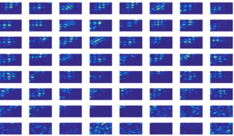
After analyzing different super resolution networks in the spectral domain, as stated in previous section, it is understood that these algorithms are able to re-cover lower frequencies but mid-frequencies are still problematic. After these data input-output analysis, spatial filters learned in SRCNN architecture are analyzed

(40)

in spectral domain in order to understand what SRCNN learns in the spectral domain. SRCNN is three-layered convolutional neural network architecture and in the first layer 64 9x9 filters, in the second layer 32 5x5 filters and in the third layer 32 5x5 filters are available. Additionally, there are different filter size setups are available for SRCNN architecture, but this setup is arbitrarily selected among others.

In the analysis, two-dimensional discrete cosine transform of each spatial filter is taken. Moreover, for better visual quality, 64-point FFT’s are used in two-dimensional DCT calculation. The learned filters in spectral domain are shown in Figures 3.13, 3.14 and 3.15. From filters below, learned filters are generally low pass filters which give more spikes in low-frequency regions. Additionally, even if for some filters, there are a few spikes occur in high and middle frequencies, at the end, these filters are not able to fix these regions.

(41)

Figure 3.14: SRCNN - Second Layer Filters in Spectral Domain

(42)

3.2.1.2 The Network Architecture

The main function of our neural network architecture is learning a mapping from low resolution images to high resolution images so that the problematic region which is discussed in the previous section is fixed. Additionally, the developed net-work must be usable for any scale factor. Therefore, input and output dimensions must be compatible for each scale factor. For these reasons, most 512 erroneous frequency values in mean square error analysis, which is shown in Figure 3.16, are determined and for input and output, these 512 mid-frequency values are used. For scale factor of two, images are divided into 32x32 patches and there are a total of 1024 two dimensional frequency values in the spectral domain. Therefore, half of the patches are included in the learning process.

Figure 3.16: Most Problematic Frequency Regions

For the input to the neural network, the problematic region of bicubic inter-polated patches and for the output to the neural network, the corresponding problematic region of high resolution patches are given. Then, a neural network architecture is trained for minimizing the mean square error between predicted and high resolution versions of the problematic frequencies. In order to learn this mapping, a feedforward fully connected neural network is constructed. Unlike

(43)

the spatial domain, there is no homogeneous distribution between pixel values in the spectral domain. For this reason, fully connected networks are preferred over convolutional neural networks. In the network architecture, a four-layered fully connected neural network is used and in each layer, 512 hidden units are used. Therefore, total of 1050624 parameters are learned in the network architecture. All weights are initialized using Xavier normal initializer [36] and the network is trained using Adam optimizer [22] with the batch size of 128. An overview of our super-resolution system is shown in Figure 3.17.

Figure 3.17: Our Spectral Super Resolution Network

In order to prevent overfitting, after each fully connected layers, dropout layers are placed [37]. Moreover, because discrete cosine transform mostly produces numbers between -1 and 1 (except DC term), the hyperbolic tangent function is used rather than rectified linear unit which is a better choice for vanishing gradients problem [18]. Especially in the output layer, using hyperbolic tangent function allow us to constrain output to be between -1 and 1. Beside all these setups, more optimization techniques, activation function, and training proce-dures are tried such as RMSProp optimizer, SRELU activation function or batch normalization [38], the best performance is obtained using given setup.

(44)

3.2.2 Artifact Reduction in Spatial Domain

After training our spectral super resolution network, some ringing artifacts are ob-served due to used spectral transforms. Since Fourier transform of a rectangular function is sinc function those oscillations approach to infinity, these artifacts are observed when some changes are made in the spectral domain. Because Fourier transform and discrete cosine transform are very similar functions, a similar sit-uation is also valid for DCT. This is a very common problem for many image processing applications. For instance, JPEG compression algorithm uses discrete cosine transform and compression process in spectral domain generates similar artifacts in the spatial domain.

Figure 3.18: AR-CNN Architecture and Feature Maps [39]

Like super resolution problem, deep neural networks are also used to solve com-pression artifact reduction problem. For instance, AR-CNN is the first deep learn-ing architecture to reduce compression artifacts from JPEG images. As shown in Figure 3.18, AR-CNN architecture which uses consecutive convolutional layers is very close to SRCNN super resolution architecture and it is used as a base-line method for artifact reduction problem in the literature [39]. After AR-CNN model, a deeper version of AR-CNN architecture is developed. In this architec-ture, 8 consecutive convolution layers are used and between these convolutional layers, skip connections are added to prevent gradient vanishing problem [40]. After our spectral super resolution model, in order to remove ringing artifacts, a pre-trained model of AR-CNN model is used. Even if the model is not re-trained end-to-end manner, a considerable amount of increase in our super-resolution

(45)

model is obtained. Even if better results would be obtained from our complete super resolution system, we don’t want to end-to-end train a separate network to solve artifact reduction problem. Because, at this time, the problem would turn to learn an SRCNN model in the spatial domain. Additionally, AR-CNN model is trained on a completely different dataset. Therefore, it is more valu-able to transfer the artifact reduction knowledge to super-resolution domain. In conclusion, when complete super resolution system is thought, using spectral transforms in the initial step, super-resolution problem is converted to artifact reduction problem and it is solved using pre-trained artifact reduction neural networks in the spatial domain. In the Figure 3.19, intermediate steps of our complete single-image super-resolution system and increasing of PSNR value in each step is shown.

.

(46)

Chapter 4 Experiments

In this chapter, the details of our experimental setup and completed experiments are given. In the first part, datasets used during experiments both in training and testing phase are mentioned. Then, evaluation metrics for super-resolution problem which are widely used in the literature are described mathematically. Finally, evaluation metrics and output images of experiments done for the devel-oped model is shared.

4.1 Dataset Information

An advantageous of super-resolution problem is that any kind of image data can be used directly in both training and testing phases and unlike some problems like classification, detection or segmentation, no human effort is needed to label images manually. Any image is being both data and label at the same time in super-resolution problem. The original image is taken as high-resolution image or in other words output label. Then, low-resolution image or in other words input data is obtained by down-sampling original high-resolution image. At the end, input data and output label are prepared without any cost using any image dataset. In the following section, details of training and test sets are given.

(47)

4.1.1 Training Sets

In training phase, three different image datasets are used. These are BSDS200, General100, and T91. There are 200, 100 and 91 images in datasets respectively and there are 391 images in total. These are the widely used datasets in the literature for single-image super-resolution problem.

4.1.2 Test Sets

In test phase, four different image datasets, Set5, Set14, BSDS100, and Urban100, are used. These are shown in Figure 4.1, 4.2, 4.3 and 4.4 respectively. There are 5, 14, 100 and 100 images in datasets respectively and there are 219 images in total. Additionally, Set5 dataset is used as development set and it is used for model selection and parameter tuning. Especially Set5 and Set14 datasets are very commonly used in the literature. In the following figures, samples from image datasets are shared for gaining better insight about images.

Figure 4.1: Set5 Images

(48)

Figure 4.3: BSDS100 Images

Figure 4.4: Urban100 Images

4.2 Model Evaluation

In this section, evaluation metrics used in super-resolution problem are math-ematically described. There are two different evaluation metrics used in this thesis. These are Peak Signal-to-Noise Ratio (PSNR) and Structural Similarity Index (SSIM). For super-resolution problem, it is preferable to obtain high PSNR and SSIM values from models. However, high PSNR or SSIM value does not al-ways mean high perceptual quality. For instance, sometimes, it is possible to obtain a high-resolution image from low-resolution with lower PSNR, but higher perceptual quality. For this reason, current evaluation metrics are a bit problem-atic and finding a better evaluation metric for super-resolution problem is still an open research problem. In the following section, mathematical details of peak signal-to-noise ratio (PSNR) and structural similarity index (SSIM) are given.

(49)

4.2.1 Peak Signal-to-Noise Ratio (PSNR)

Peak signal-to-noise ratio is a metric which measures the quality difference be-tween two input images. Theoretically, higher PSNR means higher image quality. For M xN dimensional images I1 and I2, PSNR is described as follows:

P SN R = 10 log₁₀ R 2 M SE ! (4.1) M SE = P M,N[I1(m, n) − I2(m, n))]2 M N (4.2)

In the equation, M SE is the mean square error between two images and R is the maximum range of the input image. For instance, for double precision floating data type, R is equal to 1 and 8-bit unsigned integer data type R is equal to 255. For color images, RGB images are converted to YCbCr color space and PSNR is calculated on luminance channel only due to sensitivity of human eye to luminance channel.

4.2.2 Structural Similarity Index (SSIM)

The Structural Similarity Index (SSIM) quality assessment index is based on the computation of three terms, namely the luminance term, the contrast term and the structural term. The overall index is calculated by multiplying all three terms. For M xN dimensional images I1 and I2, SSIM is described as follows:

SSIM (x, y) = [l(x, y)]α[c(x, y)]β[s(x, y)]γ (4.3)

where l(x, y), c(x, y) and s(x, y) are defined as follows:

l(x, y) = 2µxµy+ C1 µ2

x+ µ2y+ C1

(50)

c(x, y) = 2σxσy+ C2 σ2 x+ σy2+ C2 (4.5) s(x, y) = σxy + C3 σxσy+ C3 (4.6)

where µx, µy, σx, σy and σxy are the local means, standard deviations, and

cross-covariance for images x, y. If α = β = γ = 1 (default values) and C3 = C2/2

(default selection of C3) the index simplifies to:

SSIM (x, y) = (2µxµy + C1)(2σxy+ C2) (µ2

x+ µ2y+ C1)(σx2+ σ2y + C2)

(4.7)

4.3 Super-Resolution Experiments

In this section, experimental details of our super-resolution model are given. For measuring the performance of SR algorithm, peak signal-to-noise ratio (PSNR) and structural similarity index (SSIM) are used as mentioned in the previous section. In this section, our model is compared with other super-resolution models in PSNR and SSIM measurements which are mentioned in previous section.

4.3.1 Optimization Experiments

In this part, experiments on hyperparameters of network optimization and other sub-experiments which fortify the purpose of our model are provided. Initially, it is discussed how different hyperparameter selections affect the performance of the network architecture. In order to optimize the network, using grid search tech-nique, extremely many network and hyperparameter setups are constructed and trained/tested. At the end, the best network architecture and hyperparameter selection are used as final network structure. In this part, results and learning

(51)

curves of a few experiments on selection of important hyperparameters are pro-vided. Additionally, other sub-experiments are provided in order to support the importance of our model.

Learning Rate Experiments

After making a set of experiments, we determined a set of hyperparameters and network architecture design which give the best super-resolution performance. Then, by changing learning rate parameter, it is intended to observe the effect of the change of learning rate on the designed network. For three different learning rate parameters, experiments are completed and learning curves are plotted for training data which is shown in the Figure 4.5. Additionally, for validation data, we obtained very similar learning curves as train data. From learning curves, we observed that with highest learning rate, network converged very rapidly and as learning rate decreases, convergence time of the network increases. Interestingly, all networks with different learning curves are converged to same point and same loss function is obtained with each network (Even if it is not shown in the figure, we observed that with more epochs, yellow line also converged to same point).

(52)

The Number of Hidden Units Experiments

Like learning curve experiments, we selected best hyperparameters and network architecture design which give the best super-resolution performance. Then, by changing the number of hidden units per layers, it is intended to observe the effect of the change of learning rate on the designed network. For three different number of hidden units parameters, experiments are completed and learning curves are plotted for training data which is shown in the Figure 4.6. From learning curves, we observed that even if the convergence time change as increasing number of hidden units, the network converged to same point like learning rate experiments. Additionally, with different number of hidden units combinations in intermediate layers, we obtained very similar results.

(53)

Artifact Reduction Experiment

In order to measure the importance of artifact reduction module after super-resolution network, a set of experiments are made by using different combinations of these modules. In the first set of experiments, three different combinations which are only bicubic interpolation, bicubic interpolation followed by artifact reduction and bicubic interpolation followed by super-resolution and artifact re-duction, are used. Respectively, 33.69 dB, 33.82 dB and 35.53 dB PSNR values are obtained using Set5 test dataset. In other words, even if artifact reduction network is a deep image enhancement technique, just using AR network increases the super-resolution performance only 0.13 dB. In the second set of experiments, similar experiment is made with SRCNN network as a super resolution module. Additionally, an ensemble of our network and SRCNN is used. In all these experi-ments, we obtained lower PSNR values than bicubic interpolation. In conclusion, all these experiments are an indication of consistency of our model.

Artifact Reduction JPEG Quality Experiment

In artifact reduction model, there are four different pre-trained models. Each network is trained with different image sets according to their JPEG compression quality (Q = 10,20,30 and 40). At the end of all four experiments, the network which gives highest PSNR value is used as a final model. Best PSNR value is obtained with Q=40 which is the highest JPEG quality.

4.3.2 Evaluation Results

In Table 4.1, PSNR and SSIM values of ten different super-resolution models are provided. Additionaly, the Figure 4.7 indicates how average PSNR value which is favored by loss function is increased during the training. In experiments, four different test datasets and three scale factors (x2, x3, x4) are used. First of all, bicubic interpolation is the simplest super-resolution technique in the liter-ature and lowest PSNR and SSIM results are obtained from its output images as expected. The measurements of bicubic interpolation is the lower bound for super-resolution problem. From Table 4.1, it would not be wrong to generalize

(54)

that spatial domain super-resolution models are far better models than frequency domain methods and deeper models are more successful than traditional and shal-lower ones. Additionally, increasing the dimension of images progressively gives relatively better results than direct reconstruction methods.

In comparing our model with other super-resolution architectures, it is observed that our super-resolution model is able to give closer results to other state-of-the-art models on SSIM metric rather than PSNR metric. Since in state-of-the-state-of-the-art models, the deep networks are trained for minimizing mean square error loss in spatial domain, this favors to obtain high PSNR results. However, since our model is trained in spectral domain, intended high PSNR values are not obtained. Rather, better SSIM results are obtained. In other words, our model produces images closer to ground truth in statistical manner, not pixel-wise manner.

Image super-resolution using deep feedforward neural networks in spectral domain

IMAGE SUPER-RESOLUTION USING DEEP

FEEDFORWARD NEURAL NETWORKS IN

SPECTRAL DOMAIN

a thesis submitted to

the graduate school of engineering and science

of bilkent university

in partial fulfillment of the requirements for

the degree of

master of science

in

computer engineering

By

Onur Aydın

March 2018

ABSTRACT

IMAGE SUPER-RESOLUTION USING DEEP

FEEDFORWARD NEURAL NETWORKS IN

SPECTRAL DOMAIN

¨

OZET

SPEKTRAL ALANDA DER˙IN ˙ILER˙I BESLEMEL˙I

S˙IN˙IR A ˘

GLARI KULLANILARAK G ¨

OR ¨

UNT ¨

U S ¨

UPER

C

¸ ¨

OZ ¨

UN ¨

URL ¨

U ˘

G ¨

U

Acknowledgement

Contents

List of Figures

List of Tables

Chapter 1

Introduction

1.1

Overview

1.2

Scope of the Thesis

1.3

Outline of the Thesis

Chapter 2

Related Work

2.1

Machine Learning Background

2.2

Deep Learning Background

2.2.1

Introduction to Neural Networks

2.2.2

Feedforward Neural Networks

2.2.3

Convolutional Neural Networks

2.2.4

Generative Adversarial Networks

2.2.5

Transfer Learning

2.3

Related Work on Super-Resolution

2.3.1

Traditional Methods

2.3.2

Deep Learning Methods

Chapter 3

Method

3.1

Spectral Domain Transforms

3.1.1

Fourier Transform

3.1.2

Discrete Cosine Transform

3.2

The Developed Model