Online ECG signal orthogonalization based on singular value decomposition

I l II I 5 й ¡Ç Ä ŞIЩ t î s î Й T y Jî ■ ?! fa 5« ;:¡ a 4 J g -y ? ^ ц W ιί·* -*1 ·ί» ü’·· *^. •i«· '·.>■' ■.■> U «,ν ,iw vu w-i ¿.1 .^ -Λ· ’«■ . . .’ · Г ti. i i!i * -i ч*;· oç

л| ι·4 i f '’V5 .:і^ -'Ч I ¡4 Д' - Хі f '.'і · ι . ■'= -' ! ^ і/’^

¡íti* Oí W «чга '■-%/ ** V Ч*4<^ ^ ц' ^ *Ч>*' Ч U ·* ·Α^ ’•!^' т»** ^ W *·«^ і ¿ ¿.i¿

¿H ¿ /"í XÜ w ^ ~·'ΐ -.Й». Ϊ ^-4. ,1 fj· 1 л*;^ j ■.:':v.c* :A-_{■w¿ » ► .■}d. ТЧ < í P / Í 2 .- 5 ‘ S i ,

1 3 9 6

ONLINE EGG SIGNAL ORTHOGONALIZATION

BASED ON SINGULAR VALUE DECOMPOSITION

A THESIS

SUBMITTED TO THE DEPARTMENT OF ELECTRICAL AND ELECTRONICS ENGINEERING

a n d t h e i n s t i t u t e o f ENGINEERING AND SCIENCES OF BILKENT UNIVERSITY

IN PARTIAL FULFILLMENT OF THE REQUIREMENTS FOR THE DEGREE OF

MASTER OF SCIENCE

By

Burak Acar

September 1996

ß . ö α ρ 1Ί2 .5 •E4 ■Азг ІЭ30 i ■ ' /_{«-V .'V d; ~}

I certify that I have read this thesis and that in my opinion it is fully adequate, in scope and in quality, as a thesis for the degree of Master of Science.

Prof. E(f. Hayrettin Woyrnen (Supervisor)

I certify that I have read this thesis and that in my opinion it is fully adequate, in scope and in quality, as a thesis for the degree of Master of Science.

Assist. Prof. Dr. Orhan Arikan

I certify that I have read this thesis and that in my opinion it is fully adequate, in scope and in quality, as a thesis for the degree of Master of Science.

Approved for the Institute of Engineering and Sciences:

Maray Prof. Dr. Mehmet Bafay

ABSTRACT

ONLINE ECG SIGNAL ORTHOGONALIZATION

BASED ON SINGULAR VALUE DECOMPOSITION

Burak Acar

M.S. in Electrical and Electronics Engineering

Supervisor: Prof. Dr. Hayrettin Köymen

September 1996

Electrocardiogram (ECG) is the measurement of potential differences o c ­ curring on the body due to the currents that flow on the heart during diastole and systole. Cardiac abnormalities cause uncommon current flows, leading to strange waveform morphologies in the recorded ECG. Since some abnormalities become visible in ECG only during activity, exercise ECG tests are conducted.

The sources of noise during an exercise test are electro myogram (EM G) due to increased muscle activity and baseline wander (BW ) due to mechanical motion. Frequency band filtering, used to eliminate noise, is not an efficient method for filtering noise because usually frequency spectra of the interference and the ECG overlap. Rather, a fast morphological filter is required.

This thesis is focused on an online filtering approach which separates noise and ECG signals without changing the morphology. The redundancy present in standard 12 lead ECG records is made operational by a Singular Value De­ composition based orthogonalization of the input signals. ECG is represented in a minimum dimensional space whose orthogonal complement takes on noise. The signals in this low dimensional space are used to reconstruct the input signals without noise. Noise elimination also improves data compression. A comparative study of the ST analysis of original and reconstructed signals is presented at the end.

Keywords : Exercise ECG, Singular Value Decomposition (SVD), Online

ÖZET

TEKİL DEĞER AYRIŞTIRILMASI KULLANILARAK EKG

SİNYALLERİNİN GERÇEK ZAMANDA BİRBİRLERİNE

DİK ALTUZAYLARA AYRIŞTIRILMASI

Burak Acar

Elektrik ve Elektronik Mühendisliği Bölümü Yüksek Lisans

Tez Yöneticisi: Prof. Dr. Hayrettin Köymen

Eylül 1996

Elektro kardiyogram (EKG), kalpten sistoi ve diyastol sırasında yayılan elektrik akımlarının vücudun yüzeyinde oluşturduğu potansiyel farkların ölçümüdür. Kardiyolojik bozukluklar EKG’de normal olmayan morfolo­ jilere neden olurlar. Bu anormalilerden bazıları sadece aktivite sırasında gözlenebildiği için Eforlu EKG Testi uygulanmaktadır.

Eforlu EKG Testi sırasında EKG’y· kirleten iki temel gürültü kaynağı vardır; artan kas aktivitesine bağlı olarak elektromiyogram (EMG) kaynaklı gürültü ve mekanik harekete bağlı olarak referans potansiyelindeki oynama. Gürültüyü temizlemek için kullanılan frekans filtreleme yeterli bir yöntem değildir çünkü gürültünün ve EKG’nin frekans bantları çakışabilir. Frekans filtreleme yerine hızlı bir morfolojik filtreye ihtiyaç vardır.

Bu tezin konusu, gürültüyü EKG sinyallerinin morfolojisini bozmadan ayıran ve gerçek zamanda çalışan bir filtreleme yöntemidir. Bu amaçla Stan­ dard 12 kanal EKG sinyallerindeki fazla bilgiden, bir başka deyişle kanal­ lar arasındaki korelasyondan yararlanılmıştır. Bu fazla bilgi Tekil Değer .Ayrıştırması yapan bir dikleştirme algoritması ile işe yarar kılınmıştır. Sonuçta EKG minimum boyutlu bir uzayda ifade edilmiş, bu uzaya dik olan uzayda ise gürültü kalmıştır. EKG’nin bulunduğu altuzaydaki sinyaller kullanılarak ori­ jinal EKG derivasyonları gürültüsüz bir şekilde geri üretilmiştir. Gürültünün azaltılması EKG sinyallerinin sıkıştırılma kapasitesini de arttırmıştır. Oriji­ nal sinyaller ile gürültüsüz olarak geri üretilen sinyaller üzerinden ST analizi yapılmış ve sonuçlar karşılaştırılmıtır.

Anahtar Kelimeler : Eforlu EKG, Tekil Değer Ayrıştırması, Gerçek Za­

manda Dikleştirme, Gerçek Zamanda Filtreleme, Morfolojik filtre.

ACKNOWLEDGMENTS

I would like to express my sincere gratitude to Dr. Hayrettin Köymen for his supervision, guidance, suggestions, encouragement through the develop­ ment of this thesis and his suggestions prior my presentation at Computers In Cardiology’96.

I would like to thank to Dr. Orhan Arikan and Dr. Ziya Ider for reading the manuscript and commenting on the thesis.

I am indebted to Kürşad Tüzer and Kiarash Farhood from Kardiosis Ltd. Co. for their assistance in data acquisition and analysis of the results and to Kerem Çağlar for his partnership. I would also like to thank to Savaş Dayanik for his help in statistical analysis of the results.

Special thanks are due to Dr. Orhan Ankan and Dr. Irşadi Aksun for their suggestions and logistic support. I would like to express my appreciation to Umut Ersoy, Dr. Orhan Aytür, Burak Erdoğan, Kahraman G. Köprülü, Ay­ han Bozkurt and to all of my friends in the department, whose names would make a very long list, for their continuous support through the development o f this thesis. Finally, I would like to thank to my parents, brother and my grandmother, whose understanding made this study possible.

TABLE OF C O N TE N TS

1 I N T R O D U C T I O N 1

2 TH E O R Y 6

2.1 SVD And Its Basic P ro p e rtie s... 6

2.2 Basis Of The Online A lg o r it h m ... 9

2.2.1 Mathematical Basis [1] 9 2.2.2 Online Algorithm [1] ... 10

2.2.3 Effective Rank Of M ... 12

2.3 Some Properties Of The A lg o r ith m ... 13

2.3.1 C Matrix ... 13

2.3.2 Memory Factor , a ... 15

2.3.3 The Q M a tr ix ... 16

2.3.4 Importance Of D I I ... 17

2.4 The M e th o d ... 18

2.4.1 High Pass F ilte r... 20

2.4.2 Orthogonalization... 21

2.4.3 Rank D ecision ... 22

2.4.4 Noise D e te c tio n ... 25

2.4.5 Noisy Input Channel Id en tifica tion ... 28

2.4.6 Dimension R e d u ctio n ... 28

2.4.7 Noise-OfF Check .And Dimension Increase... 29

I 2.4.8 Reconstruction ... 29

2.5 Data Compression 34 3 EXPER IM EN TS 35 3.1 Performance On Typical Noise T y p e s ... 35

3.1.1 EMC N o i s e ... 35

3.1.2 Baseline Wander ( B W ) ... 36

3.1.3 Spikes In All C h a n n e ls... 38

3.1.4 Totally Lost Input Channel 39 3.1.5 ECG With Arrhythm ia... 40

3.1.6 Correlated BW In All Input Channels 42 3.2 ST Analysis Results... 44

4 CONCLUSIONS 51

A Results From The Data Sets Used 54

LIST OF FIGURES

1.1 Standard leads used in ECG recording 1

1.2 Typical heart beat 2

1.3 Typical waveforms r e c o r d e d ... 2

1.4 Heart beat with depressed ST s e g m e n t... 3

2.1 Input, decomposed and reconstructed signals... 13

2.2 Effect of limiting the 3rd SVD c h a n n e l... 1.5 2.3 Decomposed signals when Cn and C33 were interchanged... 15

2.4 SVD with different a v a l u e s ... 16

2.5 Rotation of u ’s ... 17

2.6 Leads of D derivations in E C G ... 17

2.7 Input and decomposed signals when DII is n o is y ... 18

2.8 Flow Chart 19 2.9 Effect of D C ... 20

2.10 High Pass Filter ch a ra cte ristics... 21

2.11 Diagonal entries of C ... 23

2.12 Noise Accum ulation... 26

2.13 Energy content of SVD channels... 27

2.14 2D versus -3D Reconstruction 31

2.15 SVD vs LMS-Newton reconstruction 33

3.1 ECG with E M G ... 36

3.2 ECG with BVV 37

3.3 Multiple noisy channels... 38

3.4 Totally lost input channel 40

3.5 Reconstructed QRS cornple.xes during complete l o s s ... 41

3.6 ECG with arrhythmia 42

3.7 ECG with correlated n o i s e ... 43 3.8 Comparison of ST60 measurements of original and reconstructed

abnormal ECG s ig n a ls ... 47

3.9 Comparison of ST80 measurements of original and reconstructed abnormal ECG s ig n a ls ... 48 3.10 Comparison of ST60 measurements of original and reconstructed

normal ECG signals... 49

3.11 Comparison of ST80 measurements of original and reconstructed normal ECG signals... 50

Chapter 1

INTRODUCTION

This thesis is focused on a new method of eliminating noise in electrocardiogram (ECG) signals acquired during stress test, based on an online orthogonalization algorithm.

ECG is the recorded electrical potentials generated by the heart during a cardiac cycle. An electrical impulse passes through the tissues causing small amount of electrical currents spreading all the way to the surface of the body. These currents generate the electrical potentials recorded in ECG. Exercise

(Stress) Test is recording ECG, while the body is in action, for example while

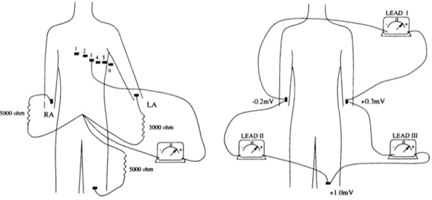
the patient runs on a treadmill. Figure 1.1 shows the location of the ECG recording leads on the body.

Figure 1.1: Standard leads used in ECG recording

QRS complex is actually three separate waves, the Q, R and S waves. All of them is caused by passage of the cardiac impulse through the ventricles. Figures 1.2 and 1.3 show typical heart beats recorded from standard channels.

Figure 1.3: Typical waveforms recorded

In the stress ECG records, the most important part of the beat is the ST segment (see Figure 1.2). Its depression or elevation reveals important medical information about the heart and is only observable during an exercise test. Figure 1.4 shows a typical heart beat with depressed ST segment. The reference DC level is the part before the P wave and after the T wave.

The problem in stress ECG is the high noise that contaminate it. There are two predominant types of noise: 1. Baseline wander noise (BW ) and electrode motion artifact. 2. Electromyogram-induced noise (EMC) [2]. BW is at a lower frequency, caused by respiration or motion of the patient or the leads. Frequency range of BW is usually below 0.5Hz and overlaps with that of the ST segment under stress. EMC noise, on the other hand, is at higher frequencies caused by increased muscle activity and by mechanical forces on

the electrodes. Its frequency range overlaps with that of ECG. Comparison of frequency spectra reveals the fact that direct filtering cannot be applied because it would distort ECG signal.

The stress ECG enhancing algorithms reported, compute a composite beat, an average beat in other words, and then make measurements on that beat. The following approaches can be found in the literature [3-8] :

M ea n C o m p o s ite : It is computed by averaging a set of noisy beats which are time aligned using a fiducial point, such as the peak of the R wave, in the heart beat. If the noise is uncorrelated with the signal, is stationary and has a Gaussian distribution, SNR is improved by \//V (N is the number of samples). However that is not the case, especially in stress ECG. If one of the beats has a sudden baseline shift or is an ectopic beat, a type of arrhythmia, the resulting composite will be distorted. So a preprocessing is needed.

M e d ia n C o m p o s ite : It is determined by computing the median of sample values across a set of beats, for each time instant. Time alignment is also done. This technique removes any outliners thus is capable of removing baseline shift or bursts of high frequency noise. It is computationally involved.

H y b r id C o m p o s ite : This approach combines the benefits of mean and median composite. A sequence of beats are grouped into three groups by one of the following strategies: 1. Random grouping partitions beats into three random groups. 2. Block grouping sequentially puts each one third into a group. 3. Sequential grouping puts sequential beats into different groups. Arithmetic mean of each group is calculated. Then, estimated baseline level is subtracted from each mean and a low-pass filter with a cut-off frequency of about 15Hz is applied. The output makes up the low frequency (LF) signal.

The difference between the filtered and original composites make up the high frequency (HF) signal. Thus HF and LF average beats for each group are obtained. The median of the HF composites is summed with the median of the LF composites. This approach is near optimal for high frequency noise, good for low frequency noise and is computationally efficient.

T rim m e d M ea n C o m p o s ite : It is computed by disregarding the bottom 20% and the top 20% of the sorted sample values for each time instant. Then the left are averaged. Thus it incorporates the feature of median filter by disregarding outliners and the feature of mean composite by taking averages, i.e. optimal when noise is Gaussian.

In crem en ta l C o m p o s ite : This approach is based on increasing or de­ creasing each sample value in the current (running) composite beat by a fixed amount. The direction of increment depends on the sample value of the next coming noisy beat with respect to the current composite. If it is higher, cur­ rent composite’s corresponding sample value is increased or vice versa. This approach provides a balance between immunity to noise and dynamic response of the composite.

F ilter B an k [9]: This approach is based on a filter bank (FB) containing a set of analysis filters that decompose the input signal into several sub-bands and a set of synthesis filters that combine them to get the complete signal. Signal processing is done in between according to the application. Since signals contain specific energy distributions in frequency domain, time and frequency dependent processing is beneficial. FB allows this processing. There are some unavoidable distortions due to non-ideal transfer characteristics of the filters and due to aliasing.

Our approach, different than the previous approaches, depend on orthogo- nalization of input channels. The algorithm used for orthogonalization is a Sin­ gular Value Decomposition (SVD) based online orthogonalization algorithm. It was first applied to separate maternal and fetal ECG by Vanderschoot, et al. [1]. Input ECG channels are orthogonalized and less number of orthogonal channels which carry all the ECG information are produced. They have no redundancy. The use of correlations between the input channels, increases the noise immunity of decomposed signals. Moreover, EMG and BW are repre­ sented in the output channels which are orthogonal to the ECG containing ones. This is a computationally efficient method and runs online. This ap­ proach deals with each beat one by one with the aim of recovering all rather than directly disregarding outliner sample values or averaging.

The existing commercial ST analysis software uses composite beats to make measurements. Performance evaluation is done in the same way, using our al­ gorithm as a preprocessing tool to enhance the ECG. Average beats of 20

I

second episodes are calculated and then analyzed. The enhancement we ob­ tained allows beat by beat analysis of the ECG, but for comparison purposes, the existing method is preferred. .-\s a result of noise elimination by orthog- onalization, more beats can be detected. This means more beats are used in the computation of composite beats. Even during complete loss of a derivation we can generate that derivation from other signals with limited error. This provides an uninterrupted exercise ECG test. These improve the quality of analysis. 23 exercise ECG records whose length range from 9:00 min. to 21:20 min. are analyzed. Each data set contains S independently recorded ECG derivations, namely DI, DII, VI, V2, V3, V4, Vo and V6. ECG is sampled at 500 samples/sec. Data is quantized with a 12 bit A /D converter with a dynamic range of 12 mV. The conclusions and the decision rules reported are empirical. They are concluded after exhaustive analysis of these data sets.

Chapter 2

THEORY

2.1

SVD And Its Basic Properties

The concept of orthogonality is widely used in signal processing. Orthogonal subspaces contain independent information, thus avoid redundancy. Golub and Van Loan [10] make the definition of orthogonality as follows;

A set o f vectors { x i ,. .., X p } in R ’'" is orthogonal if x j x j = 0 whenever i ^ j and orthonormal if x j x j = 6ij. If basis vectors of two subspaces are orthogonal to each other then they are called mutually orthogonal subspaces and contain maximally independent information. And a matrix Q is said to be orthogonal if Q ^Q = I.

The matrix 2-norm and Frobenius norms are invariant with respect to or­ thogonal transformations, i.e.

IIQAZIIf = IIAIIr IIQAZII, = ||A|h

(

2

1

(

2

2

provided Q ^Q = Z^Z = I.

Among various orthogonal transformations. Singular Value Decomposition

(SVD) is extremely useful concerning the information it provides about a given

m-by-n real matrix:

U = [UiU2...U ^ ] G V = [V1V2.. .V ,] G R '‘ "" (2.3) (2.4) such that U ^ A V = S = diag{ai,(T2·, ■ · ·, CTp) G p — rmn(rn,n) (2.5) where <y\ ^ cr-i > ■ ■ ■ > CTp > 0

Proof can be found in [10].

U ,V and S provide the following information about A at first [11];

k{A.) = k (7 k+\ — ^ k+2 — ■ · · — — 0 (2.6)

fl(A ) = sp a n (u i,. . . , UA:) (2.7)

Ä " ( A ) = sp an (u jt+ i,...,u ,n ) (2.8) 5 (A ) = s p a n (v i,. . . , va;) solution space of A (2.9)

N (X ) = sp a n (v A :+ i,...,v„) (2.10)

There is an important relationship between SVD and the eigenvalue de­ composition of the symmetric matrices A ^ A and A A ^. Since

x ^ A ^ A x = (A x )^ (A x ) = ]]Ax]] > 0 x ^ A A ^ x = (A ^ x )^ (A ^ x ) = ]]A^x]] > 0

(2.11)

(

2

12

both A ^ A and A A ^ are nonnegative definite, i.e. their eigenvalues are non­ negative and their eigenvectors can be chosen to be orthonormal. So

If A G R '"^ ",m > n 7

(A ^ 'A )V = (U E V ^ )^ (U E V '^ ')V = VE'^'S = V A (AA^)U = (U SV ^)(U SV^)^U = U S S ^ = U

A = E^S = diag{a\, cr.j... a^)

A 0

0 0

(2.14) (2.1.5) (2.16)

VV'e can conclude that the singular values of A are the square-roots of the first min(m,n) eigenvalues of A ^ A and A A ^ . The left and the right singular vectors of A are the eigenvectors of A A ^ and A ^ A respectively [11].

The definition of rank can be misleading in the presence of noise. Rank decision gains crucial importance especially in an online algorithm where you do not have the full data matrix. SVD is a powerful tool for rank determination, because it provides information on how near a given matrix is to a matrix of lower rank [lOj:

Lei the SVD o f A e be given. If k < r = rank{A ) and

Afc = X ] (TiU. vJ

1=1

then

II A- 1^1|2 l|A· A.1;||2

thus the definition

(2.17)

(2.18)

ra n k {A ,e) — mfn||A-B||2<i^<^^^^(B) (2.19)

becomes

Vc = ran k{A , e) ^ CTi > . . . > ar^ > e > > . . . > <Tp (

2

20

Finally we shall have a look at SVD related projections [10]:

Suppose

and U = [U ,U then V r V j = u . u ? ’ = J.j and V = [V,V,| ₍2.21)

projection onto null{A)'^

range(A^) (2.22)

projection onto null{A ) (2.23)

projection onto range(A ) (2.24)

projection onto range(A)^

null{A^) (2.25)

Equation 2.24 will be tlie basis of the online algorithm.

2.2

Basis Of The Online Algorithm

2.2.1

Mathematical Basis [1]

m = [mim

2

is received at each time instant. The data matrix which is constructed by collecting all these vectors, Mgxnj can be decomposed using SVD as

M = U E V ^ (2.27)

It should be noted that for a given M , the set of singular vectors, within a change of sign, and the singular values are unique provided that all singular values are distinct [11]. In case of equal singular values the singular vectors are not unique but the space spanned by them is.

A recursive property of each u,· is

u f M = _(2.28)

||M^x||/|lx|| < IIMV'II = <7. Vx e , x^Uj = 0 , j = 1 ,..., i' - 1

(2.29)

III words, u, represents a filter in space for which the samples of the output signal reach a maximal rms value, where u, is constrained to be orthogonal to U i,. . . , u,_i. Physically, ||M^u,|| represents the projected energy along u,. Remembering that U is orthogonal, we can use these filters to gather projected energy along orthogonal directions. Ui represents the highest energy containing direction, because it corresponds to the highest singular value, ctj.

This is closely related to the rank problem. In ECG signals, the directions with small energy content are attributed to noise. The dimension of the rest gives the rank. This is precisely the effective rank determination. Given that the rank is r, the error made by excluding those dimensions is bounded by ar^i (see Ec|uation 2.18).

If we can determine Ur (see Equation 2.21) then we can make use of the projection U rU j’ onto range of M .

The relation between the eigenvalue decomposition of a symmetric and positive definite matrix and SVD (see Equations 2.14 and 2.15) is used to determine U. The online algorithm approximates U incrementally (see Section

2.2.2). Knowing r, rank(M ), Ur is found from Equation 2.21.

2.2.2

Online Algorithm [1]

The strategy is to make an online eigenvalue decomposition of M M ^ . Knowing that the subspace spanned by U (left singular vectors of M ) is invariant, it can be concluded that the subspaces spanned by U and Q j (eigenvectors of M M ^ ) will be the same. Thus the problem becomes an eigenvalue decomposition problem of a nonnegative definite symmetric matrix.

M M ^ can be made diagonal by using a series of orthogonal transformations as in Equation 2.30. Each Q is a Givens Rotation matrix [10] and product of

them miike up Jacobi Rotation matrix [10]. This transformation makes M M ^ diagonal by making an off diagonal element zero at each step. In other words, it gcithers the information on off diagonal entries onto diagonal entries. This property is due to the fact that it is itself an orthogonal transformation.

o o ■f ^ ' y 9 (2.30)

where Qk is the Givens rotation matrix given by

Qa; = I 0 0 0 ..

...

which makes Cij and Cji zero. Due to uniqueness

p^-p

span{ Qfc) = 5pan(U )

k=l

However, since M is not known beforehand we approximate it by

(2.33)

Mi = [a‘ ‘ m (ii).. .am(ii_i) m(i.)]

11

where a serves as a memory element. At each time instant, t,, we apply one Givens Rotation to make the maximum off diagonal element in absolute value, zero. Thus as M ,M f approaches to diagonal form. Ili—i Q t approaches to U.

The algorithm is:

fo r =

I ,

0

Q, is the Givens Rotation matrix that makes the maximum off diagonal element of B, zero, rht is the reconstructed vector (see Section 2.2.3).

a has a great effect on the performance of the algorithm (see Section 2.3.2). Good compromise were obtained with a = 1 — 2“ ^^.

2.2.3

Effective Rank O f M

Effective rank of M is determined by tracing singular values and looking for a gap between two consecutive ones.

Physically r = rank(M) is the dimension of EGG information containing subspace. From now on this r dimensional subspace will be addressed as Signal

Space and its orthogonal complement as Noise Space.

Reconstruction ignoring noise space yields noise-free, information dense sig­ nals. Reconstruction is done as

ríi¿ = U¿_is, m. = U ,_ i(U f_ im .) S¿ = [ s i . . . S r O ... 0 ] ^ 1T S{ — [ s j . . . Sr>Sr+l · · · ■Sp] (2.42) (2.43)

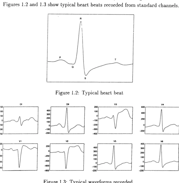
This is the projection onto range of M ( see equation 2.24). Figure 2.1 shows the input, decomposed and reconstructed data sets. There exist 8 channels

in the input data set, but most of the ECG information in these channels are collected in 2 orthogonal channels after decomposition. All of the 8 input channels are reconstructed from these 2 orthogonal channels. The error made is limited by the QRS energy in the third and fourth decomposed signal channels.

0 1 2 3 4 5 6 7 8 9 10

Time ( sec)

Figure 2.1: Input, decomposed and reconstructed signals (The input and reconstructed channels are

in the order of DI, DII, V I,..., V6 throughout the text)

2.3

Some Properties Of The Algorithm

2.3.1

C Matrix

C corresponds to Since this is an online algorithm, whole data matrix is not available. At each instant a single data vector is received. M is approximated using these vectors as in Equation 2.34. This corresponds to updating the C matrix as in Equation 2.38.

Diagonal entries of C correspond to squares of singular values. They are representatives of the energy contained along the particular direction pointed

by the corresponding u,·. Rank determination (which is found after exhaustive analysis to be either 2 or 3 in ECG signals) is done based on these singular values.

The changes in the relative values of the diagonal entries of C are indications of changes of information content along specific directions. Such a change is instrumental as a noise alarm (see Section 2.4.4).

The singular values corresponding to signal space and noise space also show the quality of the data recorded. If the singular values corresponding to the signal space are significantly higher than the rest, then data is noise-free. In some cases, the signal components are not strong enough with respect to the noise components, causing noise to be interpreted as signal (see Section 2.3.4).

The off-diagonal entries of C correspond to cross correlations between the output SVD channels. Making C diagonal means orthogonalizing the output channels. The algorithm makes the maximum off-diagonal element in absolute value, zero at each step. In other words, it weakens the relation between maximally correlated output channels.

Since the structure of C determines the evolution of U, we can direct U by manipulating C:

Enforcing a rotation limit when cq is to be made zero, prevents u,· and u_, from rotating at the same time more than the applied threshold. Physically it means preserving the dependency between these two output SVD channels. This seems to be undesirable, however, if these two vectors are in the same subspace then their interdependence causes no problem concerning the infor­ mation contained in that subspace. Such a threshold is applied for Ci2 when necessary (see Section 2.4.2).

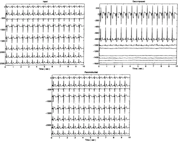
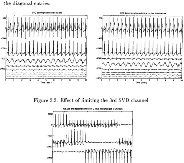
A rotation limit, when applied on c,* (for k = l , . .. ,p), keeps u, almost fixed. Thus we can preserve channels containing limited information to some extent. Figure 2.2 shows the effect of limiting Ca/t. After enforcing a limit on c^k the small ECG information present in the 3rd channel is kept in its place. The BW that contaminates the 3rd channel under limitless conditions, is shifted to the 4th channel.

If the structure of C is changed externally, the decomposed output signal set manipulates itself accordingly. This effect is extreme if the diagonal entries of C are reordered. After such a reordering the order of the output signals also change in the same way. Figure 2.3 shows the decomposed signal set when the

1st and 3rd diagonal entries of C are interchanged at 2nd sec. Within 10 sec. the 1st and 3rd SVD channels change place in accordance with the change in the diagonal entries.

SVD decomposition with no limit

500 r

IV

i

_i

V \a a A A A A A A / V \ A / V ^ /

1 2 3 4 5 8 7 8 9 10

Time ( sec)

SVD decomposition wrth limit on the 3m channel

> I

_\

E l

i U / l l i / U

1/ V W aH v V v v v v v v \ A A ^ V A 7 Vv

Time ( sec)

7 8 9 10

Figure 2.2: Effect of limiting the 3rd SVD channel

1 St and 3m dagonal entries of C were nierchanged at 2nd sec.

AiW A

r f fj' i

Figure 2.3: Decomposed signals when Cn and c.33 were interchanged

2.3.2

Memory Factor ,

a determines how far the algorithm remembers the past data. Good compro­

mise are obtained with a = 1 — 2“ ^^.

If it is too high then the algorithm loses its flexibility and cannot trace the changes in ECG signals. The u vectors remain almost fixed because C is not changed much with each coming data vector. If it is too low then, in the presence of noise, it cannot preserve the signal space even for a short time. It interprets noise as signal. Even QRS complexes may cause rotations of u ’s under noise-free conditions.

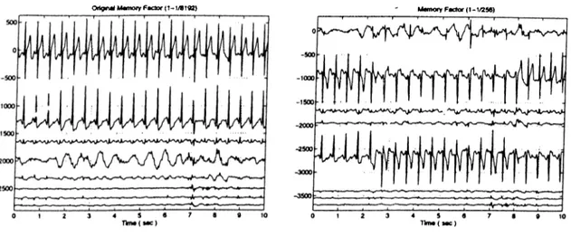
i^igure 2.4 shows the decomposed signals of the same input data set with different a values, 1 — 2··^^ and 1 — 2“ ® respectively. For small a values, the algorithm cannot preserve the ECG signals and they shift in between output channels.

O il^ n ^ Mamofy Factor (1 - 1/8192) Mamory Factor (1-1/256)

Figure 2.4: SVD with different a values

2.3.3

The Q M atrix

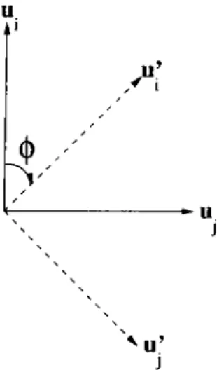
Product of all Qjt’s is called the Jacobi Rotations Matrix [10] (see Equation 2.30). It is the same as Givens Rotations. Q, as given in Section 2.2.2, performs a rotation o f the vectors and Uj in clockwise direction with an angle <f> on the plane defined by u, and Uj, as in Figure 2.5. In the algorithm, i and j are chosen to be the indices of the maximum off-diagonal entry o f C in absolute value.

<i> is chosen such that after the following transformation

Q ^ C Q = C (2.44)

C ’s maximum off diagonal element is made zero. Since

u.

u

^ u ’

Figure 2.5: Rotation of u ’s

this transformation is an orthogonal transformation. We do not lose any infor­ mation present in C

If 0 is limited, smaller rotations will occur. This will result in non-zero results for the chosen off-diagonal entry of C.

2.3.4

Importance O f D II

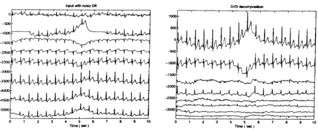
.Algorithm is very sensitive to noise in DII because it is the least redundant input channel due to its spatial position on the body (D ill is evaluated from DI and DII). Figure 2.6 shows the positions of D derivations on the body.

Dl

Input wtth noisy Oil SVO dscomposition -500 1000 500 -looop -1500 -2000 |/\4a4^v|/ij|a4^ ^^\AaJİ/\A/\XOî'\X^^^ -3000 -3500 -4000 -t500 5000

-i4'

F

Figure 2.7: Input and decomposed signals when DII is noisy

The leads on the body used to record EGG signals, record the potential differences occuring on the surface of the body due to the action potentials on heart. Heart can be thought as a dipole with some specific orientation. The currents on it flow in accordance with this orientation. DII is the only lead that is concerned with the currents’ projection on the direction from right arm to left leg (same as the position o f heart in the body). If D ill were recorded independently, this dependence on DII could be lowered because only then there would be an alternative input channel to DII. Figure 2.7 is an example of the performance of the algorithm in case of undesirable DII. The high noise in DII is completely observable in the most significant SVD output channel, the 1st channel.

Generally, if QRS is seen in the third SVD output channel, this comes from DII. Because of this if noise accumulation is detected at the third SVD channel during noise detection (see Section 2.4.4) (and if that channel is a QRS containing channel), DII is selected as noisy input channel at first. This choice is obviously a first estimate and may be erroneous. Such an error is preferred to missing noise because we can reconstruct the excluded input channel, though with limited error. Including D ili into the input data set as an independently recorded signal would reduce such errors by increasing redundancy.

2.4

The Method

The program is implemented in Borland C-f-+ under Windows 3.1.1. And it was run in 486 DX 4 IBM compatible PC. The flow chart o f the program is given in Figure 2.8. The explanations about the specific parts follow.

C O c •-1 a> to bo o O tr P 1 .D im e n s io n = 4 o r Fal se A la rm ( R o tat io n a n g lo th r e s h o ld a n d rotation an g le < 1 .2 5 thre sho ld a n d n o n o is e p o w e r in cr e a s e ) 2 .M u lt ip le S p ik e de te ct e d i: sa m p le in d e x i_ x ; p re v io u s s a m p le in d e x m e m o ry c o u n te r : s h o w s p o s it io n in t h e c y c li c m e m o ry o f 5 0 0 0 sam pl es 3 . (R o ta ti o n ang le > thr eshold a nd hig h n oi se p o w e r increa se Xor (R o ta ti o n an g le > 1 .2 5 th re sh ol d) o r (N o is e a cc u m u la ti on ) 4 . M o re t h a n 3 n o is e d e te cti o n a t th e same in st a n t

2.4.1

High Pass Filter

SVD is sensitive to DC components in input signals. DC is interpreted as a signal component and number of QRS containing output channels increases to represent the DC in the input. This leads to an increase in rank and inefficient compression of information. Figure 2.9 demonstrates the effect of non-zero DC in the input, on the output. The number of orthogonal signal channels is more than it should be when HPF is not applied. Note that the extra channel contains QRS complexes with almost the same morphology with the first SVD channel. This means that the 3rd channel exists only to represent DC.

SVD wrth HPFlng SVD without HPFing

Time ( sec) Time ( sec)

Figure 2.9: Effect of DC

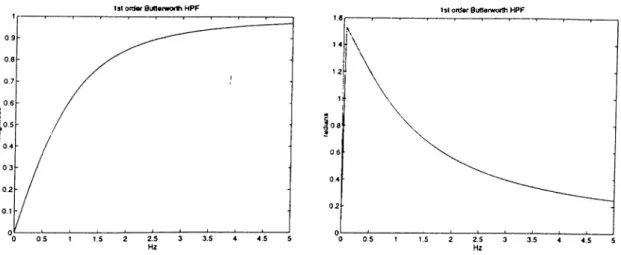
To avoid those redundant output channels, a first order Butterworth high pass filter with a cut-off frequency of 0.7 Hz, is applied to the input. Besides DC, very low frequency baseline variations are also eliminated. Since the filter is first order, it does not change the morphology of the signal significantly and is fast.

For faster operation, the coefficients were selected to be powers of 2. The transfer function of the filter used is

H(z) =

l - ( l - 2- ' ) z - '

1st ontor Suttarworih HPF 1st ordar Buttarworth HPF

Figure 2.10: High Pass Filter characteristics

2.4.2

Orthogonalization

The algorithm given in Equations 2..35 to 2.40 is implemented in this step. Only the reconstruction, Equation 2.41, is left to other steps.

Before creating Q ,, it finds the maximum off diagonal element. Since B,· is symmetric, a search algorithm may choose (i,j) or (j,i) equivalently. The difference will be in the sign of rotation angle , (f> , computed ( see Equation 2.32) because c „ ’s are in order of magnitude. We search in such a way that c„ is alw'ays greater than Cjj. Thus, sign of (p is only dependent on the sign of Cij chosen.

If rank is 3 , that is, if we need the third SVD output channel during reconstruction, we limit <f> when C3k{k = 1, . . . ,8) is chosen to be made zero.

This limits the rotation of U3. It is necessary because in any case the third SVD channel is a low energy containing one and is not immune to noise.

Besides, if energy in the first and second SVD channels are close to each other we limit c^ , that is simultaneous rotation of Ui and u-2 is prevented. This is done because when they are close to each other in the energy content, it is very likely that C12 will be the maximum off-diagonal element most of the time. That will cause Ui and U2 to rotate simultaneously. Their rotation does not make any difference considering the reconstruction process because signal components are still kept in the signal space. Such rotations, on the other hand, cause false noise alarms.

The bound applied to <p is 0.001° in absolute value. This value was found

empirically. It corresponds to 5° of rotation at maximum between two consec­ utive noise checks. This is the maximum rotation angle ob.served in most of the data under noise free conditions. Thus, our limiting causes the rotation to be more homogeneous rather than avoiding rotation completely.

.Angle limiting is not a preferred method because tracing the rotation di­ rection of u vectors performs best in the absence of such limits. It is also the most secure way of noisy input channel identification.

The program decides on limiting 4> or not. at the stage of Rank Decision (see Section 2.4.3). The relative energy content of the output SVD channels is checked by inspecting the diagonal entries of C, to decide on the limits to be applied. Weak signal channels are preserved by enforcing rotation limits on them. Strong ones are left free. The rotations in between strong signal channels are limited to avoid redundant rotations because they cause false noise alarms.

2.4.3

Rank Decision

First 30 seconds of the data is assumed to be noise free. Parameters are set according to the values at the 28th second.

Exhaustive analysis of ECG records showed that the rank of M is 2 and in few cases it is 3. This means information in ECG signals can be represented in 2 independent channels. So we are only concerned with C33 to decide on the rank.

The high amount of ECG information containing channels are named as signal channels. The decided effective rank is used to determine the number of signal channels. They are checked for their rotations during noise detection. The rest of the channels are named as noise channels. Their rotation is not important. Noise channels are checked against noise accumulation (see Section 2.4.4). If high noise energy accumulates in one of them, then that channel interferes with a signal channel.

In some cases, even though the effective rank of M is decided to be 2, the ECG information content of the 3rd channel cannot be disregarded. In such cases, although the highest energy containing 2 SVD channels are taken to be the signal channels, the 3rd channel is also included in the reconstruction. This

3rd channel is checked against noise accumulation, as if it is a noise channel. Whenever the 3rd SVD output channel is included in the reconstruction, csk

If the energy content of the 1st and 2nd SV'D output channels are close to each other, it is very likely that will be chosen as the ma.ximurn off diagonal element of C most of the time. This causes simultaneous rotations of Ui and U2· Such rotations do not cause loss of ECG because these 2 signals are in the same subspace, signal space, but they cause false noise alarms. In such data sets, rotation angle, <p, when C12 is chosen to be made zero, is bounded. This limit prevents Ui and U2 from rotating at the same time, avoiding false noise alarms. This limitation also causes an inefficient orthogonalization of these 2 channels. They remain somewhat correlated but this does not cause information loss (see Section 2.4.2).

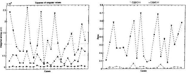
Generally noise accumulation check is done with respect to C22 as it is the weakest signal channel. In some cases, the 2nd SVD channel is so weak that, noise accumulation check with respect to that channel causes frec[uent noise alarms. Most of them turn out to be false alarms. Then, noise accumulation check has to be done with respect to Cu. The decision is given by checking C22. Figure 2.11 shows the highest 3 diagonal entries of the data sets analyzed at the time of rank decision, i.e. at the end of the training step.

{k = I,.... 8) is limited to preserve the low energy ECG signal on it.

Squares of singular values 'C 2 2 /C 1 1 İ-C33/C11

----1----1----1----1----1----r-\ 1 —1— 1— 1— r—1— r—1— I— 1— 1—1—1—1— 1—1— 1— 1— 08 — :---- 1— 1— ---1— 1— I— 1— 1— 1— T----1----1---- --- 1----1----1----1----1----1----1----1----1---» _0.7 1 ' 2 - ' ' ; ■ ; '! i 0 6 T * 1 / 1 ^ 1 ' k 1 0.5 / ' ! '1 1 1 / / 1 r / ■ 5 - \ ' ] ; • 1 . /» ; ' ■ a ( · / ‘ f ' 1 \ 1 \ ? ' f \ : \ ' V' 11- » k I-! \ ;...^ ^ V - ...i - 0 3 a , / 1 \ ; ; ' i ■ , V « ^ \ ¥ ; * f \ ^ ; ^-'*1 ; ■.<' 1 r ' * ' ' ' ’ 11 5 - \ M ' !_{)№- a} \1 . ¥ ' / _k-a \ a-ir -^"a u /n ^ / V ’ : H*-«-». «^a--a'“'ll·-a-a- «-*-HU -0 2 0.1 0 ; / V 1 A , S.'“* ' ' ‘1 1 ^ * ' * V* 'i __

Figure 2.11: Diagonal entries of C

Whenever a rotation angle limit is applied, or there is extraordinarily high energy content in an SVD channel, the angle thresholds, used in noise detection, has to be readjusted.

These checks need to be done independently. None of them implies another one. For example, deciding on a rank 2 condition does not imply that 2 SVD channels are enough to keep all the ECG information. There are cases like reconstructing from 3 SVD channels when the decided effective rank is 2. The

following decision rules are found empirically after intensive analysis of 23 exercise ECG data sets of length ranging from 9:00 min. to 21:20 min.

The default settings are: No limit on rotations is ¿ipplied, .SV'D and recon­ struction are done for 2 channel conditions, rotation angle threshold for the first SVD channel is 0.31 radians {thi) and for the second SVD channel it is 0.40 radians (tho), noise accumulation check is done with respect to the second .SVD channel.

The checks are done in the given order and necessary readjustments are done accordingly.

C22 > 0.3448 X Cii = > Limit C12 = > tht = 0.20 rad. ,th2 = 0.35 rad.

i.e. the 1st and 2nd SVD channels are so close to each other that rotations in between them are likely. They can cause false noise alarms. Even though this limitation avoids their being orthogonal to each other to some extent, this is not important because we keep the ECG signals in the signal space.

C33 > 0.04 X Cti reconstruction from 3 channels Limit C3k

i.e. the 3rd SVD channel should be used in reconstruction. The corre­ sponding basis vector must be kept fixed with some threshold to keep the information on it.

C33 > 0.25 X C22 = > rank(M) = 3 No rotation limiting

i.e. the 3rd SV'^D channel carries information comparable to the 2nd SVD channel’s. So it will be used in reconstruction. The noise effect on U3

can be detected from its rotation just like the 1st and 2nd SVD channels. The angle threshold used for the 3rd channel is th2.

C2 2 < 0-09 X 10* = > Do noise accumulation check wrt 1st SVD channel

i.e the 2nd SVD channel does not contain much ECG energy, hence noise energy should be compared with the energy of the 1st SVD channel to detect noise accumulation.

rank(M ) = 2 C22 > 7.00 x 10* =i> thi = 0.10 rad. , th^ = 0.15 rad. i.e. ECG energy in the 2nd channel is so high that smaller rotations can cause signal vectors to take on noise. The thresholds are lowered.

These thresholds, used in decisions, depend on a. Since clinical data were used to determine the above rules, they reflect the real values that one can come across. The readjustments made, improve the performance of the program, especially its noise detection capability. The ST analysis results reported in Section -3.2 were obtained by applying these rules.

In general, it is concluded that the ECG signals can be represented in 2

orthogonal channels with enough accuracy for Exercise ECG Test.

2.4.4

Noise Detection

In order of importance, rotation of the basis vectors of the signal space, noise accumulation in the most significant noise channel (in case of reconstruction from 3 channels when ra n k (M )=2, the third signal channel is also checked for noise accumulation) and total noise energy increase are checked at every 10

seconds.

First, rotation of the basis vectors is checked. If anyone of them has rotated more than the corresponding threshold, this indicates that the rotated basis vector began to take on noise. Signal space’s basis vectors are highly stable and do not rotate much in the absence of noise. Thresholds applied are:

If Ci2 is limited , the threshold for Ui is 0.20 radians, and 0.35 radians for U2

and U3. If C12 is not limited then these limits are 0.31 radians and 0.40 radians respectively. If C22 < 7-00 x 10® ( see section 2.4.3 ) then they are 0.10 radians and 0.15 radians respectively. Threshold for Ui is less then the others because although it is more stable, its smaller rotation causes more loss of information. So we have to be more careful in watching Ui. Note that when rotations are limited, thresholds are lower not to miss noise.

When a rotation more than the threshold occurs, total noise energy increase is checked. If it has not increased at least 1.5 folds within the last 10 seconds then alarm is considered to be false. The eussumption here is that if noise arrives, it cannot be represented completely in the signal space. Energy of the noise channels must also increase.

Against the possibility of noise being observable completely in signal space, we check the rotation angles against 1.25 x threshold. If such a high rotation has occured then it is decided on the existence of noise directly, without checking the total noise energy increase.

If vector rotation is not detected then noise accumulation is checked. Low frequency, high amplitude noise do not rotate signal space vectors significantly but accumulate in a noise channel for some time. When the corresponding diagonal entry of C gets high enough, noise interferes with the signal space. At that instant, we cannot identify the noisy input channel. So all we can do is to detect such an accumulation on the most significant noise channel when it starts and identify noisy input channel from the corresponding u.

Figure 2.12 shows an example of noise accumulation. The BVV' in the 3rd SVD channel interferes with the signal in the 2nd SV'D channel after 30 seconds. The energy of the 2nd channel and BVV' are close to each other and as a result the algorithm cannot keep them separated for more than 15 sec. This is same as interchanging the 2nd and the 3rd diagonal entries (see Figure 2.3).

BW accumulated on 3rd SVO channel

If ^kk ^ 0.24Cfi

Ckk — ^^^^(^(r+l)(r+l)? · · · 1 ^8s) ) ^ Tflii At(M )

^ \ C22 < 0.09 X 10* 2 C22 > 0.09 X 10*

t =

then it is decided that noise has accumulated on SVD channel.

Accumulation check is done with respect to cn or C22 rather than Crr because even when r=3 , energy in the third channel may be close to noise energy. This check is not indicative in that case. Noise may not be observable in the third SVD channel.

1 2 1 15 C(1.1) C(3.3) 10 IS 20 25 30 35 40 45 Time (sec) 10 15 20 25 30 Time (SBC) C(4.4) 40 45 50 15 .0 5 ^ : ... 0 ---1---1---1---1---1---1---1_______1_______1_______ 1__ 20 25 X Time (sec) 0 5 10 15 20 25 X 35 40 45 50 Time (sec)

Figure 2.13: Energy content of SVD channels

A multiple spike (spike in most of the input channels, usually in all) check is also applied. During the experiments , it was observed that if a spike (short duration, even instantaneous, high amplitude noise) arrives, total noise energy graphic exhibits a jump and then falls to its old value rapidly. This fast fall is detected. If slope is over a threshold of 64mV^/sec then it is considered as a multiple spike, no dimension reduction is applied, old U and C are recovered to avoid the rotation effect of it.

Figure 2.13 shows the graphics of diagonal entries of C of EMG contami­ nated exercise ECG data set. The time when the noise starts is the time when the jum p in the graphics corresponding to noise channels, occurs.

2.4,5

Noisy Input Channel Identification

Noise is detected in two ways, either signal vectors rotate more than a thresh­ old or noise accumulates on a noise vector or on U3 as a special case (u.3 is considered as a noise or signal vector depending on the energy it collects).

The former is an abrupt change. If the cause of noise detection is a rotation then we look for the direction of rotation. The vector rotates to take on noise. The component of the vector which experienced maximum increase in absolute value corresponds to the noisy input channel.

The latter is a slowly evolving change. At the time of accumulation detec­ tion, it has already directed towards the noise. That is, the vector’s maximum component in absolute value shows the noisy input channel. The direction of rotation within the last 10 seconds can be misleading in such a situation be­ cause the vector usually tries to turn towards the clean input channels during accumulation. If it succeeds then no accumulation occurs.

2.4.6

Dimension Reduction

Since

s = U^m (2.47)

the rows of U can be associated with input channels whereas the columns with the output SVD channels.

Decreasing dimension by one means deleting the selected input channel and an output channel. The input channel is selected by noisy channel identification (see Section 2.4.5). The output channel is always selected to be the weakest SVD channel, i.e. the last noise channel. The corresponding row and column are deleted from U. The new U is re-orthogonalized by Grarnschmidt Method [12] to maintain orthogonality. This process starts with the leftmost column of U, keeping it unchanged (the highest energy containing signal vector), proceeds towards the weakest noise vector.

The rows and columns of C correspond to the output SVD channels. The last row and column of C are also deleted.

the rows and columns shown by * in the following are deleted.

2.4.7

Noise-OfF Check And Dimension Increase

At every 10 seconds, two peaks are found at each input channel towards past. If ECG is noise-free then these two peaks are R peaks of QRS complexes (For input channels V I, V2 ,V3 minimums rather than maximums are found due to their morphologies ( See Figure 1.3 )). Duration of a QRS is around 0.2 seconds which corresponds to 100 samples. Total error between time intervals of 0.2 sec. around these two peaks is calculated. Then a threshold is applied to its ratio with the QRS energy of that channel. The applied threshold is determined for each channel during training. They are bounded by a minimum of 0.2 and a maximum of 0.8. Too high thresholds would result in false noise-o^ decisions. Too low ones would miss noise-off. Bounds are put to avoid these.

Whenever noise-off is found, the most recent 8 dimensional U and C are reduced in dimension excluding the still noisy input channels. Reconstruction coefficients are also updated according to the new U.

2.4.8

Reconstruction

Since U is an orthogonal matrix

U - ‘ - , m = U (U 'm ) - Us _(2.48)

Equation 2.48 reconstructs the input channels from SVD outputs identi­ cally.

To e.Kclude the orthogonal noise components during this reconstruction , s is used instead of s, i.e. we e.xclude noise channels from the decomposed vector. In noise free conditions , these channels are almost zero. Thus we guarantee that we do not exclude ECG information.

s = 5i .S2 s, 0 . . . O j r = 2,3 (2.49)

m = Us (2.50)

Reconstruction from 2 or 3 channels depends on the rank of the data pro­ cessed. -Although, usually two channels are used, in some cases 3 channel reconstruction becomes a must. In 2 channel reconstruction, we sacrifice some QRS energy that is left in the third channel, to exclude noise. The examples in Figure 2.14 are noise-free cases so the sacrificed QRS energy is fully observable. The differences mainly occur in the amplitudes of the peaks. Avoiding noisy output was preferred to capturing all QRS energy in noisy parts. The lost QRS energy is not much and not significant for ST analysis in E.xercise ECG Test. The difference mainly occurs at the amplitude of the R-wave. Table 2.1

gives the energies of the original QRS complexes and reconstructed ones under noise-free conditions. They are computed by

noo _{rrik is the sample value}

Channel QRS SS 2 ch. rec. SS S ch. rec. SS

DI 288 278 300 DII 1803 1703 1812 VI 1263 1226 1290 V2 4029 3911 4044 V3 14422 14575 14440 V4 3654 3355 3546 V5 2049 1885 2010 V6 3331 3276 3275

Table 2.1: Comparison of 2 and 3 channel reconstructed QRS energies SS : Sum of Squares

Figure 2.15 shows a comparison of the reconstructed ECG signals by using SVD coefficients and LMS-Newton [13] coefficients, from the most significant

Ol originaJ, 2 0 and 3 0 reconstructed Oil original. 2 0 and 3 0 reconstructed

- : input , : 2D , - - : 3D

Figure 2.14: 2D versus 3D Reconstruction 31

Wo ~ [0 0]^ for i Pi tt’.+i Q = 0.005 = 0 to N T = Wi Si = W i+ 2a(di - pi)Rs,-i.i

where p is the predicted signal, w is the vector of coefficients, s is the input signal vector (it is SVD signal channels in our case), d is the desired signal (the original form of the reconstructed signal), R is the estimated autocorrelation matrix of input signals.

Both reconstructions are very close to each other. They differ from the origirial signal at P and T waves, and at the amplitude of R wave. Such errors can be eliminated by including the .3rd SVD channel in the reconstruction. Since the third channel is not immune to noise as much as the others and since it does not carry significant information about the ST segment much, it is preferred to exclude it. The ST segment of the beat carries the most important information for Exercise ECG Test. Both of the reconstructed beats are almost the same and SVD fits better in V' derivations.

The errors made in reconstruction per QRS complex are computed by SS of error SS of original QRS SS of error SS of original QRS nil nik v^lOO ( \2 VlOO 2 ^k=\^k

Sample values of the reconstructed beat Sample values of the original beat

The errors in percentage are given in Table 2.2.

In the case of reconstruction of totally lost input channels the most recently used coefficients for that channel before excluding it, are used (see Section

3.1.4). The assumption here is that they do not vary much. This is reasonable since the only high variations are observed in the presence of noise. Whenever dimension is increased, reconstruction coefficients are updated.

Dl; Input, LM S-New ton and 2 0 SVO Reconstructions

Οβ: Input. LMS-Newrton and 2D SVD Reconstructions

V I; Input. LMS-Newion and 2D SVD Recorwlructiorw V2: Input. LMS-Newton arxi 2D SVD Reconstmctions

ѴЭ; Input. LMS-Newton and 2 0 SVO Reconstructions

VS; Input, LMS-Newton artd 2D SVD Reconstnictions

V4 Input, LMS-Newton and 2D SVD Reconstnictions

LMS-Newton Figure 2.15: SVD vs LMS-Newton reconstruction

Channel di DII VI V2 V3 V4 V5 V6 Error In S V D Recon. 4.33 % 2.68

%

Error In LM S-Newton Recon.

r.62 %

%

Table 2.2: Comparison of 2D and LMS-Newton reconstruction errors

2.5

Data Compression

This method improves the compression ratio of EiCG signals by eliminating noise.

Compression of information is a direct consequence of eliminating redun­ dancy in ECG signals by orthogonalization. After SVD, all the information can be represented in at most 3 independent channels. This means a compression of at least 3 to 8 without considering reconstruction of standard derivations. Reconstruction is assumed to be a redundant process because if arrhythmia analysis was done using these orthogonal signals, then data compression would be achieved by keeping only the orthogonalized signal set. Such a work was done by Çağlar [16].

Chapter 3

EXPERIM ENTS

3.1

Performance On Typical Noise Types

The capability of the algorithm is tested on various noise and artifact con­ taminated EGG records. Appendix A hcis examples from these data. Both EMG (Electromyogram) and BVV (Baseline Wander) are often observed on DI, which is a channel with low amplitude EGG signal. If such noise , especially BVV (low frequency, high amplitude noise), were on DII, a performance degra­ dation is unavoidable due to the special spatial position of DII on the body. Such noise generally interferes with the signal channels at the output of SVD. The algorithm is capable of filtering EMG noise and BW, which are the two basic noise sources in EGG signals. This filtering performance can be reached in even noisy DII cases by taking some precautions like recording D ill inde­ pendently (see Section 2.3.4). We will also demonstrate the reconstruction of a completely lost input channel from the information in other channels with limited error. Gorrelations between input channels are instrumental tools in these situations. The reconstruction in such a case uses constant coefficients, so it is not adaptive , however this is the best that can be done in the absence o f desired (lost in this case ) signal (LMS algorithms require the desired signal which is the totally lost one in this case).

3.1.1

E M G Noise

EMG noise is a high frequency noise caused by increased muscle activity par­ ticularly around the electrodes. Its frequency spectrum is wider than that of

ECG’s and overlaps with it. So direct frequency filtering to eliminate EMG distorts EGG signals. Filtering based on moving window averaging does not perform good because biological signals are not stationary. Averaging assumes the noise to be white but this is not always true. It can also distort EGG. These approaches does not make use of the correlations between input channels. Our approach uses the information in other ECG channels to compute the EGG in a noisy channel. Figure 3.1 shows a set of EGG signals with EMG contamination in DI. The decomposed and reconstructed signals are also shown. The EMG in DI is almost completely observable in the noise channels of the decomposed signal set. Reconstruction provides noise-free DI, as shown in detail. The small amount of EMG in DII and VI is also filtered out. The clean input channels remain unaffected.

Input ECG iignaJs Rdconstactad ECG s is a ls

-500 -1 0 0 0 -1500 -2000 -2500 -3 0 0 0 -2500 -3000 -3500 ^1000 0 t|AA|A^d|A>'|A^i|A^\|A'Aj^^ |V|Aq|V|V^ Aa /Ia. a^· a-*|a-'|aa|aa|^ a^^|aa/u Aa|aa^^V/v. Aaa 0 1 2 3 4 5 6 7 8 9 10 Tim e ( sec ) 0 1 2 3 4 5 6 7 8 9 10 Tim e ( sec )

Figure 3.1: ECG with EMG

3.1.2

Baseline Wander (B W )

B W is a low frequency noise caused by respiration and motion of the patient or leads. Its frequency components are usually below 0.5 Hz but during an