Piecewise-Linear Pathways to the Optimal
Solution Set in Linear Programming
1M. C. PlNAR2 Communicated by P. Tseng
Abstract. This paper takes a fresh look at the application of quadratic penalty functions to linear programming. Recently, Madsen et al. (Ref. 1) described a continuation algorithm for linear programming based on smoothing a dual l\ -formulation of a linear program with unit bounds. The present paper is prompted by the observation that this is equivalent to applying a quadratic penalty function to the dual of a linear program in standard canonical form, in the sense that both approaches generate continuous, piecewise-linear paths leading to the optimal solution set. These paths lead to new characterizations of optimal solutions in linear programming. An important product of this analysis is a finite penalty algorithm for linear programming closely related to the least-norm algo-rithm of Mangasarian (Ref. 2) and to the continuation algoalgo-rithm of Madsen et al. (Ref. 1). The algorithm is implemented, and promising numerical results are given.
Key Words. Quadratic penalty functions, linear programming, piece-wise-linear path-following algorithms, characterization of optimal solutions, finiteness.
1. Introduction
In a recent paper (Ref. 1) Madsen et al. gave a new finite algorithm to solve the problem
1This research was supported by Grant No. 11-0505 from the Danish Natural Science Research Council SNF. The author is indebted to K. Madsen, H. B. Nielsen, and V. A. Barker for their support. The careful work of two anonymous referees is also gratefully acknowledged. 2Assistant Professor, Department of Industrial Engineering, Bilkent University, Bilkent,
Ankara, Turkey.
619
where E is n x m , d e Rm, and feRm. The case where f=0 is precisely the linear l1-estimation problem (Ref. 3). A smooth approximation of (AL1)
was considered by Madsen et al. (Ref. 1):
The function p is known as the Huber function in robust regression; see Ref. 4. A finite Newton type algorithm was used by Madsen and Nielsen (Ref. 5) to solve (SAL1). Later, Madsen et al. (Ref. 1) showed that the set of minimizers of GY define continuous, piecewise-linear paths as a function of 7 leading to the optimal solution set of (AL1). They established that solutions to (AL1) and its dual (which is a linear program with unit upper and lower bounds) can be found for a sufficiently small positive value of the parameter j. By exploiting this property, a finite continuation algorithm to solve linear programs was given in the same reference with encouraging initial numerical results. Now, the present paper is prompted by the observa-tion that the ideas summarized in the above paragraphs can be used to solve the linear programming problem using quadratic penalty functions.
Consider the primal linear programming problem
where xeRn, A is an m x n matrix, beRm, ceRn. The dual problem to (P) is given by
where y e Rm. We define the dual penalty functional
and W is a diagonal m x m matrix with entries:
In this paper, we study the unconstrained problem
for decreasing positive values of t.
All the results and the algorithm of the present paper are obtained by combining the continuation viewpoint (Ref. 1) and a well-known duality and perturbation result in linear programming (Refs. 2, 6-10) to study the quadratic penalty problem (CD). This result states that, for t sufficiently small, a dual optimal point to the penalty problem (CD) is a solution of (P) with the least 2-norm. Using this result, we establish the piecewise linear behavior of the solution set of (CD) as t is decreased, and give novel charac-terizations of the solution set of (D). The main contribution of the paper is the design of a finite algorithm as a modification of the least-norm algorithm of Mangasarian (Ref. 2) using the ideas of Madsen et al. (Ref. 1). However, the algorithm of the present paper differs from the continuation algorithm of Ref. 1 in the strategy for reducing the parameter t and the stopping criteria. The algorithm of Mangasarian (Ref. 2) computes a least-norm solu-tion of linear programs based on the above perturbasolu-tion result and using a SOR (successive overrelaxation) algorithm. Our algorithm differs from this algorithm in two important aspects: (i) we use a modified Newton algorithm to compute a point on the paths; (ii) we use a new, effective reduction strategy for t that exploits the piecewise-linear nature of solution paths and yields primal-dual solutions in a finite calculation.
We give computational results of our algorithm using a small subset of the Netlib test set. The results indicate that the new dual penalty algorithm exhibits a performance comparable to the algorithm of Ref. 1 and to the dense linear programming system LSSOL from Stanford University Systems Optimization Laboratory (Ref. 11) on the test set. For more details on penalty and active set methods for linear programming, see Refs. 6, 12-16. While the present paper was under review, we have developed an appli-cation of the quadratic penalty functions to linear programs with mixed inequality and equality constraints. This is both theoretically and computa-tionally a nontrivial extension of the present paper and is described in detail in Pinar (Ref. 17). This also relates our research to early work by Chebotarev in the Russian literature (Ref. 14).
2. Pathways to Optimal Solutions
Let yt denote a solution to (CD) for some t > 0. It is well known (see,
e.g., Ref. 18) that every limit point of the sequence {yt} solves (D). Now,
define a binary vector seRn such that
Hence,
In the sequel, we drop the argument y when the meaning is clear from context. We denote by Y the set of optimal solutions to (D). We assume throughout the paper that A has rank m.
2.1. Structure of the Solution Set of (CD). In this section, we briefly
examine the properties and structure of the set of minimizers of H. The results of this section follow immediately using some results of Refs. 8 and 9.
It is evident that H is composed of a finite number of quadratic functions. In each domain DeRm where s(y) is constant, H is equal to a
specific quadratic function as seen from its definition. These domains are separated by the following union of hyperplanes:
A binary vector s is feasible at y if,
If s is a feasible binary vector, H is given by a specific quadratic function on the subset
We also call gs a Q-subset of Rm. The gradient of the function H is given
by
where W is the diagonal matrix obtained from a feasible binary vector s at
y. For yeRm\B, the Hessian of H exists and is given by
It is well known (see for instance Refs. 2, 6-10) that the dual of the quadratic penalty problem (CD) is given as
Let xt denote the unique optimal solution to the above perturbed
program, and let z+ denote a vector whose ith component is max{zi, 0}. It
is shown in Lemma 6 of Ref. 9 that
for any zteUt. That is, the right-hand side is constant regardless of the
choice of minimizer zt. Hence, we have the following characterizations of
the solution set of (CD) analogously to the solution set of (SAL1).
Lemma 2.1. s(yt) is constant for yteUt. Furthermore, rt (yt) is constant
for yeUt if st= 1.
Following the lemma, we let
as the sign vector corresponding to the solution set. Now, we can use Lemma 2.1 and the linearity of the problem to characterize the solution set Ut.
Corollary 2.1. Ut is a convex set which is contained in a Q-subset As,
where s=s(Ut).
Corollary 2.2. Let yt e Ut and s=s( Ut). Let Ns be the orthogonal
com-plement of Vs=span {aT\ si = 1}. Then,
2.2. Characterization of Optimal Solutions through Dual Paths. In
this section, we analyze the behavior of the solution set Ut as t approaches
zero. The main result of this section is given in Theorem 2.2.
Assume that yteUt and s=s(Ut), with W = d i a g ( s1, . . . , sn) . Then, yt
It follows from (13) that the following linear system is consistent:
Now, let x, denote the unique optimal solution to (PB). Then, we have from Li and Swetits (Ref. 9) that
for any yteUt. From Theorem 2.1 of Mangasarian (Ref. 2), we have that, for small enough t, for te(0, t0] say, xt is constant: it is the least 2-norm solution of (P). This implies that
for 0 < < S < t . Let
Then, one can rewrite the above as
Combining (15) with (17), we have
Multiplying both sides by A, and since Axt = b, we get
Hence, using Corollary 2.2, we have the following theorem.
Theorem 2.1. There exists t0>0 such that s = s(Ut) is constant for
0<t<t0. Furthermore, let d be a solution to (14) such that s ( yt + Sd) = s
for 0<8<t<t0. Then,
In general, it follows from the linearity of the problem that the set of minimizers Ut has a piecewise-linear structure. Combining this with Corollary 2.2, we have the following corollary.
Corollary 2.3. Let yteUt and let s = s(Ut). Let d solve (14). If
s(yt + ed)=s for e>0, then s(yt+ 8d)=s and
Since the number of distinct binary vectors is finite, we also have the following corollary.
Corollary 2.4. s( Ut) is a piecewise constant function of t > 0.
Combining the study of the piecewise-linear paths generated by the minimizers of H with Theorem 2.1 of Mangasarian (Ref. 2), Theorem 2.2 below gives a new characterization of the optimal solution set Y of (D).
Theorem 2.2. Let 0<t<t0, where t0 is given in Theorem 2.1, and let
s=s(Ut). Let yteUt, and let d solve (14). Then, U0 = Y, where
with
Proof. First, xt= - W r ( yt) / t is an optimal solution to (P) with least
norm by Theorem 2.1 of Ref. 2. Let ye Y. By the complementary slackness theorem, Wr(y) = 0. Now, let yteUt. Then using (13), we have
Hence, there exists a solution d to (14) such that y = yt + td. Since any solution d to (14) can be expressed as d=d+n, where n e N ( A W AT) ,
for any solution d to (14). Now, assume y0e U0. Then, there exists a solution
d0 to (14) such that y0=yt + td0. Therefore, we have
Now, y0 is complementary to x, and is feasible in (D) by definition of U0 and (21). Therefore, y0 is an optimal solution to (D). Since this holds for any y0eU0, U0< Y.
If Y is a singleton, the proof is complete. Therefore, assume otherwise. Let ye Y. Using (20) again, it follows that ( y - yt) / t solves (14) for any yt€Ut. Therefore, we have shown that y e yt + t d + Ns. Now, by virtue of
feasibility, yEDs for any ye Y. Hence, ye U0. D
3. Dual Penalty Algorithm
We now construct a penalty algorithm for linear programming similar to the finite continuation algorithm of Madsen et al. (Ref. 1) and to the least-norm algorithm of Mangasarian (Ref. 2). This algorithm is different from the continuation algorithm in two important aspects: (i) the choice of the reduction strategy for t; (ii) the stopping criteria. These differences make the algorithm a finite variant of the algorithm of Mangasarian. The algo-rithm of Mangasarian consists of solving the dual to (PB) using a SOR iterative scheme to compute a least-norm solution to (P). Our algorithm computes both a least-norm solution to (P) and an optimal solution to (D) in a finite calculation using the piecewise linear dependence of unconstrained minimizers on t. In contrast to the algorithm of Mangasarian, we use a finite Newton-type method to solve (CD), which is more accurate than the SOR method. On the other hand, the algorithm of Mangasarian is very simple, since it does not involve any matrix factorizations.
The algorithm is initiated by choosing values t0 and y0. A minimizer y0, of H using t0 is found. The general step k+ 1 for k>0 is given below.
Step k +1. Let yk denote a minimizer of H for tk. Choose tk + 1 and a starting point for subsequent iterations based on yk, and compute a
mini-mizer yk+1 of H.
The algorithm stops when the duality gap is zero (within roundoff) and both primal and dual feasibility are observed. Otherwise, t is decreased according to some criteria; see Section 3.2. To complete the description, we need an algorithm to compute a minimizer of H. Such an algorithm is adapted from the Newton algorithm of Madsen and Nielsen (Ref. 5) for robust linear regression using Huber functions; see Section 3.1.
Now, we define an extended binary vector j such that
We denote by W the diagonal matrix derived from s. We also define the following active set of indices:
This extended definition of binary vector is used in the detailed description of the algorithm and in proving its finite convergence.
3.1. Computing an Unconstrained Minimizer. Let y be the current iter-ate with W the diagonal matrix derived from s(y). A search direction h is computed by solving the Newton system
For ease of notation, let
Furthermore, let N(C) denote the null space of C. If C has full rank, then
h is the solution to (24). Otherwise, if the system of equations (24) is
consist-ent, a minimum-norm solution is computed. If the system is inconsistconsist-ent, the projection of g on N(C) is computed. These choices are motivated and justified in Madsen and Nielsen (Ref. 5). The next iterate is found through a line search aiming for a zero of the directional derivative. This procedure is computationally cheap as a result of the piecewise-linear nature of H'. It can be shown that the iteration is finite; i.e., after a finite number of itera-tions, we have that y + h is a minimizer of H; see Ref. 5 for details.
3.2. Reducing the Penalty Parameter. Let y, be a minimizer of H(y, t) for some t>0 and s=s(yt). Consider the system
Let d be a solution to (25). We distinguish between two cases.
Case 1. The duality gap cTx + bT(yt + td) is zero, but yt + td is infeas-ible in (D); i.e., there exists j such that rj( yt + t d ) < 0 . In this case, we reduce t as follows. Let o = {ak, k= 1, 2 , . . . , q} be the set of positive kink points where the components of r ( yt + td) change sign, i.e., the set
where
If o is nonempty, we choose a* = mink ak and we let
Notice that
where either B<0.9 or b = 1-a*, with 0 < a * < 1 , so that tnext<t. In both
cases, ytnext is used as the starting point of the modified Newton algorithm of Section 3.1 with the reduced value of t.
Case 2. The duality gap is not zero. In this case, we reduce t as follows. Let c((1 — €)t) denote the number of changes in the active set from I(yt) to I ( yt + etd). We use bisection to find a value e of e such that c((1 - e)t) x
1/2c(t), and use
For robustness, we search only in the interval [0.1t, t) so that tnext<0.9t.
3.3. Finite Convergence. Let S( Ut) denote the set of all distinct binary
vectors corresponding to the elements of Ut. That is, for any yteUt,
s ( yt) e S ( Ut) .
The following results are obtained as consequences of the linearity of the problem, Lemma 2.1, and the finiteness of the extended binary vectors. Lemma 3.1. If S(Ut 1) = S ( Ut 2) , where 0 < t2< t1, then S(Ut) =
S(Ut1) = S(Ut 2)for t2< t < t1.
Theorem 3.1. There exists t such that S(Ut) is constant for te(0, t),
where 0 < t < t0.
The following theorem is crucial for the finite convergence analysis. Since the proof is lengthy, we refer the reader to the more general analysis of Ref. 17.
Theorem 3.2. Let te(0, t) and yteUt, with s = s(yt) and x* =
-(1/t)Wr(yt). Then,
Lemma 3.2. Assume te(0, t). Let yeUt, with s = s(y). Let d solve (25), and let ynext be generated by one iteration of the penalty algorithm. Then, either
and the algorithm stops, or
where a* is as defined in Case 1 of the reduction procedure, and I(Ynext) is an extension of I ( y ) .
Proof. Let
Clearly,
from Theorem 3.2. Hence, we are in Case 1 of the reduction procedure of Section 3.2. If r(y + t d ) > 0 , then ynext=y + td is a solution to (D) by Theorem 3.2, and the algorithm stops. Otherwise, Theorem 3.2 implies that
I ( y ) < I ( y + td). Hence, using the definition of a*, we have
Since there exists jE{1,. . . , n}\I(y) such that rj(y + a*td) = 0,I(y + a*td) is an extension of I ( y ) . Furthermore, y + a* tdeEs. Therefore, using the continuity of the gradient H', (10), and the definition of d, have
Thus, Ynext minimizes H(y, (1 -a*)t).
Let y e Ut for some t>0. Unless the stopping criteria are met and the algorithm stops with a primal-dual optimal pair, t is reduced by a nonzero factor (tnext = Bt) as discussed in Section 3.2. Hence, {tk} is a strictly decreas-ing sequence convergdecreas-ing to 0. Since the modified Newton iteration of Section 3.1 is a finite process, t reaches the range (0,t). where t is as defined in Theorem 3.1, in a finite number of iterations unless the algorithm stops. Now, assume that te(0, t). From Lemma 3.2, either the algorithm terminates or the active set I is expanded. Repeating this argument, in a finite number of iterations the matrix AWAT will finally have rank m, since A has rank
m. When AWAT has full rank, the solution d to the system (25) is unique, and ynext = y + td solves (D) by Theorem 3.2. Therefore, we have proved the following theorem.
Theorem 3.3. The dual penalty algorithm defined in Section 3 termin-ates in a finite number of iterations with a primal-dual optimal pair.
4. Implementation and Numerical Results
In this section, we report our numerical experience with a Fortran 77 implementation of the dual algorithm, which does not exploit sparsity. The purpose of the experiments is to test the viability of the algorithm in solving problems of practical interest, and to compare it with the code LPASL1 of Madsen et al. with the package LSSOL from Stanford Systems Optimization Library. LSSOL is a Fortran 77 package for constrained linear least-square problems, linear programming, and convex quadratic programming; see Ref. 11. It does not exploit sparsity. Hence, it provides a fair comparison to our numerical results. We refer to the implementation of the penalty algorithm as LPPEN.
4.1. Numerical Linear Algebra. The major effort in the Newton algo-rithm of Section 3.1 is spent in solving the systems (24). We use the AAFAC package of Nielsen (Ref. 18) to perform this. The solution is obtained via an LDLT factorization of the matrix Ck = AWAT. Let us recall that Wu= 1 for the columns of A corresponding to indices in the active set / as defined in (23). Based on this observation, D and L are computed directly from the active columns of A, i.e., without squaring the condition number as would be the case if Ck was first computed. It is essential for the efficiency of the penalty algorithm to observe that, normally, only a few entries of the diagonal matrix W change between two consecutive iterations. This implies that the factorization of Ck can be obtained by relatively few updates and downdates of the LDLT factorization of Ck - 1. Therefore, the computational cost of a typical iteration step is O(m2). Occasionally, a refactorization is performed. Details are given in Ref. 18.
For the solution of (25), the matrix A WAT is identical to the last Ck used in the Newton iteration. Thus, the LDLT factorization is available. In order to enhance accuracy, we use one step of the iterative refinement when solving (25). All the results reported in this study were obtained under identical algorithmic choices without fine tuning LPPEN for any particular problem.
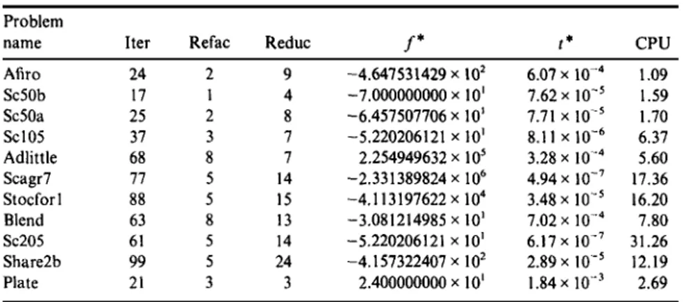
Table 1 . Solution statistics of LPPEN on the test set. Problem name Afiro Sc50b Sc50a Sc105 Adlittle Scagr7 Stocfor 1 Blend Sc205 Share2b Plate Iter 24 17 25 37 68 77 88 63 61 99 21 Refac 2 1 2 3 8 5 5 8 5 5 3 Reduc 9 4
f*
-4.647531429 x 10² -7.000000000x10² 8 -6.457507706x101 7 7 14 15 13 14 24 3 -5.220206121 x 101 2.254949632 x 10⁵ -2.331 389824 x106 -4.113197622x10⁴ -3.081214985x101 -5.220206121 x 101 -4.157322407 x10² 2.400000000x101 t* 6.07 x 10-4 7.62 x10⁻⁵ 7.71 x 10⁻⁵ 8.11x10- 6 3.28x10- 4 4.94 x 10⁻⁷ 3.48 x10⁻⁵ 7.02 x10⁻⁴ 6.17 x 10⁻⁷ 2.89 x10⁻⁵ 1.84 x10⁻³ CPU 1.09 1.59 1.70 6.37 5.60 17.36 16.20 7.80 31.26 12.19 2.69To initiate the algorithm, we choose a starting point y0 and t0 as follows.
We let y0 be a solution to
where ke(0, 1). Then, t0 is chosen using the following formula:
where Be(0, 1), r0 = ATy0 + c, and MINRES is a function that returns the mth
smallest element of r0.
4.2. Test Results. We consider ten problems from the Netlib collec-tion. We also used a test problem from a civil engineering application at the Technical University of Denmark, referred to as Plate. The characteristics of the test problems can be found in Ref. 1. We do not use any preprocessing on the test problems prior to solution. In Table 1, we show the solution statistics of the LPPEN. The tests were performed on an IBM PS/2-486. The Salford F77 compiler was used. The columns Iter, Reduc, and Refac refer to the number of iterations, number of reductions of the parameter t, and number of refactorizations. The columns f* and t* report the objective function value reported on termination and the final value of t, respectively. Finally, we report the solution time in seconds exclusive of input/output under CPU. We stop when
and the largest negative component of the residuals r = ATy + c is less than n||c||ooeM in absolute value, where eM denotes the computer unit roundoff. In connection with the initialization, we used K = B = 10-1 for all the
varies in the range between O(10- 7) and O(10-3), the penalty algorithm
yields very accurate optimal solutions. This is a very encouraging result, since quadratic penalty function methods have been well known for their potential numerical instability. These experimental findings corroborate our analytical results that the penalty parameter t is decreased to zero in a well-conditioned manner by solving a linear system of equations and taking a step along the solution.
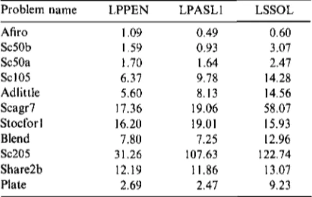
In Table 2 below, we provide a comparison of LPPEN with LPASL1 and LSSOL. We consider only the solution time in CPU seconds. For details on the results of LPASL1 and LSSOL, the reader is directed to Ref. 1. These results were obtained on the same computer under identical compiler settings. The results of Table 2 clearly demonstrate that, on the test set, LPPEN and LPASL1 display very similar numerical performances. Both codes also deliver a solution in times competitive with LSSOL.
4.3. Relation to Interior-Point Methods. Interior point methods solve a weighted least-square system of the form
Table 2. Comparison of solution times for LPPEN, LPASL1, and LSSOL on the test set. Problem name Afiro Sc50b Sc50a Sc105 Adlittle Scagr7 Stocfor1 Blend Sc205 Share2b Plate LPPEN 1.09 1.59 1.70 6.37 5.60 17.36 16.20 7.80 31.26 12.19 2.69 LPASL1 0.49 0.93 1.64 9.78 8.13 19.06 19.01 7.25 107.63 11.86 2.47 LSSOL 0.60 3.07 2.47 14.28 14.56 58.07 15.93 12.96 122.74 13.07 9.23
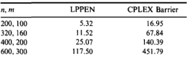
where D is diagonal positive-definite matrix and p,f are vectors of appropri-ate dimensions. Since the numerical values of the entries of D change from one iteration to the next, a numerical refactorization of the matrix ADAT is performed at each iteration of these methods. However, we do only occa-sional refactorizations of the matrix AWAT. As a preliminary test, we ran some randomly generated dense problems to force CPLEX to use dense linear algebra on a SUN SPARC 4 using the CPLEX Barrier optimizer and
Table 3. Comparison of solution times for LPPEN and CPLEX Barrier optimizer on dense problems on a SUN SPARC 4 (25 MHz). n, m 200, 100 320, 160 400, 200 600, 300 LPPEN 5.32 11.52 25.07 117.50 CPLEX Barrier 16.95 67.84 140.39 451.79
LPPEN. The results are given above in Table 3. The times are in CPU seconds.
These results clearly show that LPPEN is well suited for dense problems. In the light of the observations, we believe that the penalty method deserves further research.
References
1. MADSEN, K., NIELSEN, H. B., and PINAR, M. C., A New Finite Continuation Algorithm for Linear Programming, SIAM Journal on Optimization, Vol. 6, pp. 600-616, 1996.
2. MANOASARIAN, O. L., Normal Solutions of Linear Programs, Mathematical Programming Study, Vol. 22, pp. 206-216, 1984.
3. MADSEN, K., and NIELSEN, H. B., A Finite Smoothing Algorithm for Linear l1-Estimation, SIAM Journal on Optimization, Vol. 3, pp. 223-235, 1993. 4. HUBER, P. J., Robust Statistics, John Wiley, New York, New York, 1981. 5. MADSEN, K., and NIELSEN, H. B., Finite Algorithms for Robust Linear
Regres-sion, BIT, Vol. 30, pp. 682-699, 1990.
6. BERTSEKAS, D. P., Necessary and Sufficient Conditions for a Penalty Method to Be Exact, Mathematical Programming, Vol. 9, pp. 87-99, 1975.
7. MANOASARIAN, O. L., and MEYER, R. R., Nonlinear Perturbations of Linear Programs, SIAM Journal on Control and Optimization, Vol. 17, pp. 745-752, 1979.
8. Li, W., PARDALOS, P., and HAN, C. G., Gauss-Seidel Method for Least-Distance Problems, Journal of Optimization Theory and Applications, Vol. 75, pp. 487-500, 1992.
9. Li, W., and SWETITS, J., Linear l1-Estimator and Huber M-Estimator, Technical Report, Old Dominion University, Norfolk, Virginia, 1995.
10. MICHELOT, C., and BOUGEARD, M., Duality Results and Proximal Solutions of the Huber M-Estimator Problem, Applied Mathematics and Optimization, Vol. 30, pp. 203-221, 1994.
11. GILL, P. E., HAMMARLINO, S., MURRAY, W., SAUNDERS, M. A., and WRIGHT, M. H., User's Guide for LSSOL (Version 1.0): A Fortran Package for
Con-strained Linear Least Squares and Convex Quadratic Programming, Report
SOL 86-1, Department of Operations Research, Stanford University, Stanford, California, 1986.
12. BARTELS, R. H., A Penalty Linear Programming Method Using Reduced-Gradient
Basis-Exchange Techniques, Linear Algebra and Its Applications, Vol. 20,
pp. 17-32, 1980.
13. CONN, A. R., Linear Programming via a Nondifferentiable Penalty Function, SIAM Journal on Numerical Analysis, Vol. 13, pp. 145-154, 1976.
14. CHEBOTAREV, S. P., Variation of the Penalty Coefficient in Linear Programming
Problems, Automation and Remote Control, Vol. 7, pp. 102-107, 1973.
15. CLARK, D. I., and OSBORNE, M. R., Finite Algorithms for Huber's M-Estimator, SIAM Journal on Scientific Computing, Vol. 7, pp. 72-85, 1986.
16. DAX, A., Linear Programming via Least Squares, Linear Algebra and Its Applications, Vol. 111, pp. 313-324, 1988.
17. PINAR, M. C., Linear Programming via a Quadratic Penalty Function, Zeitschrift fur Operations Research, Vol. 44, pp. 345-370, 1996.
18. LUENBERGER, D., Linear and Nonlinear Programming, Addison-Wesley, Reading, Massachusetts, 1984.
19. NIELSEN, H. B., AAFAC: A Package of Fortran 77 Subprograms for Solving
ATAx = c, Report NI-90-11, Institute for Numerical Analysis, Technical