τ κ
S/OZ
-3
■АЗЗ
1337
-ш т е і-ш -ш м в ^ -ш > м ж ^ х г -ш зас-ш ю м
a r f í i s s
MESPÎêîaS 3*üjT3iEE-la ^Г'Г ρ-. .f iirr-i' B íJ B M rm sD ІЮ TJ33¡ jij>m Ί- ш ш в т ю ш -с^ . ¿ .ж . ■ O F ш г т т а з ж " T J 'S . t ΌΛ'ΓΓΛ.ΪΤ. ' ¡ π * · Γ ~ · · . · · ' Τ ί Г .’ГІ ί-.·"··Τ·: Τ-;ΤΤ-Λ;:r "·■=.,-Γ·' .ΤΓ>,<ϊ",ν;,· *♦/Т ^ Г. i'*·.·REGRESSOR BASED ADAPTIVE INFINITE IMPULSE
RESPONSE FILTERING
A THESIS
SUBMITTED TO THE DEPARTMENT OF ELECTRICAL AND ELECTRONICS ENGINEERING
AND THE INSTITUTE OF ENGINEERING AND SCIENCES OF BILKENT UNIVERSITY
IN PARTIAL FULFILLMENT OF THE REQUIREMENTS FOR THE DEGREE OF
MASTER OF SCIENCE
By
Emrah
ACAR-CjcaT
τ κ
б Ч о і . Э ■ <\ΖΖ
I certify that I have read this thesis and that in iny opinion it is Fully adequate, in scope and in quality, as a thesis for the degree of Master of Science.
/a fu h L
Assist. Prof. Dr. Orhan Arikan(Supervisor)
I certify that I have read this thesis and that in iny opinion it is fully adequate, in scope and in quality, as a thesis for the degree of Mcister of Science.
Prof. Dr. Erol Sezer
I certify that I have read this thesis and that in niy opinion it is fully adc in scope and in quality, as a thesis for the degree of Master of Scic'uce.
A i ^ c . Prof. Dr. O m e/M orgiil
Approved for the Institute of Engineering a.nd Sci('iic('s:
A / J ,
Prof. Dr. Mehmet B ^ y
ABSTRACT
REGRESSOR BASED ADAPTIVE INFINITE IMPULSE
RESPONSE FILTERING
Emrali AGAR
M.S. in Electrical arid Electronics Engineering
Supervisor: Assist. Prof. Dr. Orlian Arikan
July 1997
Superior performance of fast recursive least squares (RLS) algorithms over the descent type least mean square (LMS) algorithms in the adaptation of FIR systems lias not been realized in the ¿idaptatioii of IIR systems. This is because of having noisy observations of the original system output resulting in signiiicantly biased estimates of the system parameters. Here, we propose an adaptive IIR system structure consisting of two |)arts: a two-channel FIR adaptive filter whose parameters are updated by a. RLS type algorithm, and an adaptive regressor which provides more reliable estimates to the original system output based on previous values of the adaptive system output and noisy observation of the original system output. Two diflerent regressors are investigated and robust ways of adaptation of the regressor parameters are proposed. The performance of the proposed algorithms are compared with successful LMS type algoritlims and it is found that in addition to the expected convergence speed up, the proposed algorithms provide better estimates to the system parameters at low SNR value. Also, the extended Kalman filtering approach is tailored to our application. Comparison of the proposed algorithms with the extended Kalman filter approach revealed that the proposed approaches provide itiijiroved estimates in systems with abrupt parameter changes.
Keywords: Adaptive IIR Filtering, ARX, RLS, Kalman Filtering
ÖZET
DOĞRULTUCU TABANLI UYARLAMALI SONSUZ İTMELİ
SÜZGEÇLEME
Emrah ACAR
Elektrik ve Elektronik Mühendisliği Bölümü Yüksek Lisans
Tez Yöneticisi: Y. Doç. Dr. Orlicin Arıkan
Temmuz 1997
Sonlu itmeli (FIR) süzgeçlerdeki hızlı ÖEK (RLS) algoritmaia.rmın EOK (LMS) al goritmalarına göre olan üstün performansları, sonsuz itmeli (IIR) süzgeçlerin uyarla masında henüz yer almamıştır. Bunun nedeni uyarlamah süzgeçteki pürüzlü referans
dolayısıyla sistem parametrelerinin yanlı olarak kestirilebilmesidir. Bu çalışmada, iki
kısımdan oluşan bir uyarlamalı sonsuz itmeli süzgeçleme yapısı önerilmiştir: İlk kısım, dönüşüm temelli çok kanallı en küçük kare köşegen yapısındaki (JR-MESL aigoritmasıyla uyarlanan iki kanallı sonlu itmeli süzgeç; ikinci kısım ise uyarlayan sistem sonuçları ve orjinal süzgecin pürüzlü referansları ışığında, gözlenemeyen gerçek referansın kestiriminde bulunan bir doğrultucudan oluşmuştur, iki farklı tip doğrult ucu incelenmiş ve doğrult ucu parametrelerinin dayanıklı belirlenme yollan önerilmiştir. Önerilen algoritmaların, bilinen metodlarla karşılaştırılması yapılmış ve yakınsama hızındaki artışın yanısıra düşük sinyal gürültü durumunda daha doğru kestirimler elde edilmiştir. Ayrıca genişletilmiş Kalman süzgeçleme yöntemi probleme uyarlanmıştır. Önerilen doğrult ucu temelli algoritmalarla, genelleştirilmiş Kalman süzgeçlemenin karşılaştırılmasında, ani değişim göstei'en sistem lerin tanımlanmasında önerilen algoritmaların daha yüksek başarımı olduğu gözlenmiştir. Anahtar Kelimeler: Uyarlamalı süzgeçleme. Kalman süzgeçleme, ÖEK (RLS) algorit ması
ACKNOWLEDGEMENT
I would like to express my deep gratitude to rny supervisor Assist. Prof. Dr. Orhan Arikan lor his guidance, suggestions and valuable encourcigernent throughout the development of this thesis.
I would like to thank Prof. Dr. Erol Sezer and Assoc. Prof. Dr. Ömer Morgül for reading and commenting on the thesis and for the honor they gcive me by presiding the jury.
I am also indebted to my family for their pcitience and support.
Sincere thanks are also extended to every close friends who have helped in the development of this thesis.
Contents
1 Introduction 1
2 H R System Model and Proposed Adaptive HR Filter Structure 4
2.1 IIR System M o d e l... 4.
2.2 A Regressor Based IIR Adaptive Filter Structure 5
3 Proposed Regressors 8
3.1 IIR —7 A lg o r it h m ... 8 3.2 IIR-Kalrnan A lg o r ith m ... 10
4 System Identification by Extended Kalman Algorithm 15 5 Simulation Experiments 19
.'j.l Simulation Example 1 20
.5.2 Simulation Example 2 22
.5.3 Simulation Example 3 23
6 Conclusions and Future Work 28
CONTENTS Vll
A An Efficient Method of Estimation of var(u(n)) 30 B Two-Channel Lattice Structure of an H R Filter 33
List of Figures
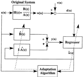
2.1 Common structure o f Illi—'y and nil-Kalm an adaptive systems.
3.1 Some example functional relation between L{n) and 7,,,; (a) = 0.1,/2 = 0.8, K = 0.5,p = 2, (b) h = 0.1,/2 = 0.8,«: = 0.5, p = 1, (c)
/1 = 0.2, /2 = 0.7, K = 0.75, p = 2, (d) k = 0.2, k = 0.7, k = 0.25, p =
2 ... 11
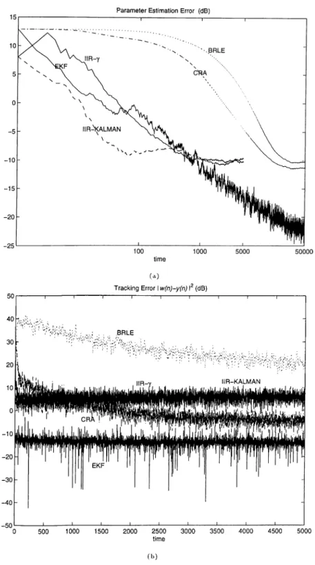
5.1 Results o f first example: (a) squared norm o f parameter error as a function o f time. Logarithmic time axis is used to resolve early convergence behavior o f the algorithms, (b) output tracking error
||t/;(72) — y{n)W^ as a function o f time. 24
5.2 Bar chart o f squared parameter error norm in dB at convergence of the algorithms at different noise levels for Example i 25 5.3 Bar chart o f squared parameter error norm in dB ¿it convergence o f the
regressor algorithm when the mixing pcirameter, 7,1, is kept constcint during the iterations for Example 1. Cori'esponding Vciricincc o f the output noise is 0.25. Note that the marginal OE ¿ind EE formulations have larger error levels, than a compo.sed regressor. 25 5.4 Results o f second example: squared norm o f the p¿u'a■meter error ¿is
a function o f time when the par¿ımeters o f the origimil system ¿ire abruptly changed at time 500... 26
LIST OF FIGURES IX
5.5 Results o f third example: the original system pcirameters are abruptly changed at time 400, (a) squared norm o f parameter error as a func tion o f time, (h) output tracking error ||t«(?'i) — y{n)\\^ as a function
o f time. 27
List of Tables
3.1 Equations o f IIR-Kalman State E s tim a to r ... 13
3.2 QR-MLSL Algorithm and Parameter Identification in the
Two-Channel Lattice Form 14
4.1 Equations o f General Extended Kalman Algorithm 17
4.2 Equations o f Extended Kalman Algorithm Applied in Adaptive HR, F ilterin g ... 18
h.l Equations o f Bias-Remedy Least Mean Square Equation Error Algo rithm (B R L E )... 19
.5.2 Equations o f Composite Regressor Algorithm (CRA) 20
5.3 Squared parameter error norm in dB at convergence o f the algorithms at different noise levels for Example 1 ... 22
Chapter 1
Introduction
Adaptive filters have found widespread use in nicuiy different signal processing ap plications where there is no reliable prior information on the system parameters or the parameters vary in time. Mainly because of its simplicity in implementations, a Finite Impulse Response (FIR ) system structure is usually preferred for the adap tive fdter. However, the choice of FIR structures severely limits the performance of the adaptive filters when the required adaptation necessitates the use of fitters with poles as well as zeros. However, even in these cases, the natural choice o f using an adciptive filter with Infinite Impulse Response (HR) structure has not Ibund much room in applications. The m ajor reason behind this fact is the lack of HR adapta tion algorithms which robustly converge to the desired system parameters in a short time. The trade-off between the convergence and bias of the estimated system parameters has been the subject matter of many investigations on HR adaptcition approciches [1- 6].
There cire two main approaches to adaptive HR filtering, based on two different definitions of the error sequence which is iteratively tried to be minimized by the cixlaptation algorithm. In the output error formulation, the error seipience is defined as the difference between the desired and the output sequences of an HR filter whose parameters are adjusted iteratively by the adaptation algorithm. Altliough, the output error formulation is a very natural extension of the FIR adaptation concept, unlike the FIR Ccise, the weighted least sqiuu’es cost function is no more quadratic with respect to the adaptive HR system parameters. This limits us to use
Chapter 1. Introduction
slowly converging gradient descent adaptation techniques wliicli is not acceptable especially for systems whose parameter changes faster than the convergence of the adciptive system. Furthermore, the cost surface may have com plicated local minima structure making it very difficult for the gradient descent algoi'ithms to converge to the globally optimal HR system parameters. Also, stability monitoring becomes a critical issue in the output error adaptation. Mcuiy of the difficulties of the output error formulation do not exists in the equation error formulation where tlie error sequence is defined as the difference between the desired secpience and tlui output of a two-channel FIR filter whose inputs are the avaihible input sequence and one-sam ple delayed desired output secpience. Since the corresponding weighted least squares cost function is quadratic with respect to the two-channel FIR filter parameters, fast recursive least scpiares adaptation algorithms can be used to obtain the globally optimal system parameters. However, even in the sufficient order modeling, when there is an additive measurement noise in the desired sequence, the obtained results are biased estimates of the unknown system parameters.
In order to capture the beneficial features of the equation error Idinnidation and reduce the bias in the converged parameters, various bias remedy approaches have been pi'oposed [2 -4 ,6- 8]. In some of these apiaroaches the error sequence is defined as a convex combination of the equation and output error se(|uerices [.'5]. Then, the lecist squares cost function is tried to be minimized by using a gradient descent algorithm based on the instantaneous gradient estimate. It has been shown that witli a judicious choice of the convex combination parameter, significantly more accurate parameter estimation can be achieved [2,3]. However, because of the use of an update strcitegy based on instantcuieous gradient estimate, the speed of convergence of these algorithms is slow.
In this thesis, we propose cin adaptive HR system structure consisting of two parts: a two-channel FIR adaptive filter cind an adaptive regressor wliich provides more relicible estimates to the original system output. As shown in Fig. 2.1, the two-channel FIR adaptive filter has as its inputs the input of the original system,
x(n), and the delayed output of the regressor, iü(n), which is an estimate to the
original system output, io{n). This way, the parameters of the adaptive filter can
be updated efficiently by using a multi-channel recursive least squares algorithm such as Q R -M L S L [9,10]. We consider two different adaptive regressors to provide relicible estimates to the original system output causcilly based on adaptive system
Chapter 1. Introduction
estimate to w(n) as a convex combination of the y(n) and d(n), where the convex
combination parameter 7„ is adapted bcised on the convergence of the iterations. In
the cidaptation of 7„, the regressor performs 0 ( N ) multiplications where N is the
order of the adaptive system. In the second type of regressor, a simplified Kalman
filter is used to provide the estimate, w(n), to w{n), where the required state space
model of the system is obtained from the adiipted system. The required number of
multiplications of the Kalman regrssor is 0(N'^). In chapter 3, we investigate both
regressors and provide robust ways of adapting their parameters. Also in the same chapter, the steps o f the adaptcition algorithms for both regressors are tabulated.
In chapter 4, the well known extended Kalman filter algoritlim is tailored to our cipplication [11-13]. It is shown that since the resultcuit algorithm requires
no-m atrix inversions, system parameters can be estimated by com puting O(N^)
multiplications. Also, a robust way of updating the required covariance nuitrices is provided.
In chapter 5, we provide extensive comparison results between the approaches investigated in this work and earlier proposed approaches to HR adaptation [2,3, 12,13]. In chapter 6, we provide the conclusions of our work and address potentiell areas for future work.
Chapter 2
H R System Model and Proposed
Adaptive H R Filter Structure
2.1
H R System Model
As shown in Fig. 2.1, in ci typical adaptive filtering application, input, ;r(?7.), cUicl
noisy output, d(n), of an unknown system are a.vaila.bie for processing by an adap
tive system to provide estimates, y(n), to the output of tlic uuknown system as time
progresses. If the ultimate purpose is to keep tra.ck of the variation iu the uidaiowii system parameters, the required processing is called as adaptive syst(;m identifi- ca,tion. However, there cire many other important airplication areas of adaptive filtering such cis adaptive prediction, noise cancelling, echo cancelling and cliannel equalization, where the primary purpose is not the estimation of the unknowu sys tem parameters [5,14,15]. The approaches we will investigate in this thesis are generally iipplicable in all these cipplication areas.
In our investigation the unknown system or plant has an HR model whose; out|)ut can be com pactly expressed as a function of its previous vahuis and its input as:
N M
Chapter 2. HR System M odel and Proposed Adaptive HR Filter Struct'ucture 0
Figure 2.1: Common structure o f IIR—j and IIR-Kalman adaptive systems.
where 0 is the vector of direct form system parcimeters:
-tT
0 = «1 UN bo h 0M'M (2.2)
and (f>{n) is formed by the previous values of the output and the |;)resent and past
vcdues of the input:
-\T ^(n) = w{n — 1) · · · w(n)"^ x ( n y w{n — N) x(n) x(n — I) tT x(n - M ) (2.3) In the above relation, the system is assumed to be time-invariant. Tim e varying
systems can be m odeled with 6, which has time-Vcirying entries. Our a.im is to develop
adaptation algorithms tlmt can be utilized for both time invariant and tim e-varying systems. However, the variation of the system parameters should be either a. slow function of time, or else, cibrupt changes in the system parameters should occur infrequently in time.
2.2
A Regressor Based H R Adaptive Filter Structure
In FIR adaptive filtering, the model is a tapped-delay-line and only the in|)ut samples determine the output of the plant and the model. No Feedl)ack loop exists inside the
Chapter 2. HR System M odel and Proposed Adaptive HR. Filter Stractm■e
system and stability in BIBO sense is always assured. In adaptive HR filtering, due to the feedback existing in the system, we are faced with the problem of deciding on the feedback signal used in the adaptive system when we Imve noisy observations of the actual system output. Hence, as shown explicitly in Fig. 2. 1, we need a regressor that causally performs the required estimation of the feedback signal based on the
noisy output d{n) and the output of the adaptive filter y{n), which is obtained as:
y(n) = 0^ {n)^{n) (2.4)
where l ( n ) , the vector of estimated system parcurieters, can be written as:
0{n) =
tT
â i(n ) ··· âN{n) bo{n) bi(n)
iT
a(n)^ b (n )^
bmin)
(2.5)
and ^(n) is the vector of the regressor output, w{rt)^ and the system input, ;r(n):
¿(?r) = iT w(n - 1) io{n — N) x[n) x{n — 1) iT x{n - M ) w(?r)^ x(n)-' (2.6)
The performance of the adaptive filter heavily depends on how well tlie regressor
provides estimates to the actual system output to{n). The two well known formula.-
tions of adaptive HR filtering, namely the output error (OE) and the equation error (EE) formulations, correspond to two different types of regressors.
In the OE formulation, the vector ¿ ^ (n ) is described cis
¿ o ( « ) = y{n - 1) · · · ?/(n - N) ;c(??,) x{n - 1) ,'i;(?7, — M )
y { n f x(n)'^
iT
(2.7)
which corresponds to a regressor whose output is the output of the adaptive filter. In the EE formulation the signal vector, ¿^ (?i) is given as:
= -\T d { n - l) ■■■ d{n - N) x(n) x(n - 1) iT d(?7)^ x (n )^ x(n - M) (2.8)
Chcipter 2. HR System M odel and Proposed Adciptive HR Filter Structure 7
which corresponds to a regressor whose output is the noisy observation of the system
output, d{n) = w(n) + u(?r).
Since the least squares cost function of EE formulation is (piadratic in terms
of the parameter vector 0, fast converging recursive least s(|ua,r(;s t(H-.liniqu(is can
be used in the adaptation. However, because of the additive measuixmient noise,
v(n), the converged parameter values are bicised (estimates of the actual system
para.meters [7,16-18]. In the OE formulation, the least s(|uares cost function is not a quadratic function of the parameters. Hence, we are bound to use; LAdS type gradient descent techniques in the adaptation. When these LMS type adaptation algorithms converge to the global minima of the cost function, the obtained parameters are unbiased estimates of the cost function. Unfortunately, not only LMS type gradient adaptation methods converges slowly, but also, tliey may converge' to a local minima of the cost surfcice. Various algorithms have been proposed to combine the beneficial features of the OE and EE formalism in one algorithm [1 -4,G ,7,19]. Notably, the bias remedy least mean square equation error (BRLE) [2] and the com posite regressor algorithms (CRA.) [3] are proposed to obtain low biased parametcM· estimates by using gi’cidient descent type adaptation [11,16-18]. However, sincxe the corresponding cost functions o: these algorithms are not designed to b(; qua.dratic with respect to the parameters, recursive least squares techniques cannot Ix'. utilized to ol)tain fast converging estimates to the parameters.
In the first part of our work, we also try to coml)ine the desiix'd features of both OE and EE formalism in one formulation wlicire tlie cost function is kept as a quadratic function of the parameters. As suggested in Eig. 2.1, this is acliieved
by choosing the adaptive filter as a two-channel EIR filter with inputs x{n) and
iu(n — 1). Then, the corresponding weighted least squares cost function becornc.s:
A:=l
(2.9)
which is a qiuidratic function of 0, becciuse ^(n) is a. fixed sequence of vectors det<n·-
mined by the past parameter estimates &(n — — 2), · · · ,^ (0 ). Ih'iice, efficient
multi-channel FIR recursive leevst sejuares techni((ues can l)e used to obtain param
eter estimates ai time n, ¿ (n ), as the minirnizer of
In the following chapter, two different types of regn^ssors will be investigated in detail and corresponding recursive leivst squares adaptation algorithms wdll be presented.
Chapter 3
Proposed Regressors
The performance of the regressor based HR adciptation structure largely depends on how well the actual system output is estimated by the regressor in Fig. 2.1. In this chapter, we investigate in detail two types of regressors.
3.1
H R
—7
Algorithm
In the first class, the regressor output is estimated as a couv('.\ combination of the
noisy observations, d{n) and the adciptive filter output, y{n) as
u;(?r) = jnd(n) + (1 - 'jn)y{n)^i , 0 < 7„ < 1 (3.1)
where 'yj\s the regression coefficient. In the following, the HR adaptation algoritlnn
which uses this type of regressor is referred to as H R—7 .
The proper choice of 7,1 should be based on a measure of the reliability of tlie
estinicited system parameters. A significant deviation of y{n) from d{n) is a.n indi
cation that the system i^arameters are not reliably estimated, and heiuxi, 7,,, sliould be chosen close to 1, so that equation error type a.dapta.tion should tahe place. On the contrary, if y(n) closely follows d{n), then to reflect our level of confidence to the estimated system parameters, 7„ should be chosen close to 0, so that output error type adaptation should be performed. We propose to liase the measuix' of
Chapter 3. Proposed Regressors
reliability of the estimated system parameters to the statistical significcuice of the
observed deviation between ij(n) and d(n) sequences. For this purpose, one way
of choosing 7„ is based on weighted estimate o f the expected energy o f the error
sequence e(n) = d(n) — y{n):
L{n) = EILo - i f (3.2)
A* ’
where is an exponential forgetting factor that can im|:)rove the performance of the
estimator. In this approach, the regressor pcirameter 7,,, is aii increasing function ol L(n), because large values of L{n) is an indication of deviation from the true
system parcuneters. In our investigation, we observed that the critical properties of
the functional foi'm between L(n) and 7„ are the boundary values ly and /2 such
that 7„ = 0 if L{n) < ly and 7„ = 1 if L{n) > /2. In between these two boundaries,
various forms o f increasing functions can be used. In order to determine which
values for ly and /2 should be used, we investigated the expected value of the L[n)
for the cases o f 7« = 0 and 7„ = 1, which correspond to output and equation error adaptation cases respectively. Assuming that 7„ = 0 and the estimated parcurieters
have converged to the actual ones, the observed error sequence, e(n) will be equal
to v(?i), the additive Gaussian observation noise. Hence, the ('xpected value of Lin)
will be (Ty, the variance of v{n). Therefore, ly is chosen as a'l· Likewise, when 7„ = 1
and convergence of weights are established, expected value of L{n) is equal to the
variance o f e(n) sequence for the equation error formulation. Since equation error
e¿г(?г) is related to the output error eo{n) as [2]:
CEin) - eo{n) - a ' ( n ) e o ( ? 7 . ) . (3.3)
when '^(77) is white noise, the variance of eE{n) can be written as:
var (eEin)) == al j
at the time o f convergence to true pcirameters. Hence, we propose to use:
k = , k = Ua li l + J ] d · ) (3.5)
where [ / > 1 is introduced so thcit 7„ should not be kept fixed at I near tlui conver gence point o f the equation error adaptation.
Chcipter 3. Proposed Regressors 10
For computational efficiency, the actual form of functionaJ relation between L{n)
and 7„ is chosen as follows:
7n 0 Lin) < /, ÍI < t ( " ) < 4 ^ 1 - (1 - 4 ^ < U n ) < k (L(n)-h)v ^ fh-h (3.6) 1 L(n) > k
where k and p are two parameters providing some control of the actual shape of
the curve in between two boundaries l¡ and /2. Fortunately, we oirserved that the
Irehavior of the algorithm is not so sensitive to these slia|)e |:)ara.meters. I'or each
iteration, this regression algorithm requires ( N + 11) multiplications which is OiN).
Some examples of the above functional relation (3.6) Ccui be seen in Fig. 3.1 Ibr Vcirious shape parameters.
3.2
IIR -K alm an Algorithm
In the second class, we consider a Kalman regressor structure based on the [bllowing state space model of the origincil system [11-13,15]:
w( n + 1) = ^w (?r) + Bx(n) V (3.7)
din) - Cwin + 1) + vin) (3.8)
wtiere C = 1 0 and the state transition matrices are:
I A = -ÜI —«2 · · · —aN 1 0 0 0 1 0 0 1 0 B = bo by 0 0 bM 0 0 0 0 0 (3.9)
Since the actual parcirneters are unknown, we cannot use tlie state s|)a,ce model
Chcipter 3. Proposed Regressors 11
( a )
no
( c )
(^0
Figure 3.1: Some example functional relation between L{n) and 7„; (a) l[ = 0.1, /2
0 .8 ,/c = 0.5,p = 2, (b) h = 0 .1 ,/2 = 0.8, K = 0.5,p = 1, (c) h = 0 .2 ,/2 = 0.7, k
Chapter 3. Proposed Regressors 12
the estimated parameters at time n, we get the following state space model:
w (?2 + 1) = A ( n) w ( n ) + B{n):x.(n) + u(n) (3.10)
d{n) = Cw(i7, + 1) + u(?i) (3.11)
where u(n) is introduced as an additional noise term to the system clynamics to
account for the approximations in A and B by A{n) and B{n), which are equal to:
A { n) = —di{n) —({2(77) 1 0 0 1 0 1 —а^{п) 0 0 0 , B{n) = boin) 61(77.) 0 0 Ьм(п) 0 (3.12)
Since the approximation in ^ ( 77) and B{n) only limited to the first row, the addi
tional process noise u(7r) can be written as:
и(?г) =
tT
иin) 0 0 (3.13)
In order to apply Kalman estimator on the approxirna.te model given by Eqns. (3.10)
¿uid (3.11), we need the covariance matrices TZu{n) and 'Rv(n) of 77(77,) a.nd 77(77.)
respectively. In addition, we need an initial estirniite to the state vector w (0 ) 7uid
the variance o f the initial system error 7^„,(0). The covariance matrix ‘R-uin) is
determined by the variance ol u(n) lor which a robust way of fipproximation is
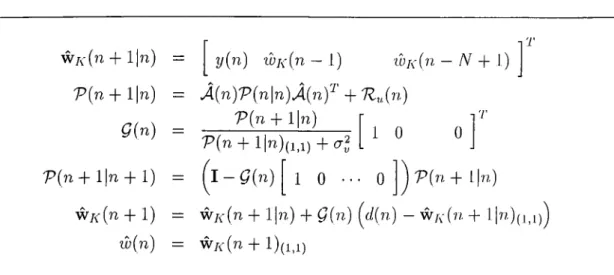
presented in the Appendix A. The steps of the corresponding Kalman estimator are given in Table 3.1, where A i n ) , B i n ) , w i n ) are defined in Eqns. (3.12), (2.6) and the
notcvtion of is used to denote the first dicigonal entry of the matrix T . Note
that the output of the regressor гЬ{п) is the first entry in the estinmted state vector
W/c(77 + 1) and also the a-priori state estimate w/c(77. -Ь 1|77.) is obtained efficiently by using the output of the adaptive filter and the previous states of the Kcilman filter. The actual forms of the matrices in the above algorithm C7ui l)e exploited for more efficient computation of the regressor output 7(7(77). For each iteration, tlic
Kalman regressor requires (ZN'^ + 2N) multiplications, hence it is O(N^). 'The HR
adaptation algorithm which uses this type of regressor is referred to as HR -Kalman. The required two-channel FIR adaptation can be efficiently performed by using Q R -M L SL algorithm which is a rotation-based multi-channel least squares lattice
Chapter 3. Proposed Regressors 13 w /i(n + l|7г) V (n + l|n) 0(n) V {n + l|i2 + 1) WA'(n + 1) w(n) y{n) lUK-in - 1) WK(n - + 1) A { n) V { n \ n ) A ( n y + TZuin) V{ n + l|?i) P (n + l|?i)(i,i) + 0-2 . iT 1 1 0 0 1 - G i n ) 1 0 ··· 0 ] V ( n + l\n)
WA-(?г + 1|??,) + Q(n) (^d{n) - WA'(n + · bO(i,i))
Wa-(?2 +
Table 3.1: Equations o f IIR-Kalman State Estimator
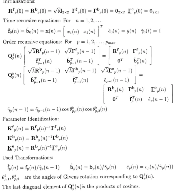
algorithm with many desired features [9]. The steps of this algorithm are given in
doable 3.2. For each update, this algorithm requires 0(4:N) multiplications. The
required direct form parameters for the Kalman regressor can be easily computed by using standard mapi^ing rules between lattice and direct form parameters [9]. The structure of multi-channel lattice FIR, filter and the mapping rule is explained in the Appendix 13.
Chapter 3. Proposed Regressors 14
Initializations:
Rf,(0) = R%(0) = ri‘p(0) = r ^ (0 ) = 02X, r , ( o ) = 0,2 X I
Tim e recursive equations: For = 1 , 2 , .. .
i T
fo(n) = bo(n) = x(?z) = Xl{n) X2{n) ¿o(n) = y(n) 7 o(0 = I
Order recursive equations: For p = 1 , 2 , .. .
Q p (« ) Qi (n) Rf,(·«.) ri',(77.) \/AR^p(?7 - 1) ^/XT^pin - 1)
fJ-iW
\ /A R ^ ( ? 7 - 1 ) ^/XT^p(rı-l) \ /A r « ,,( ? 7 - 1)b j_ i(n -l)
i p - i H
ep_i('n-l)
Rbp(,7) r^(77.) r p ( n ) -0
0'^' 7p(?7 - 1) = % - l ( n - 1) cos Ol^in) cosPcU’cuneter Identification: Kfp(?7) = R fp (7 7 )-'ri;(?7 ) Kbp(i7) = R ^ (? 7 )-lr % (7 7 ) K % { n ) = R \ (?7 )-lr% (7 7 ) Used Transformations:
fp(n) = fp(n)/7,(n - 1)
bp(n) = b j n ) / % { n )
i^(n) = c„{n)l%,{n))
> W > U are the angles of Givens rotcition corresponding to Qp(n)·
The last diagonal element of Qp(?7)is the products of cosines.
Table 3.2: QR-MLSL Algorithm and Parameter Identihcation in the Two-Channel
Chapter 4
System Identification by
Extended Kalman Algorithm
We propose the regressor based RLS algorithms for their potential of providing
more reliable feedback signal w{n) in the presence of output noise. In the IIR -
Kalman algorithm, a boot-strap method is used for an alterimting estimation of the system output and its parameters. The Kalman regressor |)rovides estimates to the noise free output, and then an RLS type adaptation procedure first updates the adaptive system parameters and then compute the output of tlie adaptive system,
y{n). As discussed in [11-13], these two stages of the adapta.tion can be combined
into one in an augmented stcite space description of the system. This approa.ch has been proposed for combined state estimation and tracking of slowly varying system parameters once a close initial estimate to the system parameters is available [12,13]. In this chapter, we provide the augmented state space description corresponding to HR cidaptive filtering and then derive the corresponding extended Kalman algorithm for the estimation o f the cuigrnented state. Also, we use a robust method, wliicli is presented in the Appendix A, for the choice of the required cova.riance matrices.
Chapter 4. System Identihcation by Extended Kalman Algorithm 16
The augmented state space description which will be exploited lor joint estima tion of the system output and its parcimeters is given as;
w(?r + 1)
6{n
+ 1)
.Â(?г)w(?г) + B( n)x{n) 0 ( n )+
u(?7,) S(?7,) (4.1)with the corresponding observation model of:
d{n) = r 1 w ( n - b 1 )
c
o ' · ^ L JQin
+ 1 ) .+
v{n).
(4.2)Here, u(?7) is the noise sequence vector on the output estimates, which we call cis
process noise as in IIR-Kalm an framework, cind s(n), which is assumed to be un-
correlcited with u(?7), is the noise vector on the pcirameter updates. Since ^ (?i)w (?r) involves multiplication of augmented state variables, extended Kalman filter cilgo- rithrn should be used in recursive estimation of the augmented state variables.
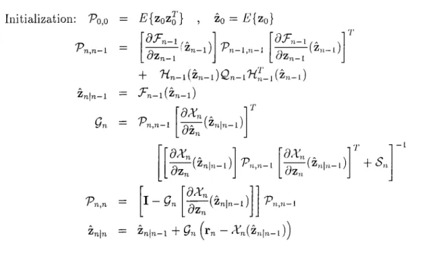
For the following general state sjDace model, the extended Kalman filter has been proposed for efficient estimation of the state
Zn+l = J^n(Zn) + (4.3)
r„ = XniZn) + (4.4)
where iFn and cire vector-valued functions and Tin is «i· matrix-valued function
with continuous first-order partial derivcitives. In the case of zero mean uncorrelated
Gaussian noise sequences, and rj , with
= QkHk - /) , = SkSik - /) ,
1%
z ^ } = 0 VA:,/ (4.5)
the steps of the extended Kalman filter algorithm are given in Table 4.1, as it was derived in [12].
This general form o f the extended Kcilman filter can be specialized to our appli cation by using the following substitutions:
Zn
= [ w(?z)^
0{n)^
, r„, = din]T/'
^n(Zn) = ^^(?7)w(?r) -)-H(?7)x(?7)y (n) > Tin{Zn) — l (4-6) Xn{zn) = Cw{n) , f = U(?7)^ S (n y T , ■// = n(77,).Chapter 4. System Identification by Extended Kedrnan Algorithm 17
The steps of the corresponding algorithm, that will be referred to a,s EKF, is given in Table 4.2. As seen from this table, the initial estimates of the states, the covariance matrices of the initial state estimate, the system and observation noises are required.
A robust way of approximating the covciriance matrix 7Zu{n) is presented in the
previous chapter and the Appendix A. Since the matrices have special structures, we can simplify the required comi^utatioiicd com plexity of the EKF. For instance,
both u(?r) and the observation matrix Ims only one non-zero entry, simplifying the
vector-m atrix operations. Hence, no matrix inversion is required in our application.
For each update, the EKF algorithm requires (12N'^ + 3/V/^ + 12 N M + 17N +
9 M + 4) multii:)lications which is an order more than that of IIR —7 and iiround 9 times more than that of IIR-Kalm an algorithms.
Initialization: Vop 'P n ,n -V Zn|n—1
Qn
= E {zqzI ] , Zo = /'.'{zo}dJ^n-i
<9z„_idTn-i
dzn-i
+ T i n- 1{ i n - l ) Q n - l T-Cn-1 ( z „ _ 1) •Fn.—l(Zn—1) dXn (Z n -l) = 'P n ,n -1 ^ T di. '(Z)i|n—1) \ d X n , .J
T T’n.ji-l (z„|„,-l) d z n + S n -1 'Pn,n —dXn
dzn
(Zn|n—1)V;
n,n—\. — Zfi|,i,_i T Qn ^n{Zn\n—l)'jTable 4.1: Equations o f General Extended Kalman Algorithm
In the following chapter, we provide extensive comparison results between the presented algorithms and LMS type regression algorithms: C R A and BRLF.
Chapter 4. System IdentiRcation by Extended Kahmin Algorithm 18 Initialization: w (0 ) ¿ (0) w (n + l|n) ¿(n + 1|?2)
£’{w(0))
¿ (0) ^(72)w(n) 0{n), no|o) =
TZ-w (0) 0 0 -RojO) + B( n)x{n) 0 V { n y - l\n) = J{n)V{n\'n)J{nY -\- Ru{r>) 0 0 Ro{ri) J ( n ) = A{n) 0 0 0 f-M+N+l Q { n ) --V { n4 - l \ n + l) = [1 — Q{n) V{ n + l|?i) (P (? 2 + + (t2) . 1 0 0 1 0 ) n n + l|r0 w{ n + 1) w (n + l|?i) £(n + 1) ^[n + l|?i) + Q{n) [din] - w (n + l|?i.)(u))Eli-Chapter 5
Simulation Experiments
In order to compare the regressor based feist RLS algorithms proposed in chapter 3 and the EKF algorithm discussed in chapter 4 with the earlier proposed gradient descent IIR adaptation algorithms BRLE [2] and CR A [3], their performances over synthetically generated examples are given in this chapter.
The steps of BRLE and CR A algorithms are given in Table 5.1 and Table 5.2.
eo (n )
eE{n)
ai{n +
1)
bj(n + 1)
Rem edy Parameter:
d(n)
-di{n) + ixtE{n) [d{n - i) - TCo{n - ·/)] i = 1, 2, bi(n + 1) + i.ieEin)x(n - j ) j = 0, 1, · · ·, M
0 < T < 1
determined by r = rnin(A: .J , I)
eo(n)
,
N
Table 5.1: Equations o f Bias-Remedy Least Mean Square Equation Error Algorithm
(BRLE)
For the required m ulti-channel RLS adaptation of the system parfimeters in the regressor based algorithms, rotation-based multi -channel least squares lattice algo rithm (Q R -M L S L ) given in Table 3.2, is used [9]. By using simple transformation
Chapter 5. Simulation Experim ents 20
w(?2)
kn)
e(n)
k n
+ 1)
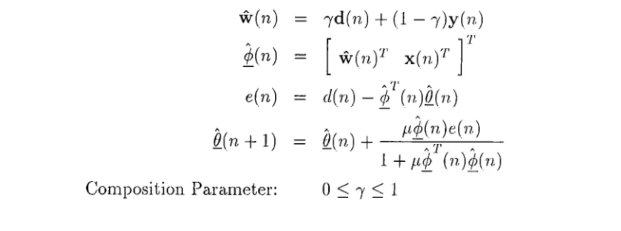
Com position Parameter;7d(??,) + (1 - 7 ) y ( « )
l'7'
w(n)^ x(?7,)’^’ d(n) — ^ (n)^(ri)y;4(77,)e(??.)
=
0(n)
+
T . 1 + {n)^(n)0 < 7 < 1
Table 5.2: Equations o f Composite Regressor Algorithm (CRA)
rules, the direct form parameters Ccin be obtained irom the reflection matrices of the cidapted two-channel FIR lattice filter [9]. In the following results, the parameter error vectors are com puted as:
eo{n) - 9_-0{r^)
where 0 is the actual and 0_[n) is the estimated direct form pa.rameters.
The cidaptive filters are “all-zero” initialized during each experiment. The sta tistical results com e from the the ensemble average of 50 realizations.
5.1
Simulation Example 1
In this first example, the same LTI second order IIR. system analyzed in [2,19] is used in cl system identification application. The traxisfer function of the original system is:
H{ z) =
1
(.5.2)1 - 1.7z-^ + 0.722.5.?-'·^'
The input sequence is a unit-variance white Gcuissian process. 'I'he output noise
process, v(n), is chosen as white Gaussian noise process. The output noise varicince
is varied to investigate the sensitivity of the performance of the algorithms to the level of SNR.
In P’ig. 5.1, the squared norms of the parameter error vectors, ||efy(';i.) corre
Chapter 5. Simulation Experim ents 21
deviation of the output noise, cry is set to 0.5. The forgetting factor A of the Q R -
MLSL algorithm is chosen as 0.999, and the parcimeters of the regressor subsystem
of Eqns. (.3.5) and (3.6) are chosen as A„ = 0.9, p = 1,a: = 0.7, fJ = 2. For the
IIR-K alm an regression cilgorithm, the initial variance estimate, al{0) is chosen as
unity cind the smoothing factor, /3 is chosen as 0.9. The EKF algorithm has cilso initialized with all-zero initialization for the augmented state vector with the same smoothing factor and unit 5-^(0) as well cis the dia.gonal entries o f the covariance
matrix 7io{0). In order to better resolve the Ccirly convergence behaviors of the
com pared algorithms, a logarithmic time axis is used in Fig. 5.1. As seen from this figure, the proposed algorithms have converged to an error level of -10 dB eiirlier than the 1000^^* Scimple, but the LMS type algorithms converge to the sa,me error level at about 40000*^'' sample. EKF algorithm, performing the best, converges to -20 clB at around 50000*^ sample. Here, the same step-size of 0.0005 is used for the CR A and BRLE algorithms. As recommended in [2] and [3], the com position parameter 7 for CR A is chosen as 0.9, and the remedier parameter of BRLE, r(?i) is chosen as m i n ( j i ^ ^ , 1).
Although the corresponding results of RLS equation error and output error adap- tcition are not shown in Fig. 5.1, they converged to error levels of -7 dB and 5 dB respectively, which are significantly higher than those of compared algorithms here. Therefore, as initially expected, the performance of the regressor based RLS ap- pi'oaches can be better than both the equation and output error formulations.
The tracking errors plot, ||in(n) — y{n)\\^ of the compared algorithms are shown
in Fig. 5.1. EKF and CR A algorithms have lower tracking errors, but the proposed regressor algorithms have a very fast convergence.
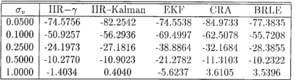
In order to compare the error on the parameters at the convei’gence of the a.lgo- rithms, we repeated this experiment at different noise levels. The obtained ||eii(??.)||^ results are given in Table 5.3 cind figured in Fig. 5.2. In this experiment the l)est performing algorithm is found as the EKF algorithm. However, EKF requires an or der more multiplications than H R —7 algorithm. As seen from these results, at high SNR (low levels of cr„), LMS type cilgorithms converge to lower error levels. Howev(M·,
as the SNR decreases (high values o f Uy) the proposed aigorithms start providing
closer or better results than LMS type algorithms, which is ¿m important cidva.ntage in many practical applications. Note that, the tabulated results correspond to the error levels at the 5000^^ sample for the proposed algorithms and 50000'^' samples
Chapter 5. Simulation Experim ents 22
lor the EKF, C R A and BRLE algorithms. Since, in many important applications, the speed o f convergence is very critical, the proposed algorithms provide a good trade-off between error levels and the speed of convergence even at high SNR. Also, IIR - 7 provides comparable results to IIR-K alm an although it requires an order less number o f multiplications.
(J V IIR - 7 IIR-Kcilman EKF GRA BRI.E
0.0500 -74.5756 -82.2542 -74..5538 -84.9733 -77.3835
0.1000 -50.9257 -56.2936 -69.4997 -62..5078 -.55.7208
0.2500 -24.1973 -27.1816 -38.8864 -32.1684 -28.38.55
0.5000 -10.2770 -10.9023 -21.2782 -11.3103 -10.2322
1.0000 -1.4034 0.4040 -5.6237 3.6105 3.5396
Table 5.3: Squared parameter error norm in dB at convergence o f the algorithms at
different noise levels for Example 1
5.2
Simulation Example 2
In this example, the performance o f the algorithms are comjrared when there is an abrupt change in the system pariimeters. For this purpose, we used the following tim e-varying transfer function for the original .system:
H { z , n ) Q.2759+0.5121;г~^+0.512L·‘;-'-^+0.2759.?-'^ ^ r n n l - 0 . 0 0 1 ; j - l + 0 . 6 5 4 6 ; ^ - ^ - 0 . 0 7 7 5 . ~ - ^ ’ ^ 0 . 7 2 4 1 + 0 . 4 8 7 9 ^ - ^ + 0 . 4 8 7 9 . ? - ^ 1 + 0 . 0 0 1 ^ - 1 + 0 . 6 5 4 6 ; ? - 2 + 0 . 0 7 7 5 ? n > 5 0 0 (h.3)
The input is chosen as zero-m ean unit variance white Gaussian process. Tlie output
noise v(n) is chosen as a zero-mecin white Gaussicui noise with a varia,nce of 0.25.
The step-size o f C R A and BRLE algorithms is set to 0.01, because a larger value for it would cause instability in the convergence. The com position parameter, 7 of GRA is set to 0.5, and the remedier parameter, r(?7.) o f BRLE is determined as in the first example. The forgetting factor of the proposed algorithms is set to 0.99 for a better tracking o f the variations in the system parameters. For IIR-Kalm an algorithm,
d-'iin) is chosen as unity and smoothing factor, fC as 0.9. 'I'lie pcira.meters of H R —7 in
Eqns. (3.5) and (3.6) cire cho,sen as = 0.95, p = 1,/i = 0 .3 ,// = 5. EKF algorithm
was also initialized with all-unit variances for all the elements in the state vector with the same smoothing factor of IIR-Kalmcin. In Fig. 5.4, ||eii(?7.)||·^ of each algorithm is shown. As seen from the.se results, both CR A and BRLE, whose performance are
Chcipter 5. Simulation Experim ents 23
very close to each other, are outj)eriormed by the proposed algorithms. 1111,—7 and IIR—Kalman have the best performance where EKF algorithm has converged to a higher error level. This is an expected result in the light of the first experiment where the convergence speed of the proposed algorithms were found as significantly faster than BRLE and C R A algorithms. Again, at an orderless amount of multiplications, IIR —7 provides comparable results to IIR-Kalnm n.
5.3
Simulation Example 3
In this example, the performance of the proposed regressor algorithms cue compared with the output error and equation error regressors when there is an abrupt change in the system as in the previous example. The tim e-varying system transfer function o f the simple one-pole system:
E ( z , n ) = 1 1 + 0 . 9 8 ^ t n < 400 n > 400 (5.4) l-0.98.r-i
The input sequence is chosen as in the second example. The output ■w(n) is dis
turbed liy a zero-m ean white Gaussian noise process with a„ = 3. 3'lie parameters
o f the regressor based algorithms are set as in the second example except the forget ting factor of the adaptation algorithm A, which is chosen as 0.95. 'The output error and equation error regressor methods are also cornlrined with the same adaptation algorithm, Q R -M L SL, with the scvme forgetting factor. The corresponding ||eii(?i)||'^ perlbrmance cuid the tracking performance, ||iy(n) — ?/(n)||^ of each algorithm are shown in Fig. 5.5.a and Fig. 5.5.b. The shown results a.re ensemble averages of 250 realizations. As seen from Fig. 5.5.a, the proposed regressor algorithm provide more reliable estimates to the system parameters than the equation and output er ror regressors. Following the abrupt change in the system, the proposed regressor cilgorithms track the equation error regressor for a. short time, attaining a. fast con vergence then they keep reducing the estimation error even after tlie convergence of equation error regressor. At convergence, the proposed regressor algorithms have the lowest error level in the estimated parameters. Similar conclusions on the tracking performance of the compared algorithms can be drawn from Fig. 5.5.1), where the proposed algorithms converges rapidly to lower error levels in output tracking. This example demonstrated one more time the improved performance of the proposed regressor algorithms in tim e-varying systems.
Chcipter о. Simiihition Experim ents 24
P a ra m e te r Estim ation Error (dB)
50 г
40
( a )
T rack ing Error I w(n)-y(n) 1^ (dB)
“ I--- Г" “I--- r 30 -■ O' 'v'· ' . · . .BRLE '' ' ^ V;":-V IIR -K A L M A N 500 1000 1500 2000 2500 3000 3500 4000 4500 5000 tim e (b )
Figure 5.1: Results o f first excimple: (a) squcired norm o f parameter error as a
function o f time. Logarithmic time axis is used to resolve early convergence helmvior o f the algorithms, (b) output tracking error ||rw(?7,) — y{n)\\'^ as a function ot time.
Clmpter 5. Simulation Experim ents 25
Error Level at convergence (dB)
0.05 0.10 0.25 0.50
Standard Deviation of Noise a
I'^gure 5.2: Bar chart o f squared parameter error norm in dB at convergence o f the
algorithms ¿it different noise levels for Example 1 Error Level at Convergence (dB)
61--- 1--- 1--- 1--- 1--- 1--- 1--- 1--- 1--- 1--- 1---
r-III·
0 0.1 0.2 0.3 0.4 0.5 0.6 0.7 0.8 0.9 1 Mixing Parameter Y
Figure 5.3: Bar chart o f squared parameter error norm in dB ¿it convergence ol
the regressor algorithm when the mixing p¿ır¿ımeter, 7,,, is kept const¿ınt during the iter¿ıtions for Example 1. Corresponding v¿ıri¿ınce o f the output noise is 0.2o. Note tluit the nmrginal OE and EE formulations h¿ıve ¡¿irger error levels, tlmn ¿1 composed
Chapter 5. Simulation Experim ents 26
Parameter Estimation Error (dB)
Figure 5.4: Results o f second example: squared norm o f the parameter error as a
function o f time when the parameters o f the original system are abruptly changed cit time 500.
Chapter 5. Simulation Experim ents 27
P a ra m e te r Estim ation Error (dB)
( a )
T rack ing Error I w(n)-y(n) l^ (dB)
(b)
Figure 5.5: Results o f third example: the original system parameters are abruptly
changed at time 400, (a) squared norm o f parameter error as a function o f time, (b) output tracking error — ?/(n)|P as a function o f time.
Chapter 6
Conclusions and Future Work
In order to be able to use fast converging recursive least squares adaptation al gorithm in adaptive HR filtering, a regressor based adaptive system structure is proposed. In the proposed approach, cin adaptive regressor provides estimates to the actual system output based on the available noisy observations of the system output and the output of the adaptive system. Then, the estimated output and the system input are fed to a two-channel adaptive FIR filter whose parameters are Lipdcited by using a rotation-based multi-channel recursive least squares algorithm.
Two different regressor algorithms, with number of multiplications in the 0 { N ) and
0(N'^) resj^ectively, ¿ire proposed to provide reliable estimates to the system out-
i:>ut. Robust ways o f updating the parameters of the regressors are presented. Also, motivated from the use of Kalman regressor in the proposed adaptation structure, e.xtended Kalman filter algorithm is applied to joint estimation of the system pa- rcuiieters and system output. By exploiting the special structure o f the state space description o f the adaptive system, it is shown that the corresponding extended Kaliricin algorithm does not require any matrix inversions and can be implemented
by performing 0 { N ‘^) multiplications.
The proposed regressor based adaptive HR algorithms are cornparcid with the ex tended Kalman approach as well as earlier proposed LMS type approaches: BKTF and C R A. Based on extensive set of simulations it is found that for time- invariant systems, the proposed algorithms not only converges faster than LMS ty|)e algo rithms, but also, provide more reliable parameter estimates at low SNR. Also in the
Chapter 6. Conclusions and Future Work 29
simulation of the systems with abrupt changes in their parameters, it is observed that the proj^osed regressor based adaptation algorithms outperform the extended Kalman, BRLE and C R A algorithms establishing faster convergence to lower error levels.
As future work, the required modifications in the proposed aJgorithrns in the pres ence of colored output noise can be investigated. Also, output tracking performance of the algorithms should be compared in the case of insufficient model order. More importantly, stability monitoring of the adapted system should be incorporated to the adaptation ¿ilgorithm.
Appendix A
An Efficient Method of
Estimation of var(u(n))
In the output error approach, the noise free output state is estimated by
luoin) = a^(?r)w(n) + b'^’('/i)x(?7.) (A .l)
where the previous estimates of the output to(n) is fed bciek to the adaptive system.
However, in the eqiuition error cipproach, the output is estimated by the noisy observation of it:
Wn;{n) = to{n) + v{n). (A .2)
By denoting the parameter error vectors a(n) — a and b ( 7i) — b as Sa{n) and ¿b(y7.)
respectively, Eqn. (A .l) can be written as:
w o { i i ) = [a + ¿a(?7)]^ [w(n) + ¿w(??.)] + [b + ¿'b(?7.)]·^ x(y7.)
= w(n) + ¿ a ^ ( y 7 ) w ( y 7 ) + ¿ 'b ^ (yy.)x(y7,) + a ^ ¿ w (y 7 .)
= w(n) + u{n) (A.d)
where Sio(n) and 8w{n) are defined cis w{n) — 1 0(1 1) cuid w(y7.) — w(y7.) respectively.
Therefore, the estimate (A..3) which corresponds to the prior estimate of tlie state' in Eqn. (3.10), and the estimate (A .2), which corresponds to the observation estimate in Eqn. (3.11), are optimally combined by the Kcilman estimator so that the variiince o f the overall estimator is the lowest possible. Since both Eqns. (A .2) and (A.3)
A ppend ix A. An EfRcient M ethod o f Estimation o f v a r ( u ( n ) ) 31
cire individual estimators of under the assurnijtiou that u(?7.) and v(n) are
uncorrelated white Gaussian random processes, the optimal (ristirnator of w(n) is
given by:
Woptin) = WE{n) + , S vo{n) (A.4)
where each estimator is weighted as inversely proportiorml to its variance. The
2 2
variance of this optimal estimator is 4 ^ . Thus, the covciriance matrix o f the state estimate provided by the Kalmim filter, is
E{ Sw{ n) 6w^{n) } = I.
Now, by using the definition of u{n) deduced from Eqn. (A.3):
u(n) = da"^(n)w(?r) + 8h^ (?r)x(?r) + a-'’6w(?r),
and assuming that ¿a(n), ¿b(n) and 8w(n) cire uncorrelcited, we get:
al - w'^{n)1Zs&{n)w{n) + {n)'R.sh{n)Mn) +||a||’'‘2
K + y ,
(A.5)
(A.6)
(A.7)
Then, cr„ can be found as
T + ||a||V,^ + 7[T + ||a||V gf+ 4Tag
(A.8)
Since a is not known, during the iterations a'f^ can be approximated by replacing a
with a(?r), as well as the covariance matrices for the estimation errors are rephiced with their cipproximations:
E{Sa{7i)8sl (n)} ~ ---'y^Sa{ii)Sa(r)y ='Rsix{n)
1 ¿=1
E {6h( n) 6h^{ n) } ~ — ¡— ¿¿'b (?0 ^ 'b (n )'^ ' = 7^,rt>(n)
« - 1 ¿=1
(A.9)
(A.IO)
where 6 a {n ) = a [n ) — a(n — 1) and ¿b(?2) = b(?i) — b(?7. — 1) are the updates on
the estimated parameters in two consecutive iterations. Under mild assumptions, it can be shown that Eqns. (A .9) and (A.IO) provide reliable estimates at convergence.
Then, the estimate of the at time n results as:
T + ii& iiv; +
A ppend ix A. An EfRcient M ethod o f Estimation o f v a r ( u ( n ) ) 32
when
T = W·^ (n)7^fia(n)w(?i) + x.'^(n)7lsi:,{n)x(n). (A.12)
In order to have smoothly varying estimate during the iterations of the Kcilman
filter, a smoothing factor, ¡3, can be added in the following update on the estimate:
\{n) = jdcrlin - 1) + {\ - ¡3)dl
,
^ < f 3 < l .
(A.13) In the simulations, the smoothed estimate, du(??,), is used.Appendix B
Two—Channel Lattice Structure
of an HR Filter
An adaptive HR filtei' Ccin be structured cis a two--chauuel FIR, filter as iu Fig. B .l.
The order equations of section of the lattice are:
b p ( r i ) = b p _ i ( ? ? , - 1 ) - K ^ ^ ^ f p _ i ( ? and the output of the filter is defined as:
Рт ах y(n) = ^ К'',^Ьр_,(п). (=:i x[n] 33 ( B. l ) (B.3)
A ppen d ix B. Two-Channel Lattice Structure o f an HR Filter 34
where and K^p are the forward and backwcird predictor rnatrices of size 2 x 2
and K®p is a 2-dimensional vector of joint process estimator. The forward and
backward prediction errors are fp(n) and bp(n) for section at time n. 'I'lic input
vector is equal to:
x(n) = fo(?2) = bo(n)
: 7
.Tt(??.) X2{n) (B.4)
When the input o f the first chcumel, Xi(n) is chosen as the input of the original
system, and the second channel input, X2{n), is chosen as the one-sample
delciyed version of the reference output signal, io{n — 1), the shown structure is
similar to an IIR system. Taking the first chcinnel input as x{n) and the second
channel input as w{n) (the output o f the regressor), the adaptive system output,
i/(?r), can be computed. In fact, the hittice form coefficients are adapted by a Q R -M L S L algorithm. The direct form parameters can be found by a sirrqDle map ping of the reflection matrices. Notice that, the numerator coefficients of the IIR
system, b, is the out}Dut response of the filter when :ri(??,) = 8{v) and x{n) = 0.
Similarly, the denumerator coefficients a is the output response due to the inputs
.Tj^(ji) = 0 and X2{n) = 8{n). The output C c i n be computed by lattice recursions in
Eqns. (B .l), (B .2), (B.3). This rucipping is necessary to watch the estimated direct
References
[1] n . Fan and W . Jenkins “ A New Adaptive HR Filter,” IEEE 'Frans, on Circuits
and Systems, vol. CAS-33, pp. 939--947, Oct. 1986.
[2] J. Lin and R. Unbehauen “ Bias-Remedy Least MecUi Square Equation Error
Algorithm for HR Parameter Recursive Estimation,” IEEE 'Frans, on Signal
Processing, vol. 40, pp. 62-69, Jan. 1992.
[3] J. Kenney and C. Rohrs “The Composite Regressor Algorithm for IIR Adaptive
Systems,” IEEE Trans, on Signal Processing, vol. 41, pp. 617-628, Feb. 1993.
[4] C. Davilla “An Efficient Recursive Total Least Squares Algorithm for FIR
Adaptive Filtering,” IEEE 'Frans, on Signal Processing, vol. 42, pp. 268-280,
Feb. 1994.
[5] S. Karaboyas and N. Kaluptsidis “ Efficient Adaptive Algorithms for A R X
Identification,” IEEE Trans, on Signal Processing, vol. 39, pp. 571-582, Mar.
1991.
[6] K. Ho and Y. Chcui “ Bias Removal in Equation Error Adaptive HR Filters,”
IEEE Trans, on Signal Processing, vol. 43, pp. 51-62, Jan. 1995.
[7] P. Regalia “ An Unbiased Equation Error Identifier and Reduced-Oixler Ap
proximations,” IEEE Trans, on Signal Processing, vol. 42, pp. 1397-1412, Jun.
1994.
[8] P. Regalia “ Stable and Efficient Lattice Algorithms for Adaptive HR Filtering,”
IEEE Trans, on Signal Processing, vol. 40, pp. 375 -388, Feb. 1992.
[9] B. Yang and J. Böhme “ Rotation-Based RLS Algorithms: Unified Derivations,
Numerical Properties, and Parallel Implementations,” IEEE 'Frans, on Signal
Processing, vol. 40, pp. 1151-1167, May 1992. 35
REFERENCES 36
[10] P. Lewis “ QR-Based Algorithms for Multichannel Adaptive Least Squcires Lat
tice Filters,” IEEE Trans, on Acoustics, Speech and Signal Processing, vol. 38,
pp. 421-432, Mar. 1990.
[11] G. Goodwin and K. Sin. Adaptive Filtering, Prediction and Control. Prentice
Hall, Englewood Cliffs, NJ, 1984.
[12] C. Chui and G Chen. Kalman Filtering with Real-Time Applications. Springer-
Verlag, Berlin, 1991.
[13] C. Chui, G. Chen, and H. Chui “ Modified Extended Kalman Filtering and
a Real- Tim e Pcirallel Algorithm for System Parameter Identification,” IEEE
Trans, on Automatic Control, vol. 35, pp. 100-104, ,Jan. 1990.
[14] B. Mulgrew and C. Cowan. Adaptive Filters and Equalisers. Kluwer Academ ic
Publishers, M A, 1988.
[15] S. Haykin, A. Sayed, J. Zeidler, P. Yee, and P. Wei “Adaptive Tracking of
Linear Tim e-Variant Systems by Extended RLS algorithms,” IEEE Trans, on
Signal Processing, vol. 45, pp. 1118-1127, May 1997.
[16] T. Söderström and P. Stoica. System Identification. Prentice Hall, Englewood
Cliffs, NJ, 1988.
[17] L. Ljung and Söderström. Theory and Practice o f Recursive Identification. The
M IT Press, 1985.
[18] L. Ljung. System Identification: Theory for the User. Prentice Hall, Englewood
Cliffs, NJ, 1987.
[19] L. Larimore, J. Treichler, and C. Johnson “SH ARF:An Algorithm for Adap
tive HR Digital Filters,” IEEE Trans, on Acoust., Speech, Signal Processing,