LOCAL OBJECT PATTERNS FOR TISSUE
IMAGE REPRESENTATION AND CANCER
CLASSIFICATION
a thesis
submitted to the department of computer engineering
and the graduate school of engineering and science
of bilkent university
in partial fulfillment of the requirements
for the degree of
master of science
By
G¨
ulden Olgun
July, 2013
I certify that I have read this thesis and that in my opinion it is fully adequate, in scope and in quality, as a thesis for the degree of Master of Science.
Assist. Prof. Dr. C¸ i˘gdem G¨und¨uz Demir(Advisor)
I certify that I have read this thesis and that in my opinion it is fully adequate, in scope and in quality, as a thesis for the degree of Master of Science.
Assoc. Prof. Dr. Hakan Ferhatosmano˘glu
I certify that I have read this thesis and that in my opinion it is fully adequate, in scope and in quality, as a thesis for the degree of Master of Science.
Assist. Prof. Dr. S¨uleyman Serdar Kozat
Approved for the Graduate School of Engineering and Science:
Prof. Dr. Levent Onural Director of the Graduate School
ABSTRACT
LOCAL OBJECT PATTERNS FOR TISSUE IMAGE
REPRESENTATION AND CANCER CLASSIFICATION
G¨ulden Olgun
M.S. in Computer Engineering
Supervisor: Assist. Prof. Dr. C¸ i˘gdem G¨und¨uz Demir July, 2013
Histopathological examination of a tissue is the routine practice for diagnosis and grading of cancer. However, this examination is subjective since it requires visual interpretation of a pathologist, which mainly depends on his/her experience and expertise. In order to minimize the subjectivity level, it has been proposed to use automated cancer diagnosis and grading systems that represent a tissue image with quantitative features and use these features for classifying and grading the tissue. In this thesis, we present a new approach for effective representation and classification of histopathological tissue images. In this approach, we propose to decompose a tissue image into its histological components and introduce a set of new texture descriptors, which we call local object patterns, on these compo-nents to model their composition within a tissue. We define these descriptors using the idea of local binary patterns. However, we define our local object pat-tern descriptors at the component-level to quantify a component, as opposed to pixel-level local binary patterns, which quantify a pixel by constructing a binary string based on relative intensities of its neighbors. To this end, we specify neigh-borhoods with different locality ranges and encode spatial arrangements of the components within the specified local neighborhoods by generating strings. We then extract our texture descriptors from these strings to characterize histological components and construct the bag-of-words representation of an image from the characterized components. In this thesis, we use two approaches for the selection of the components: The first approach uses all components to construct a bag-of-words representation whereas the second one uses graph walking to select multiple subsets of the components and constructs multiple bag-of-words representations from these subsets. Working with microscopic images of histopathological colon tissues, our experiments show that the proposed component-level texture descrip-tors lead to higher classification accuracies than the previous textural approaches.
iv
Keywords: Digital pathology, tissue image representation, classification, texture, local patterns, graph walks, colon cancer.
¨
OZET
KANSER SINIFLANDIRMA VE DOKU G ¨
OR ¨
UNT ¨
U
TEMS˙IL˙INDE LOKAL NESNE DESENLER˙I
G¨ulden Olgun
Bilgisayar M¨uhendisli˘gi, Y¨uksek Lisans
Tez Y¨oneticisi: Assist. Prof. Dr. C¸ i˘gdem G¨und¨uz Demir Temmuz, 2013
Histopatolojik doku incelemesi kanser te¸shis ve derecelendirmesinde rutin olarak uygulanan y¨ontemdir. Fakat, bu inceleme patalo˘gun uzmanlı˘gına ve deney-imine ba˘glı olan g¨orsel ¸cıkarımlar gerektirdi˘gi i¸cin ¨oznellik i¸cerir. Sonu¸clardaki ¨
oznelli˘gin etkisini azaltmak i¸cin doku g¨or¨unt¨us¨un¨u nicel ¨ozelliklerle temsil eden ve bu ¨ozellikleri kullanarak doku sınıflandırması ve derecelendirmesi yapan otomatik kanser tanı ve derecelendirme sistemleri ¨onerilmi¸stir. Bu tezde, etk-ili bir ¸sekilde histopatolojik doku g¨or¨unt¨ulerini temsil etmek ve sınıflandırmak i¸cin yeni bir yakla¸sım sunulmu¸stur. Bu yakla¸sımda, doku g¨or¨unt¨ulerinin his-tolojik bile¸senlerine ayrılması ¨onerilmi¸s ve bu bile¸senlerin doku i¸cerisindeki da˘gılımını modellemek i¸cin lokal nesne desenleri olarak adlandırdı˘gımız yeni bir grup ¨org¨usel tanımlayıcı ortaya konulmu¸stur. Bu tanımlayıcılar, lokal ikili desen-ler y¨onteminin mantı˘gı kullanılarak tanımlanmı¸stır. Ancak, pikseli, kom¸sularının g¨oreceli yo˘gunlu˘guna g¨ore ikili bir dizi kurarak niceleyen piksel seviyesindeki lokal ikili desenlerin aksine, doku bile¸senlerini nicelemek amacıyla, lokal nesne desen tanımlayıcıları bile¸sen seviyesinde tanımlanmı¸stır. Bu ama¸cla, de˘gi¸sik lokallik alanındaki kom¸suluklar belirlenmi¸s ve belirlenen kom¸suluklardaki bile¸senlerin uzaydaki d¨uzeni kodlanmı¸stır. Sonrasında, histolojik bile¸senleri karakterize et-mek amacıyla, bu dizilerden ¨org¨usel tanımlayıcılar ¸cıkartılmı¸s ve bu ¸sekilde karak-terize edilmi¸s bile¸senlerden resmin kelime - torbası temsili olu¸sturulmu¸stur. Bu tezde, bile¸senlerin se¸cilmesi i¸cin iki yakla¸sım kullanılmı¸stır: ˙Ilk yakla¸sım kelime -torbası temsilini ¸cıkartmak i¸cin t¨um bile¸senleri kullanırken, ikinci yakla¸sım ¸cizge y¨ur¨umesi ile birden fazla bile¸sen alt k¨umesi se¸cmi¸s ve bunlardan birden fazla kelime - torbası temsili olu¸sturmu¸stur. Mikroskopik histopatolojik kolon doku g¨or¨unt¨uleri ¨uzerinde yaptı˘gımız deneyler, ¨onerilen bile¸sen seviyesindeki ¨org¨usel tanımlayıcıların ¨onceki ¨org¨usel yakla¸sımlara g¨ore daha y¨uksek do˘gruluk oranları verdi˘gini g¨ostermektedir.
vi
Anahtar s¨ozc¨ukler : Dijital patoloji, doku grnt temsili, sınıflandırma, ¨org¨u, lokal desenler, izge y¨ur¨umesi, kolon kanseri.
Acknowledgement
I would like to thank my advisor Assist. Prof. Dr. C¸ i˘gdem G¨und¨uz Demir for her endless support. She always trust me even I am in predicament and she gives all her efforts to help me and to teach me. To be honest, without her help and guidance, I would not finish this thesis. I am glad to work with Assist. Prof. Dr. C¸ i˘gdem G¨und¨uz Demir and for being a student of her. I also thank Assoc. Prof. Dr. Hakan Ferhatosmano˘glu and Assist. Prof. Dr. S¨uleyman Serdar Kozat for spending their precious time for my thesis.
I want to thank my dear parents Nurcan and Naci Olgun and and my beloved one,my elder sister, Gizem Olgun for their support, patience, love and for ev-erthing. Also, I thank my dear friends Gizem Mısırlı, Meryem Mudara, Pınar Karao˘glan, Seda Dumlu, P¨uren G¨uler, ¨Ozlem G¨ur, G¨ulbanu Altunok, Berk G¨ulmezo˘glu and Nurulhude Baykal for their motivation, love and support. More-over, I thank my dearest friend ˙Ismail Seng¨or Altıng¨ovde for his motivation. Finally, I want to thank my research group members Can Fahrettin Koyuncu, Salim Arslan and Tun¸c G¨ultekin.
Contents
1 Introduction 1
1.1 Contribution . . . 2
1.2 Outline of the Thesis . . . 4
2 Background 5 2.1 Domain Description . . . 5
2.2 Automated Cancer Classification . . . 7
2.2.1 Textural Methods . . . 7
2.2.2 Structural Methods . . . 14
3 Methodology 18 3.1 Tissue Image Decomposition . . . 18
3.2 Local Object Patterns . . . 20
3.3 Tissue Classification . . . 23
CONTENTS ix 4.1 Dataset . . . 25 4.2 Comparisons . . . 26 4.2.1 Textural Approaches . . . 26 4.2.2 Structural Methods . . . 28 4.3 Parameter Selection . . . 30 4.3.1 Simple Approach . . . 30 4.3.2 GraphWalk Approach . . . 32 4.3.3 Comparison Algorithms . . . 32 4.4 Results . . . 33 4.5 Parameter Analysis . . . 36 4.5.1 Simple Approach . . . 36 4.5.2 GraphWalk Approach . . . 39 5 Conclusion 42
List of Figures
2.1 An image of a normal colon tissue stained with hematoxylin and eosin, which is the routinely used technique to stain biopsies in hospitals. . . 6
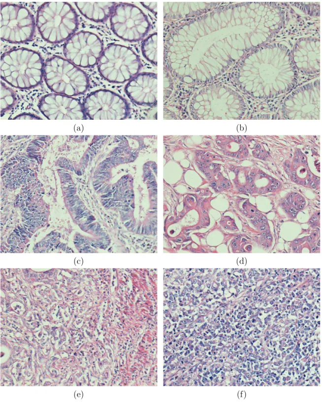
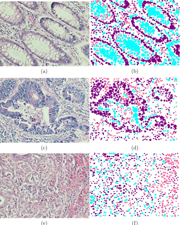
2.2 Examples of colon tissue images: (a)-(b) normal tissues, (c)-(d) low-grade cancerous tissues, and (e)-(f) high-grade cancerous tissues. 8
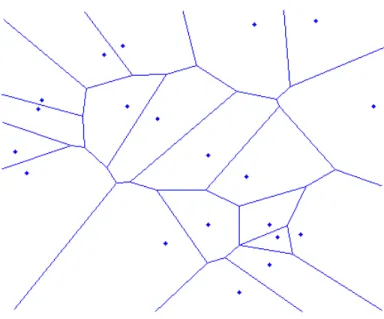
2.3 The Voronoi diagram for randomly selected 20 points . . . 15
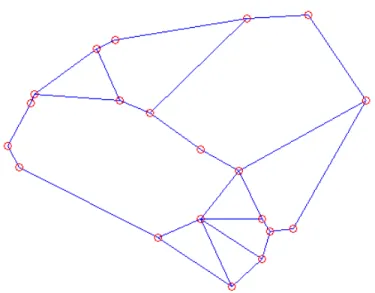
2.4 The Delaunay triangulation for the 20 random selected points . . 16
2.5 The Gabriel’s graph for the same randomly selected 20 points . . 16
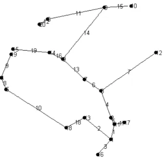
2.6 Minimum spanning tree constructed for the same randomly se-lected 20 points . . . 17
3.1 Examples of tissue images and their located objects. In these im-ages, (a) a normal tissue image, (c) a low-grade cancerous tissue image, (e) a high-grade cancerous tissue image and (b)(d)(f) the objects located on these tissue images. Here purple, pink, and white objects are represented with purple, pink, and cyan, respec-tively. . . 19
LIST OF FIGURES xi
3.2 Extracting local object patterns for the objects shown in black. Here m is selected as 4, thus S =
m
[
j=0
2j-LOP. Sixteen-nearest neighbors of the selected objects are indicated on the examples with their orders. . . 22
4.1 Test set accuracy as a function of the minimum circle radius rmin 37
4.2 Test set accuracy as a function of the highest degree m . . . 38
4.3 Test set accuracy as a function of the cluster number k . . . 39
4.4 Test set accuracy as a function of the subset number N . . . 40
List of Tables
2.1 The most commonly used intensity histogram features . . . 9
2.2 Cooccurrence matrix features . . . 11
2.3 The mostly used run-length matrix features . . . 12
4.1 For textural approaches, considered parameter values are listed. The parameter values selected by three fold cross-validation are indicated as bold. . . 31
4.2 For structural approaches, considered parameter values are listed. The parameter values selected by three fold cross-validation are indicated as bold. . . 31
4.3 Test set results obtained by our proposed algorithms Simple ap-proach and GraphWalk Apap-proach and the textural comparison al-gorithms . . . 34
4.4 Test set results obtained by our proposed algorithms Simple ap-proach and GraphWalk apap-proach and the structural comparison algorithms . . . 35
4.5 For the test set, the confusion matrix obtained by our Simple ap-proach . . . 35
LIST OF TABLES xiii
4.6 For the test set, the confusion matrix obtained by our GraphWalk approach . . . 36
Chapter 1
Introduction
Cancer is one of the most lethal diseases especially in developed and develop-ing countries. Although many tests are present for cancer screendevelop-ing, the routine practice for cancer diagnosis and grading is the histopathological examination of a biopsy, which includes examining biopsy tissues under a microscope and diagnosing cancer based on abnormal tissue formations. Although this exami-nation is the gold standard in the current practice of medicine, it is subject to observer variability since it mainly relies on the visual interpretation of pathol-ogists that heavily depends on their experience and expertise. To alleviate the observer variability, it has been proposed to use computational methods that ex-tract mathematical features to represent histopathological tissue images and use these features for their classification.
The previously proposed automated cancer diagnosis systems typically use one of the following two approaches to define their descriptors: textural and structural. In the literature, there exist several studies that use different texture descriptors for automated cancer diagnosis and grading. The most commonly used descriptors are those that are defined on intensity/color histograms, which quantify the first order statistics of image pixels [1, 2, 3, 4], and cooccurrence matrices, which quantify the second order statistics among pixels [4, 5, 6, 7, 8]. In addition to these, many studies make use of wavelets to define their features.
Examples include the descriptors defined on multiwavelet coefficients [9] and Ga-bor filter responses [10]. Fractal analysis is another method used for defining texture descriptors. In this analysis, fractal dimensions are frequently used as features [1, 11, 12, 13]. More recent studies use local binary patterns to define additional texture descriptors [14, 15, 16, 17, 18]. They are used to quantify a pixel according to spatial arrangement of its neighbors’ intensities with respect to its intensity. All these texture descriptors yield promising results. However, they are defined on pixels, directly using pixels’ intensity/color values. Thus, they are susceptible to pixel-level noise and variations that are typically observed in histopathological images.
To alleviate the negative aspects of pixel-level noise and variations, structural approaches have been proposed. These approaches are defined to model the spa-tial relationships of histological components to represent a tissue image. These approaches commonly construct a graph on these components and use graph de-scriptors for image classification. Earlier studies construct their graphs on only nucleus tissue components using different techniques such as Delaunay triangu-lations [7, 10, 19, 20, 21]. minimum spanning trees [19, 22, 21], and probabilistic graph generations [23]. In the recent study of our research group [24], we con-struct a graph on tissue components of different types and color graph edges based on the types of their end nodes. Different than the descriptors proposed in this thesis, these previous structural approaches usually use a global graph representation for the entire image and extract global graph descriptors for its quantification.
1.1
Contribution
In this thesis, we propose a new algorithm for effective and robust representa-tion and classificarepresenta-tion of images of histopathological colon tissues stained with hematoxylin-and-eosin. In the proposed algorithm, our main contributions are the introduction of a set of new texture descriptors, which we call local object patterns, to model composition of histological components in a tissue image and
the use of this descriptor set to define the visual words of the bag-of-words rep-resentation of the image. To this end, we decompose the image into component objects of multiple types and define texture of these objects using the idea of local binary patterns [25]. However, as opposed to local binary patterns defined at the pixel-level, we define local object patterns on the objects at the component-level. Particularly, local binary patterns are defined to quantify a pixel by constructing a binary string from the spatial arrangement of its neighbors’ relative intensities. On the other hand, we define our local object patterns to quantify an object by specifying a set of neighborhoods with different locality ranges and constructing a string based on how the object’s neighbors arrange in an order in each of these local neighborhoods. Our texture definition proposed in this thesis mainly differs from the previous texture-based tissue classification studies in the following as-pect: It defines its texture descriptors on higher-level component objects instead of defining them at the pixel-level.
In the proposed algorithm, the defined local object patterns are used to char-acterize the tissue objects, the type distribution of which is used to construct bag-of-words representations of the tissue. In this thesis, we implement two al-gorithms for this construction. The first approach (Simple approach) uses the type distribution of the objects to construct a single bag-of-words representation. The second one (GraphWalk approach) uses the type distributions of the object subsets obtained through graph walking to construct multiple bag-of-words repre-sentations and combines them by voting. Different than the previous approaches, this thesis uses the object distributions whose types are assigned by making use of their local object patterns. Moreover, the use of graph walks to obtain multiple object subsets is another contribution of this thesis.
The algorithms proposed by this thesis are tested on 3236 microscopic colon tissue images. The experiments reveal that our proposed texture descriptors are effective to obtain better classification accuracies compared to previous texture definitions.
1.2
Outline of the Thesis
This thesis is structured as follows. In Chapter 2, we give details of the back-ground information about the problem domain and summarize the previous com-putational methods used for automated cancer diagnosis and grading. In Chapter 3, we present our proposed local object pattern algorithm, providing the details of decomposing an image into components, defining local object patterns on these components, and using these patterns for image classification. In Chapter 4, we explain the dataset, and discuss the experimental results. Finally, in Chapter 5, we provide the summary of the thesis and discuss its future research directions.
Chapter 2
Background
In this chapter, we briefly give domain description of colon tissues and colon cancer. Then, we present the approaches that are used in the literature for automated cancer diagnosis.
2.1
Domain Description
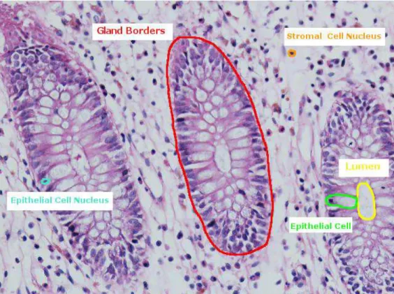
This thesis focuses on representation of colon tissues and classification of colon adenocarcinoma. Colon tissues contain hierarchical structures called glands. These glands are formed of epithelial cells lined up around a lumen, which is an inner open space of a tubular structure and absorbs water and minerals while secreting mucus. Besides these gland structures, colon tissues contain stroma, which is a connective tissue and contains non-epithelial cells. These basic parts of a colon tissue are shown on an example image in Figure 2.1.
Colon cancer is one of the four major cancer sites [26], which results in un-controlled cell growth in colon tissues. Colon adenocarcinoma is the cancer type that accounts for 90-95 percent of all colorectal cancers. Colon adenocarcinoma originates from epithelial cells forming the glandular structures in colon tissues. Thus, it causes changes in the glandular structures. Figure 2.2 shows normal
Figure 2.1: An image of a normal colon tissue stained with hematoxylin and eosin, which is the routinely used technique to stain biopsies in hospitals.
and adenocarcinomatous colon tissues. As shown in this figure, gland structures deform with the existence of cancer. This deformation is less and the glands are still differentiated in low-grade cancerous tissues whereas the deformation increases and the glands are only poorly differentiated in high-grade cancerous tissues. In this thesis, we focus on classifying tissue images into three classes: normal, low-grade cancerous, and high-grade cancerous.
The final diagnosis of colon adenocarcinoma is done via histopathological ex-amination of colon biopsies. In this process, a small amount of sample tissue (biopsy) is taken from the body with a special instrument and then is fixed, cut into thin pieces, and stained for microscopic examination. The staining technique that is mostly used in hospitals is called hematoxylin-and-eosin (H&E). In this staining, hematoxylin stains cell nuclei blue-purple and eosin stains proteins and other cellular elements in a tissue pink-red; background remains colorless [27]. The example tissue images obtained with this staining are shown in Figure 2.1 and Figure 2.2.
2.2
Automated Cancer Classification
In this section, we will explain the previous methods that are used for automated diagnosis and grading of cancer. These methods can be mainly grouped into two: textural and structural. We will explain these methods in the following subsections.
2.2.1
Textural Methods
Textural methods are essential in the image analysis based on local spatial varia-tions of intensity or color. These methods aim to draw conclusion for an unknown image by using a known texture. Textures are obtained from images using various texture feature extraction methods such as cooccurrence matrix features, fractal dimensions, run-length features, wavelet features, and entropy [28].
(a) (b)
(c) (d)
(e) (f)
Figure 2.2: Examples of colon tissue images: (a)-(b) normal tissues, (c)-(d) low-grade cancerous tissues, and (e)-(f) high-low-grade cancerous tissues.
2.2.1.1 Color and Intensity Histogram Features
Histograms characterize an image according to its color distribution or intensity. The color histogram is used for cancer diagnosis [1, 2, 3]. It uses joint probabilities of intensities in the red, green, and blue color channels. It divides the image into bins and stores the pixels of each color channels. It can be formalized as
hR,G,B(a, b, c) = N · P rob (R = a, G = b, B = c) (2.1)
where R, G, and B are the three color channels and N is the number of pixels in the image.
Intensity histogram illustrates the frequency of pixels in a grayscale image with L levels of intensity found in the image. It is a discrete function h(rk) = nk
where rk is the kth gray level and nk is the frequency of pixels in the gray level rk
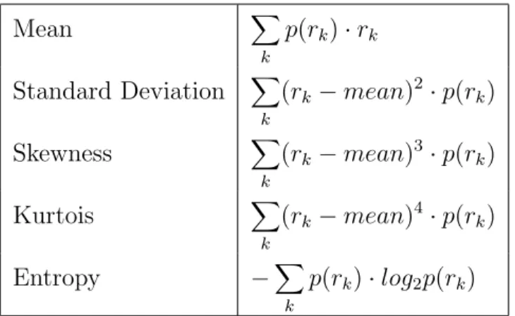
in range [0 - L]. The mean, standard deviation, skewness, kurtosis, and entropy (Table 2.1) are extracted from the histogram probability density function [4]. p(rk) =
h(rk)
M where M is the number of pixels, and p(rk) should satisfy the following properties. p(rk) >= 0 L X g=0 p(g) = 1
Table 2.1: The most commonly used intensity histogram features
Mean X k p(rk) · rk Standard Deviation X k (rk− mean)2· p(rk) Skewness X k (rk− mean)3· p(rk) Kurtois X k (rk− mean)4· p(rk) Entropy −X k p(rk) · log2p(rk)
2.2.1.2 Cooccurrence Matrix Features
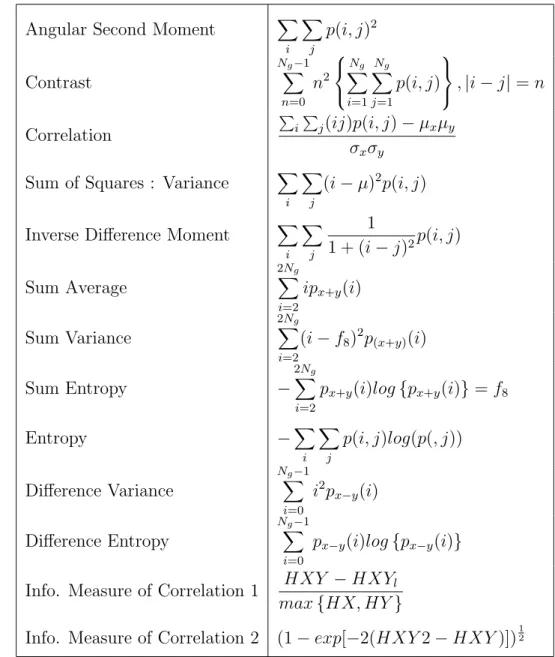
The most widely used features for textural analysis are Haralick features ex-tracted from cooccurrence matrices [29]. They are calculated to quantify the relationship among two pixels that cooccur at a specific distance and direction. For a given direction Q and distance d, cooccurrence matrix keeps the frequency of occurrences of gray levels i and j. The features extracted from a coccurrence matrix are summarized in Table 2.2 where p(i,j) is the frequency of cooccurrence of gray levels i and j, µ is the mean, and σ is the standard deviation. Although, 14 texture features are initially proposed, only four of them, which are angular second moment, contrast, correlation, and entropy are widely used. A cooccur-rence matrix is a second order statistics that defines how often different variation of pixel gray levels cooccur in an image. Cooccurrence matrix denotes various characteristic of the spatial distribution of the gray levels in entire images so the features are used in tissue analysis [4, 6, 7, 8].
2.2.1.3 Run-Length Matrix Features
In cancer diagnosis and grading, higher order statistics [30] extracted from run-length matrices are also used [31, 32, 33]. Run-run-length is modeled as a pattern of the length of the scanned line of each image in pixels. A primitive is defined as a continuous set of maximum number of pixels both in the same gray levels and in the same direction [34]. A number of primitives of all directions p(a,r), (where length r with a gray level in an M x N image) is used for extracting the features. Galloway [30] extracts five features whereas Chu [35] defines two more new features. Finally, Dasarathy and Holder [36] extend the features by defining new four features. Table 2.3 illustrates the mostly used run-length matrix features for cancer diagnosis and grading. In this table, K =
L X a=1 Nr X r=1
is the total number of runs, L is the number of gray levels, and Nr is the the maximum length.
Table 2.2: Cooccurrence matrix features
Angular Second Moment X
i X j p(i, j)2 Contrast Ng−1 X n=0 n2 Ng X i=1 Ng X j=1 p(i, j) , |i − j| = n Correlation P i P j(ij)p(i, j) − µxµy σxσy
Sum of Squares : Variance X
i
X
j
(i − µ)2p(i, j)
Inverse Difference Moment X
i X j 1 1 + (i − j)2p(i, j) Sum Average 2Ng X i=2 ipx+y(i) Sum Variance 2Ng X i=2 (i − f8)2p(x+y)(i) Sum Entropy − 2Ng X i=2
px+y(i)log {px+y(i)} = f8
Entropy −X i X j p(i, j)log(p(, j)) Difference Variance Ng−1 X i=0 i2px−y(i) Difference Entropy Ng−1 X i=0
px−y(i)log {px−y(i)}
Info. Measure of Correlation 1 HXY − HXYl max {HX, HY }
Table 2.3: The mostly used run-length matrix features
Short primitive emphasis 1 K L X a=1 Nr X r=1 p(a, r) r2
Long primitive emphasis 1 K L X a=1 Nr X r=1 p(a, r)r2
Gray level uniformity 1 K L X a=1 [ Nr X r=1 p(a, r)r2]2
Primitive length uniformity 1 K L X a=1 [ Nr X r=1 p(a, r)]2 Primitive percentage PL K a=1 PNr r=1p(a, r) = K M N
2.2.1.4 Law’s Texture Energy Measures
It has been proposed to use Laws’ texture energy measures [37] to describe tex-tures for cancer diagnosis and grading [38]. The Laws’ texture featex-tures are similar to the Haralick’s [29] co-occurrence matrix features [29]. They calculate texture energies in the spatial domain. Given one-dimensional kernels merged into con-volution masks, which output the energy image and every pixel located at the center of the local window’s l(i,j) are replaced with the absolute value in the filter window f(i,j) where n is the size of the mask as given below:
s(i, j) = 1 (2xn + 1)2 i+n X k=i−n j+n X l=j−n |f (k, l) − l(i, j)| (2.2) 2.2.1.5 Fractal Analysis
Fractal geometry is used for cancer diagnosis and grading [1, 12, 13]. The fractal dimension is the most commonly used feature in fractal analysis and computes the self-similarity property. Although there exist various fractal dimension algo-rithms, the box-counting method [39] is commonly used due to its cost efficiency, high accuracy, and implementation ease [13]. The formula for the box-counting method is given in Equation 2.3.
DB = −lim
logN∈(S)
log(∈) (2.3)
2.2.1.6 Multiwavelet Features
Wavelets create whole representation of signals by using all of the sub-band de-composition and allow the image dede-composition into various frequency sub-bands. Wavelets utilize one scaling function, whereas multiwavelets use more than one scaling function. In cancer diagnosis and grading, wavelets are employed to ex-tract features from the wavelet coefficients (like entropy and energy) [9] and from Gabor filter responses [7].
2.2.1.7 Local Binary Patterns
Local binary patterns define the relationship between a pixel and its neighborhood pixels. Initially, Ojala et al. [40] proposed a method where neighbor pixels whose intensities are higher than or equal to the value of the center pixel are labeled with 1 and the others are labeled with 0. The method is improved by considering the neighbors which are radius r distance far away from the center pixel [25]. The neighbors are counted clockwise to get the binary value as follows:
LBPp,r= p−1 X n=0 s(xr,n− x0,0)2n, 1, x ≥ 0 0, x < 0 = s(x)
where x0,0 is center pixel and p is the number of neighbor pixels around radius
circle r.
In cancer diagnosis, local binary pattern texture features are usually combined with other features by various methods [14, 15, 16, 17, 18].
2.2.2
Structural Methods
Textural approaches may suffer from noise and variation commonly observed at the pixel-level of tissue images. On the other hand, structural approach define their features at the component level to mitigate the pixel-level problems. In au-tomated cancer diagnosis, graph based methods are widely used as structural ap-proaches. In these methods, nodes are mostly the nuclear components and edges are defined for encoding the spatial information among the nodes. Voronoi dia-grams, Delaunay triangulations, minimum spanning trees, probabilistic graphs, weighted graphs, and color graphs are the most common graph generation algo-rithms. These generation methods will be discussed in the following subsections.
2.2.2.1 Voronoi Diagrams
The Voronoi diagram of a point set S divides the n points in the set S into n regions where p ∈ S contains all points in the plane such that p is the nearest site [41]. Figure 2.3 illustrates the Voronoi diagram of randomly selected 20 points. The features extracted from a Voronoi diagram include the area, roundness, aspect ratio, circularity, and the number of sides. They are commonly used with the features extracted from Delaunay triangulation [7, 19, 20, 21].
2.2.2.2 Delaunay Triangulations
A triangulation of S is a planar graph with a vertex set where all the bounded faces are triangles and S is a set of n points. The Delaunay triangulation of S is a dual graph of the Voronoi diagram where the edges are straight lines and each vertex is located in the set S. Delaunay triangulation are used in many cancer diagnosis and grading algorithms [19, 42, 43]. Triangulations are characterized by using structural features such as the area, edge length, degree of nodes, distance to the nearest neighbor, eccentricity, clustering coefficient, shortest paths between nodes, and diameter. Figure 2.4 shows the Delaunay triangulation of the same randomly selected 20 points used in the construction of the Voronoi graph given
Figure 2.3: The Voronoi diagram for randomly selected 20 points
in Figure 2.3. Note that it is also possible to use Gabriel’s graph to extract such features [44]. Such as a Gabriel graph is shown in Figure 2.5.
2.2.2.3 Minimum Spanning Trees
In graph theory, a spanning tree T, is a sub-graph of a connected, undirected graph G = (W, E) that includes every vertex of the graph G. A minimum span-ning tree of graph G is the spanspan-ning tree, for which the sum of edge weights is minimized. Like Voronoi diagrams and Delaunay triangulations, structural fea-tures are extracted from minimum spanning trees. These are the edge length, degree of nodes, distance to the nearest neighbor, fractal dimension, eccentric-ity, clustering coefficient, and diameter [19, 21, 22]. Figure 2.6 demonstrates the minimum spanning tree of the same randomly selected 20 points.
Figure 2.4: The Delaunay triangulation for the 20 random selected points
Figure 2.6: Minimum spanning tree constructed for the same randomly selected 20 points
2.2.2.4 Color Graphs
Structural approaches explained above characterize the spatial distribution of cell nuclei. However, color graphs model the spatial distribution of the nucleus, stroma, and luminal structures [24]. In this graph, these tissue components are represented as nodes and their relations are encoded constructing a graph on these nodes. Graph edges are then colored according to the component types of the edges’ endpoints. Features extracted from the color graphs are the colored average degree, colored average clustering coefficient, and colored diameter.
Chapter 3
Methodology
Our proposed algorithm introduces a new texture descriptor, which we call local object patterns, to model tissue images and uses these descriptors for tissue image classification. To this end, it decomposes a tissue image into its histological components, characterizes them with the newly introduced local object pattern descriptors, and uses this characterization for classification of tissue images. In the following sections, the details of the proposed algorithm are provided.
3.1
Tissue Image Decomposition
We model a tissue image I by approximately representing its histological com-ponents with a set of circular objects O(I) = {oi}. We represent each object oi
by its coordinates (xi, yi) and its type ti ∈ {purple, pink, white} . These types
correspond to the three main colors in a hematoxylin-and-eosin stained tissue. Particularly, cell nuclei correspond to purple; stroma, stromal cells’ cytoplasms, and mucin-poor epithelial cells’ cytoplasms correspond to pink; and lumina and mucin-rich epithelial cells’ cytoplasms correspond to white. Since there are mul-tiple components corresponding to the same type, we hereinafter refer them to as purple, pink, and white, to keep the thesis simpler and easier to read.
(a) (b)
(c) (d)
(e) (f)
Figure 3.1: Examples of tissue images and their located objects. In these images, (a) a normal tissue image, (c) a low-grade cancerous tissue image, (e) a high-grade cancerous tissue image and (b)(d)(f) the objects located on these tissue images. Here purple, pink, and white objects are represented with purple, pink, and cyan, respectively.
In order to define the circular object set O(I) = {oi}, we first separate
hema-toxylin and eosin channels of the image I by applying a color deconvolution method [45]. Then, we quantize pixels into three groups (pink, white, and purple which are the main colors in the hematoxylin and eosin stained tissues) according to the color convolution. Particularly, we assign pixel pi into one of these groups
as follows: pi = purple if hi ≤ havg
pink else if ei ≤ eavg
white otherwise
where hi and ei are the hematoxylin and eosin component values of the pixel pi
and havg and eavg are the average values of the hematoxylin-and-eosin component
values over all pixels. After pixels are labeled, we apply the circle fit algorithm [46] to each group’s pixels to locate the objects. In this algorithm, the objects are located if radii are greater than the threshold radius rmin. Figure 3.1 illustrates
the objects located on example tissue images.
In our model, we use an approximate representation instead of finding exact locations of histological components because their exact localization gives rise to a quite difficult segmentation problem. Thus, there may be one-to-one or many-to-one relation between objects and components. For example, a purple object usually corresponds to a single nucleus, whereas a group of white objects that form a clique corresponds to a lumen region. The proposed local binary patterns are also effective to model such many-to-one relations.
3.2
Local Object Patterns
For object oi, the nth local object pattern n-LOP(oi) is defined as follows: we first
find the distance from the coordinate (xi, yi) of oi to the coordinate of every other
object in the object set O = {o1, ..., oi, ..., ok} and select the n nearest neighbors
of oi to get the ordered neighbor set N (oi) = {oin, ..., oij, ..., oi1}. After that, we
bij = 1 if tij ∈ {purple} 0 if tij ∈ {pink, white}
where tij is the type of the selected neighbor oij. Then, we define 2j-LOP(oi)
as the decimal equivalent of the binary string B(oi). Note that this descriptor
provides rotation invariance since objects are ordered based on their distances to object oi and its value does not change with arbitrary rotations of the image.
We define local object patterns for an object to quantify the spatial arrange-ment of its neighbors’ types found in a local neighborhood. In our model, we extract a set of (m + 1) patterns using different neighborhoods. Particularly, this set includes S =
m
[
j=0
2j-LOP.
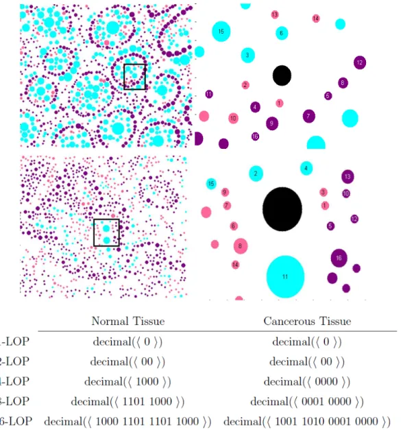
Figure 3.2 illustrates extraction of local object patterns for the objects shown in black. We select these objects such that they both belong to luminal regions; we crop these regions from normal and cancerous tissue images as shown in Fig-ure 3.2. This illustration shows that although lower-order patterns are the same for the two selected objects, their higher-order patterns show differences, which can be used to differentiate these objects.
By using the local object pattern descriptors, we define the new object types as follows: For each original type ti ∈ {purple, pink, white}, we
sepa-rately cluster objects of the corresponding type into k groups running the k-means algorithm on local object patterns of these objects. Thus, we learn k clustering vectors Vpurple = {v1, v2, ..., vk} for the purple type, k
cluster-ing vectors Upink = {u1, u2, ..., uk} for the pink type, and k clustering vectors
Wwhite = {w1, w2, ..., wk} for the white type. Then, for a given image, we relabel
each object oi with a new type t
0
i based on its original type ti and the
corre-sponding set of the clustering vectors Vpurple, Upink or Wwhite. Since components
(objects) of normal and cancerous tissue images show different neighbor distribu-tions, they are expected to be relabeled with different types t0i. Thus, we use the distribution of these new types to represent an image. In our work, we use the distribution of the new types in two different ways. We will explain these ways
Figure 3.2: Extracting local object patterns for the objects shown in black. Here m is selected as 4, thus S =
m
[
j=0
2j-LOP. Sixteen-nearest neighbors of the selected objects are indicated on the examples with their orders.
in the following section.
3.3
Tissue Classification
After characterizing the objects of an image I, we use this characterization to represent the image. For that, we use the bag-of-words representation on the frequency of objects’ new types. Here we use two approaches to obtain the bag-of-words representation.
In the Simple Approach, we use the new types of all objects in the image to extract the bag-of-words representation and classify the image using a linear kernel support vector machine (SVM) classifier.In our work, we use the SVM library given in [47]. Here since our problem involves more than two classes, this implementation uses one-against-one strategy for this multiclass classification. This strategy constructs k(k − 1)/2 classifiers, each of which differentiates one class from another. Then the decisions of these classifiers are voted to obtain the final class.
In the GraphWalk Approach, we obtain multiple subsets of the objects and separately use the frequency of their types to obtain multiple bag-of-words repre-sentations of the same image. Here we use this approach to explore the following: when all objects are used to create a bag-of-words representation, this gives a global feature set of the entire image. However, in tissue images, there may exist some local subregions that may be more important than the others. By selecting object subsets that correspond to such local regions, we aim to extract feature sets corresponding to these potentially important subregions.
In this second approach, we first construct a graph on the entire objects by using Delaunay triangulation and then employ the breadth first search (BFS) algorithm to select an object subset. We finally use the frequency of the new types of these selected objects to construct a bag-of-words representation. Particularly, the BFS algorithm traverses graph nodes, which correspond to the objects, level-by-level starting from an initial node (object). In our algorithm, we start the
BFS algorithm from each of the N largest white objects and obtain an object subset. Here we terminate the BFS algorithm, after it traverses L objects in the graph. Here it is worth to noting that the number L of visited objects is less than the number of the entire objects in the image. Thus, the selected object subsets are expected to cover a smaller local region in the tissue image. In our work, we classify each of these bag-of-words representations with linear kernel SVMs and combine the decisions of these SVMs through simple voting.
Chapter 4
Experimental Results
In this chapter, we first give the details of our dataset. Then, we explain the methods that we use in our comparisons. Later, we explicate the parameters of our algorithms. After that, we give our results and compare them with the comparison methods to understand how efficient and accurate our proposed algo-rithms are. Finally, we provide the effects of the selection of the model parameters to classification accuracy.
4.1
Dataset
Our dataset contains 3236 microscopic images of colon tissues stained with hematoxylin-and-eosin. The images are taken from the 258 randomly selected patients from the Pathology Department in Hacettepe University School of Medicine. They are acquired by a Nikon Coolscope Digital Microscope using 20× microscope objective lens and 480 × 640 image resolution.
Images are randomly divided into two groups as training and test sets. The 1644 images of randomly selected patients constitute the training set and 1592 images of the rest of the patients constitute the test set. Each image in these sets is labeled as normal, low-grade cancerous, or high-grade cancerous. The
training set contains 510 normal, 859 low-grade cancerous, and 275 high-grade cancerous tissues of 129 patients. The test set contains 491 normal, 844 low-grade cancerous, and 257 high-grade cancerous tissues of the remaining 129 patients.
4.2
Comparisons
We use two groups of approaches in our comparison: textural and structural. These comparison approaches are given in the following subsections.
4.2.1
Textural Approaches
First, we compare our algorithm that defines texture descriptors at the component level with the textural approaches that define their descriptors at the pixel level. These are intensity histograms, gray-level cooccurrence matrices, and local binary patterns. These approaches use linear kernel SVMs in their classification.
4.2.1.1 Intensity Histogram Approach
First order histogram features are derived from the gray-level intensities of image pixels. They include mean, standard deviation, kurtosis, and skewness. To reduce noise and small intensity variations, pixel intensities are grouped into N bins [4].
We also implement the grid based variant of the Intensity Histogram approach. Here we decide to use a grid-based variant since it is commonly difficult to find a constant texture over an entire image as the tissue image may contain sub-regions irrelevant to classification. In this approach, we divide the image into fix-size grids, extract a histogram on each grid, calculate descriptors on the grid histograms, and average these descriptors all over the image.
4.2.1.2 Cooccurrence Matrix Approach
Second order statistics are calculated on the gray level intensities of image pixels. In our comparisons, we use textural features that are extracted from cooccurrence matrices at eight orientations. These features include the angular moment to model homogeneity of a tissue image, the entropy to model randomness, the contrast and difference moment to model local variations, the correlation function to model linearity of gray-level dependencies, the inverse difference moment to model local homogeneity, the dissimilarity to measure the dissimilarity between pixels [5].
Likewise, we also use a grid-based variant of the Cooccurrence Matrix ap-proach. Similarly, we divide the image into fixed size grids, extract cooccurrence matrix features from each of these grids and average them all over the grids [48].
4.2.1.3 Local Binary Pattern Approach
The Local Binary Pattern descriptors include histogram frequencies. We compute this histogram on the outputs of a uniform local binary pattern (LBP) operator applied on image pixels. For each pixel, the LBP operator [25] outputs a binary string by comparing the pixel’s gray-scale intensity with those of its eight neigh-bors; it outputs 1 if its intensity is lower and 0 otherwise. It then assigns the pixel to a histogram bin based on the number of consecutive 1’s in this binary string. This operator is called uniform if it constructs the histogram on only the pixels whose binary strings contain at most two bitwise 0/1 transitions in their circular chain. We calculate an additional bin for keeping frequencies of pixels with non-uniform strings. In our experiments, we extract these descriptors from the histogram constructed on all pixels. Here we did not implement its grid based variant because calculating histograms on pixels of equal-sized grids and averaging their histogram frequencies is equivalent to calculating a histogram on all pixels and using its frequencies.
4.2.1.4 Pixel Based Approach
This is the pixel-based counterpart of our algorithm. This approach follows ex-actly the same steps of our algorithm except its descriptor definition step. Partic-ularly, it decomposes a tissue image into a set of circular objects, defines descrip-tors on the objects, clusters the objects based on their descripdescrip-tors to find their new types, and uses the new types’ frequency in a linear kernel SVM classifier. Here different than our proposed algorithm, which uses local object patterns as the descriptors, the Pixel Based approach uses local binary patterns. To this end, it locates a square window at the center of each object and calculates local binary patterns of this window to find the descriptors of the object. We use this comparison in our experiments to understand the effectiveness of defining component-level local object patterns.
4.2.1.5 Resampling-based Markovian Model
Additionally, we use the Resampling-based Markovian Model (RMM) that we previously implemented in our research group [48]. The RMM obtains multiple samples of an image, labels each sample using discrete Markov models, and votes the samples’ labels to classify the image. To obtain an image sample, it gen-erates a sequence on the randomly selected points, which are characterized by texture descriptors and ordered based on proximity. These descriptors include the histogram of quantized pixels and the J-value texture measure.
4.2.2
Structural Methods
Next, we compare our algorithm with previous structural approaches. These approaches construct graphs on tissue components and extract features on these constructed graphs. Likewise, these approaches use linear kernel SVM classifiers. The details of these methods are given below:
4.2.2.1 Delaunay Triangulation
This approach defines its graph constructing Delaunay triangulation on nuclear (purple) objects located by the circle fit algorithm. Then it extracts global fea-tures from this Delaunay triangulation. These feafea-tures include the average, stan-dard deviation, minimum-to-maximum ratio, and disorder of edge lengths and triangle areas, as well as the average degree, average clustering coefficient, and diameter of the entire Delaunay graph [10].
4.2.2.2 Color Graph
This is similar to the Delaunay Triangulation approach except that it constructs its graph on all types of tissue components. Particularly, it constructs Delaunay triangulation on all objects but colors the triangle edges based on the types of the end nodes. Then, it extracts colored version of the global features including the average degree, average clustering coefficient, and diameter [24].
4.2.2.3 Hybrid Model
The last method is the Hybrid Model that we recently developed in our research group [49]. This model first represents an image with an attributed graph and defines smaller query graphs as a reference to normal gland structures. It then selects regions of the image whose subgraphs are most structurally similar to the query graphs based on graph edit distances. Using the graph edit distances of the selected regions as well as their texture descriptors, it classifies the image by a linear kernel SVM.
4.3
Parameter Selection
We used two algorithms to define bag-of-words representations: Simple approach, which employs all objects, and GraphWalk approach, which uses object sets ob-tained by graph walking. The parameters of these algorithms are explained in the following subsections. We also explain the parameters of the comparison algorithms.
In all algorithms, we use three fold cross validation on the training set for parameter selection. In order to do that, we list all possible values of each pa-rameter and then test all possible papa-rameter combinations in the list, and select the one that yields the highest cross-validation accuracy. The three fold cross validation method divides the training set into three equal parts. It trains the set with the two subsets and tests the classifier with the third one. It repeats this for three times in each of which the classifier is tested with a different subset. Note that we consider the highest average accuracy obtained on the test subsets.
4.3.1
Simple Approach
The Simple approach has three model parameters:
Minimum Radius rmin
The minimum circle radius of the objects in tissue images Highest Degree m
The highest degree in determining how many nearest neighbors should be selected
Cluster Number k
The cluster number for grouping the objects of each original type in tissue images
In addition to these parameters, we have an additional parameter C for the SVM classifier with a linear kernel [47]. In our experiments, we used all possible
Table 4.1: For textural approaches, considered parameter values are listed. The parameter values selected by three fold cross-validation are indicated as bold.
Intensity Histogram C ∈ {1, 2, ..., 9, 10, 20, ..., 90, 100, 150, 200, ..., 1000} Bin numbers ∈ {4, 8, 16, 32}
Intensity Histogram Grid
C ∈ {1, 2, ..., 9, 10, 20, ..., 90, 100, 150, .., 550, ..., 1000} Bin numbers ∈ {4, 8, 16, 32} Grid Size ∈ {10, 20, 40, 80} Cooccurrence Matrix C ∈ {1, 2, ..., 9, 10, 20, ..., 90, 100, 150, ..., 900, 1000} Bin numbers ∈ {4, 8, 16, 32} Distance ∈ {5, 10, 20, 40}
Cooccurrence Matrix Grid
C ∈ {1, 2, ..., 9, 10, 20, 30, ..., 90, 100, 150, ..., 1000} Bin numbers ∈ {4, 8, 16, 32}
Distance ∈ {5, 10, 20, 40} Grid Size ∈ {10, 20, 40, 80}
Local Binary Pattern C ∈ {1, 2, ..., 9, 10, 20, ..., 90, 100, 150, 200, ..., 700, .., 1000}
RMM C ∈ {1, 2, 3..., 9, 10, 20, ..., 90, 100, 150, ..., 1000} winSize ∈ {10, 20, 40, 80} StateNo ∈ {4, 8, 16, 32, 64} SeqLen ∈ {10, 25, 50, 100, 150} SeqNo ∈ {10, 25, 50, 100, 150}
Pixel Based Approach
C ∈ {1, 2, ..., 9, 10, 20, ..., 60, .., 100, 150, 200, .., 1000} rmin ∈ {3, 4, 5}
k ∈ {5, 10, 20, 30}
winSize ∈ {10, 20, 40, 80}
Table 4.2: For structural approaches, considered parameter values are listed. The parameter values selected by three fold cross-validation are indicated as bold.
Delaunay Triangulation
C ∈ {1, 2, ..., 9, 10, 20, ..., 90, 100, 150, ..., 900, 1000} Structing element size ∈ {3, 5, 7, 9}
Circle area threshold ∈ {5, 10, ..50}
Color Graph
C ∈ {1, 2, 3..., 9, 10, 20, ..., 90, 100, 150, ..., 1000} Structing element size ∈ {3, 5, 7, 9}
Circle area threshold ∈ {5, 10, ..50}
Hybrid Model
C ∈ {1, 2, 3..., 9, 10, 20, ..., 90, 100, 150, ..., 1000} W ∈ {10, 20, 40, 60, 80}
combinations of the following parameter sets rmin ∈ {3, 4, 5} , m ∈ {2, 3, 4, 5} ,
k ∈ {5, 10, 20, 30} and C ∈ {1, 2, .., 9, 10, 20, ..., 90, 100, 150, ..., 950, 1000}. In our experiments, we get the highest cross-validation accuracy for rmin = 4, m = 4, k
= 20, and C = 20.
4.3.2
GraphWalk Approach
The GraphWalk approach has the following parameters:
Subset Number N
The number of object subsets selected by the breadth first search algorithm Visited Object Number L
The number of visited objects during the breadth first search algorithm
Highest Degree m
The highest degree in determining how many nearest neighbors should be selected
Cluster Number k
The cluster number for grouping the objects of each original type in tissue images
This approach has also the parameter C for the SVM classifier [47]. In its parameter selection, we use the following combinations of the parameter sets m ∈ {2, 3, 4, 5}, k ∈ {60, 70, 120, 150}, N ∈ {25, 50, 75, 100}, L ∈ {25, 50, 75, 100}, and C ∈ {1, 2, ..., 9, 10, 20, ..., 90, 100, 150, ...400, ..., 1000}. We obtain the highest cross validation accuracy for m = 4, k = 70, N = 25, L = 100 and C = 400.
4.3.3
Comparison Algorithms
We also use three fold cross-validation on the training set to select the parameters of the comparison algorithms. The lists of the considered parameter values for
textural and structural approaches are given in Table 4.1 and Table 4.2, respec-tively. The selected parameters of each approach are shown as bold.
4.4
Results
We implement local object patterns to represent and classify tissue images. We characterize the objects using these local object patterns and construct bag-of-words representation using two approaches: Simple approach and GraphWalk approach. In order to understand the efficiency of these algorithms, we compare them with the previous textural and structural algorithms. The test results are given in the Table 4.3 and Table 4.4 for textural and for structural algorithms, respectively. These tables show that our proposed algorithms give high accuracies for all classes.
Our algorithm has a similar methodology to the Pixel Based approach and differentiate only in the definition of its descriptors. The Pixel Based approach uses pixel-based local binary patterns as descriptors whereas our methods use object-based local patterns. When we compare these algorithms, our proposed approaches give higher accuracies in all classes and surpass the Pixel Based ap-proach in grading high-grade cancerous tissues. The results show that defining local object patterns instead of local binary patterns increases the efficiency of tissue image classification.
The Intensity Histogram, Cooccurrence Matrix, and Local Binary Pattern ap-proaches extract global texture descriptors on the entire tissue images and their grid-based variants make use of grids to extract their descriptors. The RMM ap-proach extracts its pixel-based texture descriptors locally defined for the selected points. On the other hand, the proposed algorithm extracts texture descriptors for each object in a local neighborhood defined by the distance from this object to its 2m-nearest neighbor. The results show that using object-based textures is more effective to obtain higher accuracies. The grid based variants improve results; however, they are still lower than the results of the proposed algorithm.
The Delaunay Triangulation and Color Graph approaches also use the circular objects and they construct graphs on these objects and extract global properties from these graphs. The Hybrid Model approach uses local graphs for the selected regions. Our Simple approach gives higher accuracies compared to these struc-tural algorithms whereas our GraphWalk approach gives higher results than the Delaunay Triangulation and Color Graph approaches and similar results with the Hybrid Model approach. However, when we look at the accuracies of separate classes, we observe that the GraphWalk approach gives more balance results for the discrimination of different classes.
Table 4.3: Test set results obtained by our proposed algorithms Simple approach and GraphWalk Approach and the textural comparison algorithms
Normal Low-Grade High-Grade Overall Simple Approach (LOPs) 95.32 92.54 90.27 93.03 GraphWalk Approach (nLOPs) 93.68 91.23 90.66 91.90 Intensity Histogram 80.65 69.55 70.04 73.05 Cooccurrence Matrix 83.10 81.64 77.82 81.47 Local Binary Pattern 92.67 73.46 80.54 80.53 Intensity Histogram Grid 78.82 74.17 78.60 76.32 Cooccurrence Matrix Grid 87.58 84.12 85.60 85.43
RMM 95.64 87.77 88.56 90.32
Pixel Based Approach 94.50 90.17 76.65 89.32
We propose two algorithms for defining bag-of-words representations: Simple approach and GraphWalk approach. The Simple approach defines a bag-of-words representation on the frequency of the types of all objects in the image. On the other hand, the GraphWalk approach obtains multiple subsets of the objects via graph walking and constructs multiple bag-of-words representations from these object subsets. In this thesis, we define the second approach to understand the
Table 4.4: Test set results obtained by our proposed algorithms Simple approach and GraphWalk approach and the structural comparison algorithms
Normal Low-Grade High-Grade Overall Simple Approach (LOPs) 95.32 92.54 90.27 93.03 GraphWalk Approach (nLOPs) 93.68 91.23 90.66 91.90 Delaunay Triangulation 89.61 71.56 87.55 79.71 Color Graph 92.67 82.46 86.38 86.24 Hyrid Model 96.95 88.27 96.11 92.21
Table 4.5: For the test set, the confusion matrix obtained by our Simple approach Computed
Normal Low High
Actual
Normal 468 19 4 Low 16 781 47 High 0 25 232
effects of using the characterizations of local subregions instead of using the en-tire image characterization. Our experiments show that although this second approach gives better results than most of the comparison algorithms, it gives statistically significantly worse results than our Simple Approach (we use Mc-Nemars statistical test with a significance level of 0.05). The confusion matrices for these two algorithms are also given in Table 4.5 and Table 4.6, respectively. As also seen in these tables, for both of these two algorithms, most of the confu-sions occur in between low-grade and high-grade cancerous tissues. This is indeed consistent with the current practice, in which incorrect decisions are typically ob-served in grading especially when tissues lie at the boundary between low-grade and high-grade cancer.
Table 4.6: For the test set, the confusion matrix obtained by our GraphWalk approach
Computed Normal Low High
Actual
Normal 460 25 6 Low 28 770 46 High 3 21 233
4.5
Parameter Analysis
Next, we analyze the effects of the model parameters to the classification accuracy. We analyze them separately for our Simple approach and GraphWalk approach.
4.5.1
Simple Approach
The Simple approach has three model parameters: minimum circle radius rmin,
highest degree m and cluster number k and one external parameter C in a linear kernel SVM classifier. We select the values of these parameters by three fold cross-validation. Next, we analyze the effects of the three model parameters. For that; we fix two parameters and analyze accuracy as a function of the other parameter.
4.5.1.1 Minimum Radius rmin
The minimum circle rmin is a threshold for an object radius in tissue image
decomposition. Smaller values for the minimum circle rmin allow a lot of objects
to be defined in tissue decomposition so that the representation may contain irrelevant or noisy false objects. Thus, noisy or false neighborhoods can be defined in extracting local object pattern descriptors. Note that when neighborhoods are incorrectly defined, a tissue may incorrectly be modeled, which decreases classification accuracy.
Figure 4.1: Test set accuracy as a function of the minimum circle radius rmin
a lot of objects since many objects do not meet the threshold condition. This may cause not to consider completely or partially some important histological components. This might be an important problem especially for nucleus objects as their radii are typically smaller. As a result, this causes incorrect tissue clas-sification. The effects of the minimum circle rmin to the accuracy are illustrated
in Figure 4.1. This figure also shows the accuracy changes for normal, low-grade, and high grade cancerous tissues.
4.5.1.2 Highest Degree m
We define local object patterns in the 2k neighborhood for an object where k = {1, 2, ..., m} and model tissues using these patterns. Thus, parameter m is the highest degree in the set of S =
m
[
j=0
2j-LOP, which determines the size of the local object patterns set. Using larger values for the highest degree m increases the number of neighbors in the neighborhood and increases the size of the set of the local object patterns for an object. This results is losing locality in descriptor definition and as a result accuracies decrease. On the other hand, smaller values result in considering only the closest neighbors for pattern extrac-tion. This causes to define a non-distinctive descriptors for objects in different classes. As a consequence, this situation makes it difficult to model the tissue
Figure 4.2: Test set accuracy as a function of the highest degree m
classes since cancerous tissues differentiate the normal class for relatively large m values. Non-distinctive descriptors cannot detect class differences so accura-cies decrease. Figure 4.2 illustrates the effects of this parameter to classification accuracies.
4.5.1.3 Cluster Number k
In order to define new object types and the visual words of a bag-of-words rep-resentation, we separately cluster the objects into k groups. If small values are used for the parameter k, insufficient words are defined, and thus, words are non-distinctive to classify the images. On the other hand, larger values for this parameter increase the number of the defined words. This may decrease the accu-racy as a result of curse of dimensionality in classification. Figure 4.3 illustrates the effects of this parameter to accuracies.
Figure 4.3: Test set accuracy as a function of the cluster number k
4.5.2
GraphWalk Approach
Next, we analyze the parameters of the GraphWalk approach. Similarly, we investigate the effects of a single parameter, fixing the remaining ones. Here we observe that the effects of the cluster number k and the highest degree m to the classification accuracy are very similar to those of the Simple approach. Thus, we provide the sensitivity analysis for the remaining parameters.
4.5.2.1 Subset Number N
The GraphWalk approach obtains N object subsets by graph walking. These subsets do not cover the entire image but correspond to local areas. Using too small values for this parameter causes to ignore some important parts of the image in classification. Thus, it lowers the accuracy. On the other hand, using larger values does not significantly affect the accuracies. Figure 4.4 illustrates the effects of the subset number N to the accuracies.
Figure 4.4: Test set accuracy as a function of the subset number N
4.5.2.2 Visited Object Number L
This approach continues graph walking until L objects are visited. Using larger values shows that the use of subregions is not effective as the use of the entire image. This result is consistent with our comparison with the Simple Approach. On the other hand, smaller values of L result in not considering some distinctive parts of the tissue image, which lowers the accuracy. Figure 4.5 summarizes the effects of this parameter to the classification accuracy.
Chapter 5
Conclusion
This thesis presents a new algorithm for representing and classifying colon tissue images. In this algorithm, we introduce a set of new high-level texture descrip-tors called local object patterns. We define these descripdescrip-tors on tissue objects, which approximately represent histological tissue components. To this end, we specify a set of neighborhoods with different locality ranges and construct a bi-nary string for each of these neighborhoods to encode spatial arrangements of the objects within the specified local neighborhoods. We then characterize tis-sue objects using the decimal equivalents of the binary strings as descriptors and construct bag-of-words representation of an image from its characterized objects. We implement two algorithms to extract bag-of-word representations: The Sim-ple approach uses all objects whereas the GraphWalk approach uses multiSim-ple object subsets obtained through graph walking. We test our proposed algorithm on 3236 microscopic images of colon tissues stained with hematoxylin and eosin. Our experiments demonstrate that our algorithm, which uses local object pattern descriptors, leads to higher classification accuracies than its pixel-based counter-parts.
The proposed algorithm constructs a binary string to encode objects’ com-position in a specified local neighborhood. In this binary string, purple objects, which usually correspond to nucleus components, are represented with 1 and the
others with 0. Instead of this binary representation, one could consider construct-ing ternary strconstruct-ings where pink and white objects are represented with different values. Besides, the proposed algorithm computes the local object pattern de-scriptors by converting the binary strings to their decimal equivalents. It is also possible to obtain these descriptors directly from the strings. In this work, we use the breadth search algorithm in the GraphWalk approach. Another future work is to use different graph walks to obtain the object subsets. Exploring these possibilities could be considered as future research directions of this thesis.
Bibliography
[1] A. Tabesh, M. Teverovskiy, H.-Y. Pang, V. Kumar, D. Verbel, A. Kotsianti, and O. Saidi, “Multifeature prostate cancer diagnosis and gleason grading of histological images,” IEEE Transactions on Medical Imaging, vol. 26, no. 10, pp. 1366–1378, 2007.
[2] R. Rahmadwati, G. Naghdy, M. Ros, and C. Todd, “Computer aided decision support system for cervical cancer classification,” The Proceedings of SPIE: Applications of Digital Image Processing XXXV, vol. 8499, pp. 1–13, 2012.
[3] F. Bunyak, A. Hafiane, and K. Palaniappan, “Histopathology tissue segmen-tation by combining fuzzy clustering with multiphase vector level sets,” in Software Tools and Algorithms for Biological Systems, vol. 696, pp. 413–424, Springer New York, 2011.
[4] J. S. M. Wiltgen, A. Gerger, “Tissue counter analysis of benign common nevi and malignant melanoma,” International journal of medical informatics, vol. 69, no. 1, pp. 17 – 28, 2003.
[5] A. N. Esgiar, R. N. Naguib, B. S. Sharif, M. K. Bennett, and A. Murray, “Microscopic image analysis for quantitative measurement and feature iden-tification of normal and cancerous colonic mucosa,” IEEE Transactions on Information Technology in Biomedicine, vol. 2, pp. 197–203, Sept. 1998.
[6] S. Doyle, M. Feldman, J. Tomaszewski, and A. Madabhushi, “A boosted bayesian multiresolution classifier for prostate cancer detection from digitized needle biopsies,” IEEE Transactions on Biomedical Engineering, vol. 59, no. 5, pp. 1205–1218, 2012.
[7] S. Doyle, M. Hwang, K. Shah, A. Madabhushi, M. Feldman, and J. Tomaszeweski, “Automated grading of prostate cancer using architec-tural and texarchitec-tural image features,” 2007 IEEE International Symposium on Biomedical Imaging: From Nano to Macro, pp. 1284 – 1287, 2007.
[8] A. Karahaliou, I. Boniatis, S. Skiadopoulos, F. Sakellaropoulos, N. Arikidis, E. Likaki, G. Panayiotakis, and L. Costaridou, “Breast cancer diagnosis: Analyzing texture of tissue surrounding microcalcifications,” IEEE Trans-actions on Information Technology in Biomedicine, vol. 12, no. 6, pp. 731 – 738, 2008.
[9] K. Jafari-Khouzani and H. Soltanian-Zadeh, “Multiwavelet grading of patho-logical images of prostate,” IEEE Transactions on Biomedical Engineering, vol. 50, no. 6, pp. 697–704, 2003.
[10] S. Doyle, S. Agner, A. Madabhushi, M. Feldman, and J. Tomaszewski, “Au-tomated grading of breast cancer histopathology using spectral clustering with textural and architectural image features,” in 5th IEEE International Symposium on Biomedical Imaging: From Nano to Macro, pp. 496–499, 2008.
[11] A. Esgiar, R. N. G. Naguib, B. Sharif, M. Bennett, and A. Murray, “Fractal analysis in the detection of colonic cancer images,” IEEE Transactions on Information Technology in Biomedicine, vol. 6, no. 1, pp. 54–58, 2002.
[12] P.-W. Huang and C.-H. Lee, “Automatic classification for pathological prostate images based on fractal analysis,” IEEE Transactions on Medical Imaging, vol. 28, no. 7, pp. 1037–1050, 2009.
[13] C. Atupelage, H. Nagahashi, M. Yamaguchi, T. Abe, A. Hashiguchi, and M. Sakamoto, “Multifractal feature descriptor for diagnosing liver and prostate cancers in h&e stained histologic images,” in Biomedical Imaging (ISBI), 2012 9th IEEE International Symposium on, pp. 298–301, 2012.
[14] H. Qureshi, O. Sertel, N. Rajpoot, R. Wilson, and M. N. Gurcan, “Adaptive discriminant wavelet packet transform and local binary patterns for menin-gioma subtype classification,” in Medical Image Computing and Computer-Assisted Intervention - MICCAI 2008, 11th International Conference, New York, NY, USA, September 6-10, 2008, Proceedings, Part II (D. N. Metaxas, L. Axel, G. Fichtinger, and G. Szkely, eds.), vol. 5242 of Lecture Notes in Computer Science, pp. 196–204, Springer, 2008.
[15] O. Sertel, J. Kong, H. Shimada, U. V. Catalyurek, J. H. Saltz, and M. N. Gurcan, “Computer-aided prognosis of neuroblastoma on whole-slide im-ages: Classification of stromal development,” Pattern Recognition, vol. 42, pp. 1093–1103, June 2009.
[16] Y. Zhang, B. Zhang, F. Coenen, and W. Lu, “Breast cancer diagnosis from biopsy images with highly reliable random subspace classifier ensembles,” Machine Vision and Applications, pp. 1–16, 2012.
[17] K. Masood and N. Rajpoot, “Texture based classification of hyperspectral colon biopsy samples using clbp,” in 2009 IEEE International Symposium on Biomedical Imaging: From Nano to Macro, pp. 1011–1014, 2009.
[18] B. Zhang, “Breast cancer diagnosis from biopsy images by serial fusion of random subspace ensembles,” in 4th International Conference on Biomedical Engineering and Informatics (BMEI), pp. 180–186, 2011.
[19] A. Basavanhally, S. Ganesan, S. Agner, J. Monaco, M. Feldman, J. Tomaszewski, G. Bhanot, and A. Madabhushi, “Computerized image-based detection and grading of lymphocytic infiltration in her2+ breast can-cer histopathology,” IEEE Transactions on Biomedical Engineering, vol. 57, no. 3, pp. 642–653, 2010.
[20] A. Basavanhally, S. Ganesan, N. Shih, C. Mies, M. Feldman, J. Tomaszewski, and A. Madabhushi, “A boosted classifier for integrating multiple fields of view: Breast cancer grading in histopathology,” in 2011 IEEE International Symposium on Biomedical Imaging: From Nano to Macro, pp. 125–128, 2011.