Long-run and short-run links among the Turkish stock market and developed markets

(1)

(2)

LONG-RUN AND SHORT-RUN LINKS

AMONG

THE TURKISH STOCK MARKET AND DEVELOPED MARKETS

The Institute of Economics and Social Sciences

of

Bilkent University

by

ISMAIL DEMIRTAS

In Partial Fulfillment of the Requirements for the Degree

of

MASTER OF BUSINESS ADMINISTRATION

in

THE DEPARTMENT OF

MANAGEMENT AND THE GRADUATE SCHOOL OF BUSINESS ADMINISTRATION

BILKENT UNIVERSITY

ANKARA

September 2002

(3)

I certify that I have read this thesis and have found that it is fully adequate, in scope and in

quality, as a thesis for the degree of Master of Business Administration (Finance).

---

Assistant Prof. Dr. Levent Akdeniz (Supervisor)

I certify that I have read this thesis and have found that it is fully adequate, in scope and in

quality, as a thesis for the degree of Master of Business Administration (Finance).

---

Prof. Dr. Kürsat Aydogan

I certify that I have read this thesis and have found that it is fully adequate, in scope and in

quality, as a thesis for the degree of Master of Business Administration (Finance).

---

Assistant Prof. Dr. Erdem Basçı

I certify that this thesis conforms the formal standards of the Institute of Economics and

Social Sciences.

---

Prof. Dr. Kürsat Aydogan

Director

(4)

ABSTRACT

LONG-RUN AND SHORT-RUN LINKS

AMONG

THE TURKISH STOCK MARKET AND DEVELOPED MARKETS

Ismail Demirtaş

M.B.A

Supervisor: Assistant Prof. Dr. Levent Akdeniz

September 2002

One of the striking facts about the international economy is the high degree of

integration, or linkage, among financial, or capital markets. Careful examination of

international stock market movements in recent years suggests that there exists a

substantial degree of interdependence among national stock markets. This thesis tests

the interdependence among the Turkish stock market and four major stock markets

(US, UK, Germany, France) using daily closing index data for the period between

January 1997 and June 2002. Results of the tests showed that the French and

German stock markets have significant impacts on the Turkish stock market. The

European and US stock markets influence each other in the long-run and short-run.

US is the most influential market among the four developed markets. Developed

markets almost move together. Therefore, International portfolio diversification

among these national markets will not greatly reduce the portfolio risk.

(5)

ÖZET

TURKIYE BORSASI VE GELIŞMIŞ BORSALAR

ARASINDA

UZUN DONEM VE KISA DONEM BAĞLANTILAR

Ismail Demirtaş

M.B.A.

Tez Yöneticisi: Y. Doç. Dr. Levent Akdeniz

Eylül 2002

Uluslararası ekonomide dikkati çeken gerçeklerden biri de finans veya sermaye

piyasalarındaki entegrasyon ve bağlantıların çokluğudur. Son yıllardaki borsa

hareketlerinin dikkatli bir şekilde incelenmesi bize gösterir ki, ulusal borsalar

arasında büyük ölçüde birbirine bağımlılık vardır. Bu çalışma ise Türkiye Borsası ile

dört gelişmiş borsa (Amerika, Ingiltere, Almanya, Fransa) arasındaki bağımlılığı,

Ocak 1997 – Haziran 2002 tarihleri arasındaki günlük endex kapanış fiyatlarını

kullanarak test etmektedir. Test sonuçları Fransa ve Almanya borsalarının Türkiye

borsası üzerinde önemli etkilerinin olduğunu göstermiştir. Avrupa ve Amerika

borsaları da birbirlerini uzun dönem ve kısa dönem de etkilemektedir. Amerikan

borsası dört gelişmiş borsa arasındaki en etkili borsadır. Gelişmiş borsalar hemen

hemen birlikte hareket ederler. Bu yüzden, değişik ülkelerin hisse senetlerine yatırım

yapmak portföy riskini büyük ölçüde azaltmayacaktır.

(6)

ACKNOWLEDGEMENT

I would like to express my gratitude to Assistant Prof. Dr. Levent Akdeniz for his

guidance, support and encouragement for the preparation of this thesis. I would like

to thank my other thesis committee members Prof. Dr. Kürsat Aydogan and Assistant

Prof. Dr. Erdem Bascı for their valuable comments and suggestions. I am grateful to

Assistant Prof. Dr. Kıvılcım Metin Özcan, Prof. Dr. Kamil Kozan and Emin Ateş for

their help and support. Finally, I would like to express my special thanks to my

family especially to my wife for their support and encouragement during my M.B.A.

education and this thesis.

(7)

ABSTRACT ... iv

ÖZET ... v

ACKNOWLEDGMENTS ... vi

TABLE OF CONTENTS ... vii

LIST OF FIGURES……… viii

1. INTRODUCTION………. 1

2. LITERATURE REVIEW……… 3

3. DATA………. 8

4. METHODOLOGY………. 9

4.1. UNIT ROOT TESTS……….………. 9

4.2. TESTING FOR COINTEGRATION ……… 12

4.3. VECTOR ERROR CORRECTION MODEL (VEC)………..…… 15

5. RESULTS………. 17

5.1. UNIT ROOT TESTS……… 18

5.2. COINTEGRATION TESTS……….. 21

5.3. VECTOR ERROR CORRECTION (VEC)……….. 23

CONCLUSION.………. 28

BIBLIOGRAPHY……… 31

APPENDICES

DATA………...…. 45

(8)

LIST OF FIGURES

1. ISE 100 (IN LOG)...33

2. S&P 500 (IN LOG)……….34

3. DAX 100 (IN LOG)…………...35

4. FTSE 100 (IN LOG)…………...36

5. CAC 40 (IN LOG)………..37

(9)

1. INTRODUCTION

At the beginning of the twenty-first century, national economies are becoming

more closely interrelated, and the notion of globalization –that we are moving toward

a single global economy- is increasingly accepted. Economic influences from abroad

have powerful effects on almost every country. Economic policies of developed

countries have even more substantial effects on developing countries. One of the

striking facts about the international economy is the high degree of integration, or

linkage, among financial, or capital markets. Increasing volume of international

capital flows, flexible exchange rates and rapid advances, which reduce the costs of

global communications, in information technology and computerization are some of

the factors that encouraged the high degree of integration among world stock

markets.

Today, we are living in a world environment in which we have much freer

international movement of capital flows and information. The interactions among

the World `s stock markets have received much attention from economists and

investors. Investors have recognized the existence of international business.

Portfolio managers shop around the world for the most attractive yields. The extent

of international financial integration is one of the important discussion topics in

recent years.

The aim of this thesis is to analyze cointegration and dynamic interactions among

five stock exchanges which consists of one emerging and four developed markets.

(10)

The emerging stock market is Istanbul Stock Exchange, and the developed markets

are New York Stock Exchange, Frankfurt Stock Exchange, London Stock Exchange

and Paris Stock Exchange. Daily data was used for the period between January 1997

and June 2002. Turkey has one of the most liberal foreign exchange regimes in the

world and there are no restrictions on foreign portfolio investors trading in Istanbul

Stock Exchange since 1989. The Turkish stock and bond markets are open to foreign

investors, without any restrictions on the repatriation of capital and profits. Turkish

citizens also can buy foreign securities. The findings of this study indicate the

possibility to estimate the movements in ISE or in one of the examined developed

markets by analyzing the movements in other developed markets. Since ISE is the

only young and developing market among the five markets, we will test whether ISE

index can be predicted by the indices of four markets in recent years, but not vice

versa. So this study can also be considered interesting in terms of providing recent

evidence about the predictability of stock prices on ISE and four developed markets.

In this thesis, the testing procedure is as follows, first five series are tested for

stationarity by applying the Dickey-Fuller Unit Root Test (Dickey and Fuller, 1981)

and the Phillips-Perron Unit Root Test (Phillips and Perron, 1988) at levels and the

first difference. Then Engle and Granger (1987) two-step cointegration technique is

applied to test for cointegration. After applying cointegration analysis, we used the

Vector Error Correction Model (VEC) which combines long-run information with a

short-run adjustment mechanism.

(11)

2. LITERATURE REVIEW

Many studies analyzed the interdependence and cointegration of stock markets

in the United States, Europe, Japan and Asian countries. Since the United States

stock market is the most influential stock market in the world, it has been a major

market that has been studied by many authors for analysis of interactions between

national stock markets. Many studies have shown that the U.S. market had a

significant influence on other markets and that it played a leading role.

Cointegration analysis and error correction models are widely used in the

literature to examine the interaction between stock markets. Some studies examined

the interaction among developed stock markets, while others examined the

interaction between developed and emerging markets.

Careful examination of international stock market movements in recent years

suggests that there exists a substantial degree of interdependence among national

stock markets. Furthermore, unexpected developments in international stock

markets seem to have become important “news” events that influence domestic stock

markets (Eun and Shim, 1989).

The stock market crash of October 1987 is the most dramatic single event in

world financial history. According to Furstenberg and Jeon (1989), the correlations

among the world`s stock markets increased substantially after October 1987. They

used daily data on stock prices from four major world stock markets (New York,

(12)

Tokyo, Frankfurt, London) and compared fluctuations before and after the crash of

October 1987. A four variable vector auto regression (VAR) system was set up for

investigating the interdependence of these markets. They concluded that the degree

of co-movements in the four major stock markets increased significantly after the

crash.

Arshanapalli and Doukas (1993) investigated the linkages and dynamic

interactions between five developed capital markets: the German, British, French,

Japanese, and US capital markets after the crash of October 1987. Daily market

indices were used for the period between 1988 to 1990. The Dickey-Fuller and

Augmented Dickey-Fuller unit root tests were employed to test for unit root in stock

index series,. All stock index series were found to be I(1). For the pre-crash period,

cointegration test results reported that the French, German and UK stock markets are

not related to the US stock market . For the post-crash period, however, they found

that the three major European stock markets are strongly cointegrated with the US

stock market. The US stock market was found to have a substantial impact on the

French, German, and UK markets. In addition, no relationship was observed

between the Japanese stock market and the European stock markets.

Malliaris and Urrutia (1992) investigated the relationship among five major

European stock markets: The UK, France, Germany, Italy, and Belgium. Daily stock

market indices were used for the period between 1989 to 1992. Vector error

correction model was used to report long-term and short-term relationships. The

results showed that significant long-term and short-term links exist among the

(13)

European markets. These findings showed that these markets are not independent

but move together.

Becker, Finnerty and Gupta (1990) investigated the intertemporal relation

between New York Stock Exchange and Tokyo Stock Exchange. Daily opening and

closing data was used for the period, from 1985 to 1988. Correlations and

regressions are calculated on the local and common currency returns. They found a

high correlation between the open to close returns for U.S. stocks in the previous

trading day and the Japanese equity market performance in the current period. While

the U.S. performance greatly influences open to close stock returns in Japan the next

day, they found that the change in Tokyo Stock Exchange has only a slight impact on

the New York Stock Exchange performance the same day.

According to Eun and Shim (1989), a substantial amount of multi-lateral

interaction exists among national stock markets. They used vector autoregressive

analysis for nine markets using daily closing data from 1979 to 1985. The nine

markets included in the study are Australia, Canada, France, Germany, Hong Kong,

Japan, Switzerland, the United Kingdom, and the United States. As can be expected,

the U.S. stock market turns out to be, by far, the most influential in the world.

Innovations in the U.S. stock market are rapidly transmitted to other markets in a

clearly recognizable pattern, whereas no single foreign market can significantly

explain the U.S. market movements.

Bayar (2002), examined the cointegration between two developed markets which

are France and Germany by the French stocks listing on the both Paris and Bourse

(14)

and the Frankfurt Stock Exchange. She applied Augmented Dickey-Fuller Unit Root

Test and the Phillips-Perron Unit Root Test to test for unit root at levels and the first

difference. It is illustrated that 25 of the 27 cross-listed logarithmic stock price series

on the both markets are integrated of order one. Results of the Engle and Granger`s

Cointegration Test showed that the French stock market and the German stock

market are cointegrated. Error correction model was used to examine price

adjustment process between markets. When a deviation from equilibrium occurs, an

adjustment towards the equilibrium is observed for all of the stock prices on the

Frankfurt Stock Exchange. However, significant responses to price differentials are

not observed for most of the stock prices on the Paris Bourse. She reported that the

two developed markets are cointegrated and the price adjustment process occurs on

both of the markets.

Hakim (2001) analyzed the integration and the interdependence of the Cairo

Stock Exchange with seven stock markets (Amman, Bahrain, Casa, Istanbul, Kuwait,

Saudi, New York) by using weekly closing data which covers the period May 1995,

through May 2000. He uses Dickey-Fuller Unit Root Test, Granger Causality Tests,

Johansen Cointegration Test and vector error correction model. He found that Cairo

Stock Exchange has short-term links with Amman, Istanbul, Tel Aviv and the U.S.

pairwise cointegration analysis between Cairo and seven other markets indicated that

Cairo Stock Exchange has a stable and long-term relation only with the U.S. market.

Muradoglu and Metin (1999) investigated the integration between some

emerging markets (Greece, Turkey, Portugal, Jordan, India, South Korea, Malaysia,

Philippines, Taiwan, Thailand, Argentina, Brazil, Chile, Columbia, Venezuela, and

(15)

Mexico) and three developed markets (London, New York and Tokyo Stock

Exchanges) between 1989 and 1998. They used the ADF Unit Root Test and the

Engle and Granger Cointegration Test to test for unit root and cointegration

respectively. They found that the three developed markets are cointegrated with each

other and the emerging markets are affected by other emerging markets in the same

region and by the three developed markets.

(16)

3. DATA

The data used in this study consists of time series of daily stock market indices at

closing time for the following five stock markets: Istanbul (ISE National 100 Price

Index - ISE 100), New York (Standard & Poors 500 Composite Price Index - S&P

500), Frankfurt (DAX 100 Performance Price Index - DAX 100), London (Financial

Times Stock Exchange 100 Price Index – FTSE100) and Paris (France CAC 40 Price

Index - CAC 40). The market capitalization of ISE, NYSE, LSE, FSE and PSE are

about $35 billion, $12 trillion, $3 trillion, $1.5 trillion and $1.5 trillion respectively.

Daily closing data for all five indices have been collected over the period beginning

January 1, 1997 and ending June 28, 2002. The sample consists of 1433 daily

observations. The line charts of national stock indices (in log) can be seen in

Appendices. Data is compiled from Datastream. When national stock exchanges

were closed because of national holidays, natural disasters or other reasons, the index

level was assumed to remain the same as that on the same previous trading day.

The ISE 100 Index is the main index of ISE stock market, consisting of 100

companies. Istanbul Stock Exchange is a dynamic and emerging market with an

increasing number of publicly traded companies and strong foreign participation.

Istanbul is now the dominant financial market in Middle East and North Africa

Region. The S&P 500 Index is one of the best benchmarks in the world for large-cap

stocks. By containing 500 companies it has great diversification, and accounts for

around 70% of the U.S. market. The Dax 100 Index in Frankfurt represents over 60

% of the equity capitalization of all German Equities, consisting of 100 stocks. The

(17)

FTSE 100 Index which consists of the largest 100 UK companies ranked by market

capitalization is the leading representative of a wide family of stock market indexes

which has been jointly established by the Financial Times, the London Stock

Exchange, and the Institute and Faculty of Actuaries. The FTSE 100 Index

represents 70 percent of the equity capitalization of all United Kingdom equities.

The CAC 40 index, which is the mainstay of the French index family, is the main

indicator of the French stock market, consisting of 40 stocks.

4. METHODOLOGY

In this study, the methodology is based on Engle and Granger`s (1987)

Cointegration Analysis and the Vector Error Correction Model, VEC. The first step

of Engle and Granger (1987) two-step procedure is to test for stationarity of the time

series. Dickey-Fuller (DF) Unit Root Test (Dickey and Fuller, 1981) and the

Phillips-Perron (PP) Unit Root Test (Phillips and Perron, 1988) were applied to test

for stationary.

4.1. Unit Root Tests

A time series is a set of data connected in time with a definite ordering given by

the sequence in which the observations occurred. Non-stationarity is a very serious

matter: regression of one non-stationary variable on another is very likely to yield

impressive-seeming regression results which are wholly spurious (Mukherjee, White,

(18)

& Wuyts,1998). A time series is stationary when its basic statistical properties

(mean, variance, etc.) remain constant over time. The simplest and most widely used

tests for unit roots were developed by Dickey and Fuller (1981). In this study, the

stationarity of the logged index series is investigated for each index series applying

the Dickey-Fuller (DF) Unit Root Test (Dickey and Fuller, 1981) and the

Phillips-Perron (PP) Unit Root Test (Phillips and Phillips-Perron, 1988) at levels and the first

difference.

4.1.1. The Dickey-Fuller (DF) Unit Root Test

Dickey-Fuller Unit Root tests are based on regressions. Three such regressions

are commonly employed, of which regression (1) is the most complicated (Davidson,

& MacKinnon, 1993). The DF test statistics are calculated by using these

regressions. The first regression includes both constant and trend. The second

regression includes only constant, no trend. The third one has neither constant nor

trend. Those three regressions used in this study are as follows:

(1)

Y

β

t

β

Y

=

µ

+

o t - 1

+

ε

t

∆

t +

(2)

Y

β

Y

=

µ

+

o t - 1

+

ε

t

∆

t

(3)

Y

β

Y

=

o t - 1

+

ε

t

∆

t

Where

Y

t

: National Stock Index on day t (in log)

µ : constant

β : coefficient for trend

βo : coefficient

ε

t

: error term

(19)

Those specifications are used to test the following hypothesis:

Ho :

βo

= (null hypothesis)

0 H

1

: 0

βo

< (alternative hypothesis)

If the βo coefficient is significantly smaller than zero, then the null hypothesis

that the index series contains unit root is rejected. Alternative hypothesis which

means the index series Y

t

is stationary accepted. More recently, MacKinnon (1991)

has implemented a much larger set of simulations than those tabulated by Dickey and

Fuller. So we will use MacKinnon (1991) critical values for rejection of null

hypothesis.

4.1.2. The Phillips-Perron (PP) Test

The index series are also examined using the Phillips-Perron Test (PP) to test for

a unit root at levels and the first difference. Phillips and Perron (1988) propose a

nonparametric method of controlling for higher-order serial correlation in a series.

We will employ three regressions to apply PP test. The first regression includes both

constant and trend. The second regression includes only constant, no trend. The

third one has neither constant nor trend. Phillips-Perron Test is employed using the

following test regressions:

(4)

Y

β

t

β

Y

=

µ

+

o t - 1

+

ε

t

∆

t

(5)

Y

β

Y

=

+

o t - 1

+

ε

t

∆

t

µ

(6)

Y

β

Y

=

o t - 1

+

ε

t

∆

t

Where

(20)

µ : constant

β : coefficient for trend

βo : coefficient

ε

t

_{: error term}

t : time for t=1, …..,1433

Those specifications are used to test the following hypothesis:

Ho :

βo

= (null hypothesis)

0 H

1

: 0

βo

< (alternative hypothesis)

If the βo coefficient is significantly smaller than zero, then the null hypothesis

that the index series contains unit root is rejected. Alternative hypothesis which

means the index series is stationary accepted.

In the Phillips-Perron test, the t-statistics are corrected for serial correlation using

Newey-West (1987) Procedures. For the PP test, we have to specify a truncation lag

(q) for the Newey-West correction, that is, the number of periods of serial correlation

to include. As advised in Newey and West (1987), we used the formula q

=

_floor

₍

₄

₍

_Τ

_/

₁₀₀

₎

2/9

_{, where T is the number of observations. So, for our sample the}

truncation lag is q =7.

4.2. Testing For Cointegration

After testing the stationarity of logged index series by the Dickey-Fuller Unit

Root Test and Phillips-Perron Unit Root Test, the possible existence of a long-run

relationship between the nonstationary index series, which are integrated of I(1), is

tested by using the two-step cointegration analysis developed by Engle and Granger

(1987). To make an Engle and Granger cointegration test between two series, they

must be integrated of the same order (both I(1) or both I(2) etc.). If the series are

(21)

integrated of different orders than it is possible to conclude that the two variables are

not cointegrated.

The first step in Engle and Granger Cointegration Test is to estimate the long-run

relationship between the markets by regressing the log levels of the national stock

indices on each other. So that, we can obtain the ordinary least squares (OLS)

regression residuals. The ordinary least squares (OLS) regression is as follows:

t t t

X

(7)

Y

=

a

+

b

+

ε

Where

Y

t :

dependent variable (dependent index in log)

X

t :

independendent variable (independent index in log)

a : intercept

b : slope of the regression line

ε

t

: error term

t : time for t=1, …..,1433

Y

t

is the dependent national stock market index which is affected by the independent

national stock market index (X

t

).

The second step is to test the existence of unit roots (that is, no cointegration) in

the OLS residuals using the DF test. If the residuals from the cointegrating

regression are stationary the variables are said to be cointegrated. We know that the

residuals will have a zero mean and no trend by construction. We can proceed

directly to the unit root tests without a constant or a trend (Mukherjee, White, &

Wuyts, 1998). But we employed three regressions again to test the existence of unit

root in the OLS residuals. The first regression includes both constant and trend. The

second regression includes only constant, no trend. The third one has neither

(22)

constant nor trend. To test for a unit root in the OLS residuals, Dickey-Fuller Unit

Root Test is employed using the following test regressions:

(8)

ω

ψ

o t -1 t t

=

+

∆

ε

∧

λ

φ

t

ε

∧

(9)

ω

ψ

o t - 1 t t

=

+

∆

ε

∧

λ

ε

∧

(10)

ω

ψ

o t - 1 t t

=

+

∆

ε

∧

ε

∧

Where

∧ t

ε

: residual (estimated random error on day t)

λ : constant

φ : coefficient for trend

ψ : coefficient

o

ω : error term

t

t : time for t=1, …..,1433

Those specifications are used to test the following hypothesis:

Ho :

ψ = 0 (null hypothesis)

o

H

1

:

ψ < 0 (alternative hypothesis)

o

If the

ψ coefficient is significantly smaller than zero, then the null hypothesis

o

that the OLS residuals contain unit root is rejected. Alternative hypothesis which

means the OLS residuals are stationary accepted. Two logarithmic index series

are said to be cointegrated when their linear combination is stationary (

ψ < 0) even

o

though each variable is nonstationary. However, if there is no cointegration between

two series, it means that the two series have no long-run link. MacKinnon`s (1993)

critical values are used to test the residuals of the regressions. If X

t

, Y

t

~ I(1) are

cointegrated, then some mechanism must exist to ensure the long-run relationship.

(23)

4.3. Vector Error Correction Model (VEC)

If two variables are cointegrated, it is usual to proceed to estimation of the error

correction model which contains information on both the long-run and short-run

relationship between the variables. The full dynamic model is estimated applying the

error correction model which embodies both the short-run dynamics and the long run

constraint to produce forecasts of the national stock index. According to Engle and

Granger (1987), the cointegrated series also have an error correction mechanism and

cointegration and error correction models provide mechanisms to analyze long-run

price adjustments in internationally linked stock markets. According to the

Granger`s representation theorem, if X

t

, Y

t

~ I (1) are cointegrated, there must exist

an ECM representation for either Y

t

or X

t

(or both) and vice versa. That is, at 1east

one of the variables must respond to (partially) remove the previous disequilibrium

Z

t-1.

The converse also holds, that is, if X

t

, Y

t

~ I (1) and an ECM representation

holds for either Y

t

or X

t

, then X

t

and Y

t

must be cointegrated. The error correction

model captures both long-run and short-run relationship between two variables. In

this study, the following vector error correction model is employed:

(11)

ε

)

Y

(

d

)

X

(

c

Z

a

Y

1 t m 1 j j 1 t i m 1 i 1 1 1

=

+

−

+

−

+

−

− − − = − − − = − − t

∑

t i i

∑

t j t j t t

where

Z

t−1

=

Y t−1−A X t- 1

. The term

Z

t −1

, used in the error correction

regressions was obtained from the OLS estimation of time series (equation 7). Note

that, all variables in model are I(0). The potential long-run and short-run impact of

the series X on the series Y are in the VEC model decomposed as follows:

• a long-run component, represented by the cointegration term

α

1

Z

t−1

, also

(24)

disequilibrium error from the previous period Z

t-1

can spread over several

periods of time, with the coefficient

a

1

indicating the speed of the correction

mechanism.

• a short-run component, given by the summation terms in the right hand side

of equation (11). These two terms represent past changes in the variables X

and Y and characterize the short-run dynamics. Specifically, the first

summation term in equation (11) gives us the short-run impact of X on Y.

Similarly, the potential long run and short-run impact of the series Y on the series X

can be expressed in the VEC model as follows:

(12)

µ

)

X

(

f

)

Y

(

e

Z

α

X

1 t m 1 j j 1 t i m 1 i 1 1 1

=

+

−

+

−

+

−

− − − = − − − = − − t

∑

t i i

∑

t j t j t t

The series X

t

and Y

t

are cointegrated when at least one of the coefficients of a

1

or

α

1

_{is different from zero. In this case, the series X}

t

and Y

t

exhibit long-run

comovements. The significance and size of the coefficient a

1

shows the speed of

adjustment how the series Y

t

changes in response to disequilibrium in the long-run.

The significance and size of the coefficients

α

1

shows the speed of adjustment how

the series X

t

changes in response to disequilibrium in the long run. There is a

short-term relationship between the series X

t

and Y

t

when at least one of the coefficients of

c

i

and e

i

is different from zero. In the error correction model the lag lengths (m) are

allowed to vary up to 4 lags. Akaike` s Final Prediction Error (FPE) is calculated for

each lag. The orders which have the lowest FPE value are chosen as the optimal.

The error correction model has the standard interpretation: the change in Xt is

due to the immediate, short-run effect from the change in Yt and to last period`s

(25)

error,

Z

t-1

, which represents the long-run adjustment to past equilibrium. The error

correction analysis is important for testing the cross-border market efficiency

hypothesis since it describes the long-run dynamic adjustment process between two

stock exchange markets.

5. RESULTS

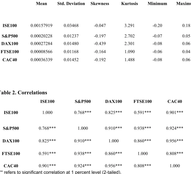
Table 1 reports the characteristics of the data set. It reports the average daily returns

and the standard deviations of returns calculated as the log differences of the national

stock indices. All of the five national markets have positive average daily returns.

ISE 100 has the highest standard deviation of return among the five markets. This

result is consistent with the view that the emerging markets have higher volatility

than the developed markets (Harvey, 1991). The last two columns of the table show

the skewness and kurtosis coefficients. All national index return series have

skewness coefficients of less than –0.5, indicating negative skewness. ISE 100 has

the highest kurtosis coefficient (3.291) which is greater than 3 indicating

leptokurtosis.

In table 2 correlations of the all possible index pairs are calculated. Results

illustrate that all of the correlation coefficients are positive and significant at 1

percent level. The smallest correlation coefficient is equal to 0.591 which is between

ISE100 and FTSE100. All possible correlation coefficients between two developed

stock markets is greater than 0.8.

(26)

Table 1. Descriptive Statistics

Mean Std. Deviation Skewness Kurtosis Minimum Maximum

ISE100 0.00157919 0.03468 -0.047 3.291 -0.20 0.18 S&P500 0.00020228 0.01237 -0.197 2.702 -0.07 0.05 DAX100 0.00027284 0.01480 -0.439 2.301 -0.08 0.06 FTSE100 0.00008566 0.01168 -0.164 1.090 -0.06 0.04 CAC40 0.00036339 0.01452 -0.192 1.488 -0.08 0.06

Table 2. Correlations

ISE100 S&P500 DAX100 FTSE100 CAC40

ISE100 1.000 0.768*** 0.825*** 0.591*** 0.901***

S&P500 0.768*** 1.000 0.910*** 0.938*** 0.924***

DAX100 0.825*** 0.910*** 1.000 0.860*** 0.956***

FTSE100 0.591*** 0.938*** 0.860*** 1.000 0.808***

CAC40 0.901*** 0.924*** 0.956*** 0.808*** 1.000

*** refers to significant correlation at 1 percent level (2-tailed).

5.1 Unit Root Tests

The stationarity of the natural logarithmic index series are examined by the

Dickey-Fuller and the Phillips-Perron Unit Root Tests at levels and first differences.

DF and PP test results are calculated with the constant, constant and trend, no

constant and no trend specifications. Columns of I (0) indicate the results of the tests

at levels and columns of I (1) indicates the results of the test at first differences.

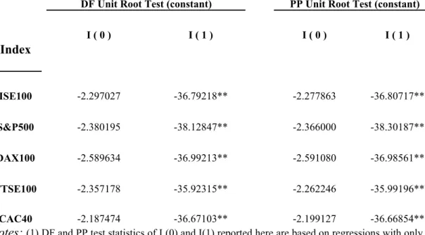
Table 3 reports the results of DF and PP Unit Root Tests with only constant

specification.

(27)

Table 3. Results of the Dickey-Fuller (DF) and the Phillips-Perron Unit Root

Tests

DF Unit Root Test (constant) PP Unit Root Test (constant)

I ( 0 ) I ( 1 ) I ( 0 ) I ( 1 )

Index

ISE100 -2.297027 -36.79218** -2.277863 -36.80717** S&P500 -2.380195 -38.12847** -2.366000 -38.30187** DAX100 -2.589634 -36.99213** -2.591080 -36.98561** FTSE100 -2.357178 -35.92315** -2.262246 -35.99196**

CAC40 -2.187474 -36.67103** -2.199127 -36.66854**

Notes:

(1) DF and PP test statistics of I (0) and I(1) reported here are based on regressions with only constant specification. (2) The numbers on the table refer to

βo

coefficients. (3) * and ** refer to significance levels 5% and 1% respectively.

Table 4. Results of the Dickey-Fuller (DF) and the Phillips-Perron Unit Root

Tests

DF Unit Root Test (constant, trend) PP Unit Root Test (constant, trend)

I ( 0 ) I ( 1 ) I ( 0 ) I ( 1 ) Index ISE100 -1.613590 -36.85104** -1.678458 -36.85941** S&P500 -1.372095 -38.25125** -1.192851 -38.48578** DAX100 -1.620440 -37.10602** -1.625311 -37.09832** FTSE100 -1.832797 -36.00751** -1.657926 -36.12013** CAC40 -0.807644 -36.79407** -0.704578 -36.81652**

Notes:

(1) ADF and PP test statistics of I (0) and I(1) reported here are based on regressions with constant and trend specification. (2) The numbers on the table refer to

βo

Table 4 reports the results of DF and PP Unit Root Tests with both constant and

trend specifications.

(28)

Table 5. Results of the Dickey-Fuller (DF) and the Phillips-Perron Unit Root

Tests

DF Unit Root Test (no constant, no trend) PP Unit Root Test (no constant, no trend)

I ( 0 ) I ( 1 ) I ( 0 ) I ( 1 ) Index ISE100 1.512540 -36.73196** 1.451425 -36.75473** S&P500 0.559327 -38.13115** 0.621642 -38.30155** DAX100 0.630303 -36.99194** 0.624644 -36.98583** FTSE100 0.243962 -35.93343** 0.272435 -36.00306** CAC40 0.873583 -36.65917** 0.912561 -36.65380**

Notes:

(1) DF and PP test statistics of I (0) and I(1) reported here are based on regressions without constant and trend specification. (2) The numbers on the table refer to

βo

ADF and PP tests report that all of the logarithmic national stock index series

have unit roots at levels, that is, they are not I (0) at 5 percent significance in all

specifications. Five market indices are not stationary at levels. However, the DF and

PP tests applied on the first differenced series does not exhibit a unit root, that is, all

series are I (1) at 1 percent significance level in all specifications.

So both Dickey-Fuller and Phillips-Perron Unit Root Tests showed that all

logarithmic national stock index series are not stationary at levels, but their first

order differences are stationary at 1 percent significance. There is no difference

between the results of DF and PP Unit Root Tests for our sample.

(29)

5.2 Cointegration Tests

Since all index series are I (1), cointegration analysis is conducted by using the

cointegration technique developed by Engle and Granger (1987). MacKinnon`s

(1993) critical values are used to test the residuals of the regressions. Dickey-Fuller

Unit Root Test results for the OLS residuals at leves are provided. Table 6 reports

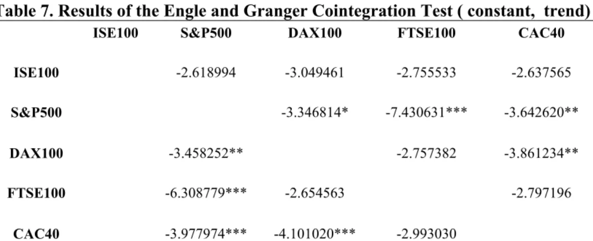
the results of cointegration tests with constant specification. Table 7 reports the

results of cointegration tests with both constant and trend specifications.

Table 6. Results of the Engle and Granger Cointegration Test (constant)

ISE100 S&P500 DAX100 FTSE100 CAC40 ISE100 -1.479348 -1.639973 -1.075072 -2.077016 S&P500 -3.349329** -4.721552*** -3.250072**

DAX100 -3.450147*** -2.218268 -3.099909**

FTSE100 -4.800465*** -2.237025 -1.866252

CAC40 -3.055931** -2.770893* -1.258668

Notes:

(1) DF test statistics of OLS residuals at levels with constant specification. (2) The numbers on the table refer to

ψ

o coefficients. (3) *, ** and *** refer to significance levels 10%, 5% and 1% respectively.

Table 7. Results of the Engle and Granger Cointegration Test ( constant, trend)

ISE100 S&P500 DAX100 FTSE100 CAC40 ISE100 -2.618994 -3.049461 -2.755533 -2.637565 S&P500 -3.346814* -7.430631*** -3.642620**

DAX100 -3.458252** -2.757382 -3.861234**

FTSE100 -6.308779*** -2.654563 -2.797196

CAC40 -3.977974*** -4.101020*** -2.993030

Notes:

(1) DF test statistics of OLS residuals at levels with constant and trend specification. (2) The numbers on the table refer to

ψ

(30)

Table 8 reports the results of cointegration tests without constant and trend

specifications.

Table 8. Results of the Engle and Granger Cointegration Test (no constant, no

trend)

ISE100 S&P500 DAX100 FTSE100 CAC40 ISE100 -1.480576 -1.641224* -1.076369 -2.078369** S&P500 -3.350509*** -4.723362*** -3.251238***

DAX100 -3.451331*** -2.219212** -3.100898***

FTSE100 -4.802322*** -2.238054** -1.867169*

CAC40 -3.057101*** -2.771877*** -1.259559

Notes:

(1) DF test statistics of OLS residuals at levels without constant and trend specification. (2) The numbers on the table refer to

ψ

All three types of test results report the cointegration between stock market index

series according to the different specifications. Although there are differences

among the DF test results of the OLS regression results according to the trend and

intercept (constant) specifications, we can say that all three types of DF test results

are similar. By looking at the three tables, we can say that table 8, which gives the

DF test results without constant and trend specifications, has the most comprehensive

results among three tables.

Table 8 reports that Turkey and France are cointegrated at 5 percent significance

level. It also reports that cointegration exist between Turkey and Germany at 10

percent significance. These results suggest that the Turkish stock market is

influenced significantly by the French and German markets in the long-run.

(31)

All three tables report that the US stock market and each of the European stock

markets are highly cointegrated. The US stock market influence all three European

markets at 1 percent significance level. In contrast, all three European markets

influence the US stock market individually at 1 percent significance level.

On the other hand, table 8 reports that the null hypothesis of no cointegration

between pairs of European stock markets is rejected. Germany, UK and France are

cointegrated with each other at different significance levels. France and Germany

are highly cointegrated at 1 percent significance level. Both markets are influenced

by each other in the long-run. UK and Germany are cointegrated at 5 percent

significance level. The UK market is influenced by the German market in the

long-run and vice versa. On the other hand, UK and France are not strongly cointegrated.

Table 8 indicates that the null hypothesis of the UK stock market is independent of

the French stock market is rejected at 10 percent significance level. But the null

hypothesis of the French stock market is independent of the UK stock market is not

rejected. In other words, UK is influenced by France but not vice versa.

5.3 Vector Error Correction (VEC)

The findings of cointegration tests indicate that the null hypothesis of no

cointegration between the pairs of developed stock markets (the US and European

markets) is rejected. The Turkish stock market as an emerging market appears to be

cointegrated with the French and German stock markets. According to the Granger`s

representation theorem, if two variables are cointegrated then there always exist an

error correction formulation of the dynamic model and vice versa. So, we next

(32)

equations (11 and 12). The term

Z

t-1,

used in the vector error correction regressions

was obtained from the OLS estimation of the cointegration equation (7). In long-run

equilibrium, the error correction term (

Z

t-1

)

is zero. However, if Xt and Yt series

deviated from long-run equilibrium last period, the error correction term is nonzero

and each variable adjusts to partially the equilibrium relation. The results of the

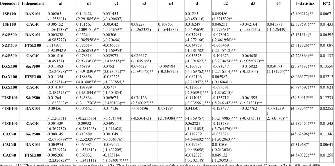
vector error correction equations are reported in Table 9.

The sign, significance and size of the coefficient a

1

shows the speed of

adjustment how the dependent series changes in response to disequilibrium in the

long-run. In table 9, if a

1

(the coefficient of the error-correction term) has a negative

value and its “t-value” is significant, it indicates the speed of adjustment of the

dependent index series (Yt in equation 11) at day t to correct the previous

disequilibrium at day t-1.

This result implies that the equilibrium error can be used to predict next period`s

index changes in that stock market. Error correction analysis also yields information

about the “short run” influence of the change in one market on the performance of

another market. The t-ratios of c1, c2, c3, c4 indicates a short-run relationship when

at least one of the “t-ratio” of these coefficients is significant.

We will analyze the relations between Turkey and developed markets first. Next,

the relations between the US market and the European markets will be analyzed.

Finally, we will examine the relations among the three European markets.

(33)

Table 9. Vector Error Correction Results

Dependent Independent a1 c1 c2 c3 c4 d1 d2 d3 d4 F-statistics R^2

ISE100 DAX100 -0.00265 0.146428 0.031455 (-1.255801) (2.291885)** (-0.490607) ISE100 CAC40 -0.005152 0.131563 0.003042 0.08227 (-1.861233)* (2.009171)** (-0.046597) S&P500 DAX100 -0.003838 0.05264 0.00506 (-0.985777) (1.985958)** (-0.20464) S&P500 FTSE100 0.014931 0.075014 -0.036059 (1.923942)* (2.265873)** (-1.160953) S&P500 CAC40 -0.001516 0.078515 0.039972 0.026647 (-0.49137) (2.933363)*** (1.476518)** DAX100 S&P500 -0.011483 0.46889 0.0752 (-2.624898)*** (13.91039)*** (2.053032)** DAX100 FTSE100 -0.011354 0.188856 -0.082273 (-3.027314)*** (4.018067)*** (-1.737885)* DAX100 CAC40 -0.014197 0.193939 0.05717 (-2.182393)** (4.451844)*** (-1.304834) FTSE100 S&P500 -0.01264 0.343834 0.069675 0.070126 (-1.823263)* (13.11776)*** (2.480106)** (2.540327)** FTSE100 DAX100 -0.00456 0.006652 0.017136 (-1.526351) (-0.225596) (-0.578144) FTSE100 CAC40 -0.001439 -0.00932 0.049811 (-0.767737) (-0.284263) (-1.518628) CAC40 S&P500 -0.009145 0.413689 0.001049 (-2.678679)*** (12.52329)*** (-0.030176) CAC40 DAX100 -0.004974 0.064985 -0.069092 (-0.774972) (-1.531613) (-1.633209) CAC40 FTSE100 -0.005206 0.068032 -0.153814 (-2.232682)** (-1.341111) (-3.030017)*** 0.01225 0.049486 (2.406212)** 0.0067 (-0.450116) (1.821532)* 0.107567 0.016249 0.048251 -0.042164 0.041571 (2.579591)*** 0.01433 (-1.262332) (-1.644585) (-0.596659) (1.77563)* (-1.551222) (-1.526439) -0.037981 -0.078012 (2.131914)* 0.00595 (-1.272166) (-2.461956)** -0.034759 -0.065469 (3.917826)*** 0.01087 (-1.181782) (-2.115718)** -0.053575 -0.104673 -0.064638 (2.726864)** 0.01137 (-1.059168) (-1.791827)* (-3.270874)*** (-2.056077)** 0.076623 -0.008484 -0.160723 -0.083247 -0.015822 0.059173 (27.84133)*** 0.13559 (2.094375)** (-0.236795) (-5.369762)*** (-2.736314)*** (-0.52106) (2.131705)** -0.082196 0.005982 (8.066377)*** 0.02213 (-2.210572)** (-0.160881) -0.127678 -0.079591 (6.984093)*** 0.01921 (-2.96894)*** (-1.856213)* -0.111013 -0.155712 -0.061595 (34.5991)*** 0.12731 (-3.735561)*** (-5.246347)*** (-2.21531)** -0.015896 0.081994 0.043501 -0.123477 -0.027762 -0.081289 (4.08904)*** 0.02252 (-0.536473) (2.789084)*** (-1.159767) (-3.274985)*** (-0.737361) (-2.160176)** 0.062828 -0.153583 (5.587451)*** 0.01543 (-1.541085) (-3.764576)*** -0.119739 -0.053821 (45.62696)*** 0.11346 (-4.044602)*** (-1.932863)** -0.019284 0.010506 (2.31968)* 0.00647 (-0.448658) (-0.243036) -0.012327 0.049132 (4.540322)*** 0.01258 (-0.302148) (-1.203831)

(34)

Table 9 reveals that when a deviation from the equilibrium occurs, Istanbul Stock

Exchange reacts to make the necessary adjustment for the equilibrium in the long-run

between Turkey and France. Coefficients of c1 show that both Germany and France

have important short-run effects on the Turkish market.

When a deviation occurs from the equilibrium between the US market and any of

the European markets, the US market gives response only to the UK market to make

the necessary adjustment to remove the disequilibrium. According to table 9,

Germany, UK and France have significant a

1

coefficients which are -0.0115, -0.0126,

-0.0092 respectively to response the disequilibrim with US. For example, when a

deviation occurs between Germany and US at day t-1, 1.15% of the disequilibrium is

removed by the reaction in Germany at day t and no reaction is observed from US.

All three European markets react significantly to restore the equilibrium relation with

US. Table 9 reports that the European markets have significant short-run impacts on

the US market. The coefficients of c1, c2, c3 which reports the impact of US on the

European markets in the short-run are usually large and significant. This means that

US exerts substantial amount of influence on the European markets.

When a deviation from long-run equilibrium occurs between Germany and UK or

Germany and France, table 9 reports that Germany reacts to correct the deviation. In

other words, Germany gives responses partially to restore both of the equilibriums.

When a deviation from long-run equilibrium occurs between UK and Germany or

UK and France, UK does not give any response to make the necessary adjustment to

remove the previous disequilibrium. When a deviation from long run equilibrium is

observed between France and UK, the French stock market reacts to remove the

(35)

fraction of the previous disequilibrium. In contrast, the French market does not react

for the deviation from long-run equilibrium between France and Germany.

Among the European markets, France and UK have significant impacts on

Germany in the short-run. UK is influenced by the German stock market in the

short-run. France does not have a short-run impact on UK. Table 9 also reports that,

France is influenced by UK in the short-run. Germany does not have a significant

short-run impact on France.

(36)

6. CONCLUSION

Today, we are living in a world environment in which we have much freer

international movement of capital flows and information. The interactions and

integration among the World`s stock markets have received much attention from

economists and investors.

The aim of this thesis is to analyze long-run and short-run linkages and dynamic

interactions among five stock exchanges which consists of one emerging and four

developed markets. The emerging stock market is Istanbul Stock Exchange, and the

developed markets are New York, Frankfurt, London and Paris. Cointegration

analysis and vector error correction model were used. Daily stock markets indices at

closing time were used for the period between January 1997 and June 2002. The

sample consists of 1433 daily observations.

Tests of stationary allow us to conclude that all time series are non-stationary at

levels at 5 percent significance, but first differenced series are stationary. Thus, all

national stock market index series are integrated of order one, I(1), and the use of

cointegration analysis and error correction model is appropriate to test for long-run

and short-run relationships between stock markets.

As an emerging and young market, Turkey is influenced significantly by the

French and German markets both in the long-run and short-run. Moreover, when a

(37)

deviation from the equilibrium occurs between Turkey and France, Turkey reacts to

make the necessary adjustment for the equilibrium in the long-run.

The US market and each of the three European markets are highly cointegrated.

The European markets are influenced by the US market both in the long-run and

short-run and vice versa. When a deviation from long-run equilibrium occurs

between US and any of the three European countries, error correction results point

out that index adjustment process occurs on that European stock market. US only

gives reactions to UK to restore the equilibrium in the long-run. This result is

consistent with the view that innovations in the US market are rapidly transmitted to

other markets in a clearly recognizable fashion. Our results also prove that US is the

most influential market among the four developed markets.

All possible pairs of three European markets are cointegrated and this shows the

existence of links between any market pair. This can be explained by the fact that

the three countries are members of the European Union. When a deviation from

long-run equilibrium occurs between Germany and UK or Germany and France,

index adjustment process occurs only on the German stock market but not on the

other stock market. When a deviation from long-run equilibrium occurs between

France and UK, index adjustment process occurs only on the French stock market

but not on the UK market. UK seems to be the most influential market among the

three European countries. The reason for this result can be explained by the fact that

UK has the largest stock exchange in Europe.

(38)

Although cointegration exists between the pairs of developed markets, this does

not indicate useful and profitable predictability. One should be careful in

considering the closing time differences of these stock markets. The error correction

may as well be the result of these time differences.

As a result, the markets have been globalized. Especially developed stock

markets are not independent from each other but move together. Previous studies

have made a strong case for international portfolio diversification to reduce risk. And

it makes sense for the investors. However, this study reports that national stock

markets lack interdependence is rejected for the examined stock markets because of

significant reported short-run and long-run relationships. Therefore, diversification

among national markets will not reduce the portfolio risk substantially.

(39)

BIBLIOGRAPHY

Arshanapalli, B., & J. Doukas. 1993. “International Stock Market Linkages:

Evidence from the pre- and post-October 1987 Period,” Journal of Banking and

Finance 17, 193-208.

Bayar, A. 2002. “Cointegration Between The French and The German Stock

Markets: Evidence From Cross-Listed French Stocks,” Ph. D. Thesis, Bilkent

University, 86-105.

Becker, K. G., Finnerty, J. E., & M. Gupta. 1990. “The Intertemporal Relation

Between the U.S. and Japanese Stock Markets,” The Journal of Finance XLV (4),

1297-1306.

Davidson, R., & J. G. MacKinnon. 1993. “Estimation and Inference in

Econometrics,” Oxford University Press, 700-730.

Dickey, D.A., & W. A. Fuller. 1981. “Likelihood Ratio Statistics For Autoregressive

Time Series With A Unit Root,” Econometria 49 (4), 1057-1072.

Engle, R. F., & C. W. J. Granger. 1987. “Co-Integration and Error Correction:

Representation, Estimation, and Testing,” Econometrica 55 (2), 251-276.

Eun, C. S., & S. Shim. 1989. “International Transmission of Stock Market

Movements,” Journal of Financial and Quantitative Analysis 24 (2), 241-256.

Furstenberg, G. M. V., & B. N. Jeon. 1989. “International Stock Price Movements:

Links and Messages,” Brookings Papers on Economic Activity 1989 (1), 168-179.

Gerrits, R. 1995. “Short- and Long-Term Links Among European And US Stock

(40)

Hakim, S. R. 2001. “Price Linkages and Integration Of The Cairo Stock Exhange,”

Working Paper, Energetix Corp., Houston, Texas.

Harris, F. H., Mclnish, T. H., Shoesmith, G.L., & R. A. Wood. 1995.

“Cointegration, Error Correction, and Price Discovery on Informationally Linked

Security Markets,” Journal Of Financial and Quantitative Analysis 30 (4), 563-579.

Harvey, C. R. 1991. “The World Price of Covariance Risk,” The Journal of Finance

46(1), 111-157.

MacKinnon, J.G. 1991. “Critical Values for Cointegration Tests,” Chapter 13 in

Long-run Economic Relationships: Readings in Cointegration, edited by R.F.Engle

and C.W.J. Granger, Oxford University Press.

Malliaris, A. G., & J. Urrita. 1992. “The International Crash of October 1987:

Causality Tests,” Journal of Finance and Quantitative Analysis 27, 353-364.

Muradoglu, G., & K. Metin. 1999. “Forecasting Integrated World Stock Markets

Using International Co-Movements,” Working Paper Bilkent University.

Mukherjee, C., White, H., & M. Wuyts. 1998. “Econometrics and Data Analysis for

Developing Countries,” Routledge Press, New York.

Phillips, P.C.B., & P. Perron. 1988. “Testing for a Unit Root in Time Series

Regression,” Biometrika 75, 335–346.

(41)

ISE 100 (IN LOG)

0.00000000 2.00000000 4.00000000 6.00000000 8.00000000 10.00000000 12.00000000 01.01.1997 01.03.1997 01.05.1997 01.07.1997 01.09.1997 01.11.1997 01.01.1998 01.03.1998 01.05.1998 01.07.1998 01.09.1998 01.11.1998 01.01.1999 01.03.1999 01.05.1999 01.07.1999 01.09.1999 01.11.1999 01.01.2000 01.03.2000 01.05.2000 01.07.2000 01.09.2000 01.11.2000 01.01.2001 01.03.2001 01.05.2001 01.07.2001 01.09.2001 01.11.2001 01.01.2002 01.03.2002 01.05.2002

(42)

S&P 500 (IN LOG)

6.20000000 6.40000000 6.60000000 6.80000000 7.00000000 7.20000000 7.40000000 01.01.1997 01.03.1997 01.05.1997 01.07.1997 01.09.1997 01.11.1997 01.01.1998 01.03.1998 01.05.1998 01.07.1998 01.09.1998 01.11.1998 01.01.1999 01.03.1999 01.05.1999 01.07.1999 01.09.1999 01.11.1999 01.01.2000 01.03.2000 01.05.2000 01.07.2000 01.09.2000 01.11.2000 01.01.2001 01.03.2001 01.05.2001 01.07.2001 01.09.2001 01.11.2001 01.01.2002 01.03.2002 01.05.2002

(43)

DAX 100 (IN LOG)

6.60000000 6.80000000 7.00000000 7.20000000 7.40000000 7.60000000 7.80000000 8.00000000 8.20000000 8.40000000

(44)

FTSE 100 (IN LOG)

8.00000000 8.10000000 8.20000000 8.30000000 8.40000000 8.50000000 8.60000000 8.70000000 8.80000000 8.90000000 01.01.1997 01.03.1997 01.05.1997 01.07.1997 01.09.1997 01.11.1997 01.01.1998 01.03.1998 01.05.1998 01.07.1998 01.09.1998 01.11.1998 01.01.1999 01.03.1999 01.05.1999 01.07.1999 01.09.1999 01.11.1999 01.01.2000 01.03.2000 01.05.2000 01.07.2000 01.09.2000 01.11.2000 01.01.2001 01.03.2001 01.05.2001 01.07.2001 01.09.2001 01.11.2001 01.01.2002 01.03.2002 01.05.2002

(45)

CAC-40 (IN LOG)

7.00000000 7.20000000 7.40000000 7.60000000 7.80000000 8.00000000 8.20000000 8.40000000 8.60000000 8.80000000 9.00000000 01.01.1997 01.03.1997 01.05.1997 01.07.1997 01.09.1997 01.11.1997 01.01.1998 01.03.1998 01.05.1998 01.07.1998 01.09.1998 01.11.1998 01.01.1999 01.03.1999 01.05.1999 01.07.1999 01.09.1999 01.11.1999 01.01.2000 01.03.2000 01.05.2000 01.07.2000 01.09.2000 01.11.2000 01.01.2001 01.03.2001 01.05.2001 01.07.2001 01.09.2001 01.11.2001 01.01.2002 01.03.2002 01.05.2002