Available online at http://www.academicjournals.org/ajar DOI: 10.5897/AJAR09.177
ISSN 1991-637X © 2010 Academic Journals
Full Length Research Paper
Determination of the best blackberry cultivar using
various statistical techniques
Ecevit Eyduran
1*, S. Peral Eyduran
2, Khalid Mahmood Khawar
3andY. Sabit Agaoglu
41Biometry Genetics Unit, Department of Animal Science, Faculty of Agriculture, Igdir University, 76000 Igdir, Turkey, 2Department of Horticulture, Faculty of Agriculture, Igdir University, 76000 Igdir, Turkey.
3Department of Field Crops, Faculty of Agriculture, University of Ankara, 06110 Ankara, Turkey. 4Department of Horticulture, Faculty of Agriculture, University of Ankara, 06110 Ankara, Turkey.
Accepted 30 September, 2009
This study was conducted to determine the best blackberry cultivar using jointly various statistical techniques such as Chi-Square, G, and Correspondence statistics. For this aim, data of pomological traits such as fruit weight, cane number, cane diameter, cane height, cane yield per plant of Ness, Cherokee, Arapaho, Chester Thornless, Navaho, Black Satin, Dirksen Thornless and Jumbo cultivars were collected during 2002-2006. With respect to chi-square and G statistics, associations between cultivar and each pomological trait (fruit weight, cane number, cane diameter, cane height, and cane yield per plant) were found more significant (P < 0.0001). The relationship between year and cane number was significant (P < 0.0001 and year and cane diameter was significant (P < 0.05). The highest cane number was produced in 2004, followed by 2005. The relationship between fruit weight and cane diameter or cane yield per plant were more significant (P < 0.0001). Although Blacksatin and Jumbo blackberry cultivars had the highest cane number, Chester Thornless from blackberry cultivars had the highest cane diameter, the highest cane yield per plant and the highest fruit weight. It was concluded that Chester Thornless cultivar was the most appropriate cultivar for Central Anatolia region.
Key words: Adaptation, blackberry, cane, fruit, Chi-square statistic, G statistic, correspondence analysis.
INTRODUCTION
The blackberry is an aggregate fruit from, genus Rubus in the family Rosaceae. They are perennial plants and bear biennial stems ("canes") from the perennial root system. They do not produce flowers during first year, which are produced during second year on the stems that does not grow longer, but the flower buds break to produce flowering laterals.
In horticulture of blackberry, the effects of yearly environmental and genotype (cultivar) factors have a variable effect on pomological traits such as fruit weight, cane diameter, cane length, cane height, cane per plant, and others (Atila et al., 2006a; Atila et al., 2006b; Eyduran and Agaoglu, 2006; Eyduran et al., 2007). These factor effects are generally examined by using Analysis of Variance (ANOVA) in the adaptation and other
studies (genetic improvement; determination of chemical
*Corresponding author E-mail: [email protected].
components) on blackberries (Strik et al., 1996; Finn et al., 1999; Siriwoharn et al., 2005; Clark et al., 2005; Yorgey and Finn, 2005; Connor et al., 2005a, b; Finn et al., 2005a, b, c, d, e). However, there are no studies on selection of the best Blackberry cultivars, using the effects of relationships between pomological traits and their effects on each other. These are generally calculated using Correspon-dence Analysis (CA), Chi-Square and G statistics can be used jointly for obtaining different information. Using CA and other statistical techniques could be equally important for horticulture of this plant.
In general, Chi-Square, Likelihood Chi-Square, Fisher’s Exact and Log-linear, Logistic Regression, and Corres-pondence are used in statistical analysis of contingency (two-way) tables (Everitt, 1992; Baspınar and Mendes, 2000; Eyduran et al., 2005a; Eyduran and Ozdemir, 2007). Chi-square, Likelihood Chi-square and Fisher’s Exact statistics gives an idea about whether association between categorical variables is significant (Dugan’s,
Eyduran et al. 899
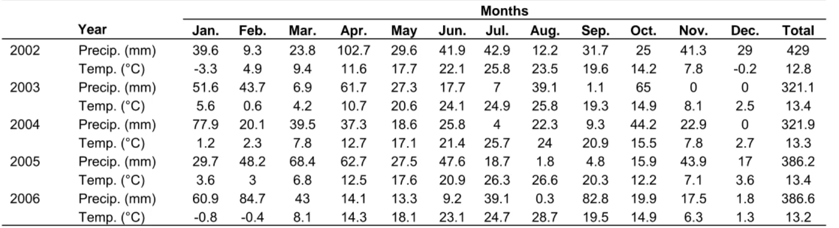
Table 1. Monthly temperature and preciption in each year for Ankara ecology.
Year
Months
Jan. Feb. Mar. Apr. May Jun. Jul. Aug. Sep. Oct. Nov. Dec. Total
2002 Precip. (mm) 39.6 9.3 23.8 102.7 29.6 41.9 42.9 12.2 31.7 25 41.3 29 429 Temp. (°C) -3.3 4.9 9.4 11.6 17.7 22.1 25.8 23.5 19.6 14.2 7.8 -0.2 12.8 2003 Precip. (mm) 51.6 43.7 6.9 61.7 27.3 17.7 7 39.1 1.1 65 0 0 321.1 Temp. (°C) 5.6 0.6 4.2 10.7 20.6 24.1 24.9 25.8 19.3 14.9 8.1 2.5 13.4 2004 Precip. (mm) 77.9 20.1 39.5 37.3 18.6 25.8 4 22.3 9.3 44.2 22.9 0 321.9 Temp. (°C) 1.2 2.3 7.8 12.7 17.1 21.4 25.7 24 20.9 15.5 7.8 2.7 13.3 2005 Precip. (mm) 29.7 48.2 68.4 62.7 27.5 47.6 18.7 1.8 4.8 15.9 43.9 17 386.2 Temp. (°C) 3.6 3 6.8 12.5 17.6 20.9 26.3 26.6 20.3 12.2 7.1 3.6 13.4 2006 Precip. (mm) 60.9 84.7 43 14.1 13.3 9.2 39.1 0.3 82.8 19.9 17.5 1.8 386.6 Temp. (°C) -0.8 -0.4 8.1 14.3 18.1 23.1 24.7 28.7 19.5 14.9 6.3 1.3 13.2 State Meteorology Instute, Ankara 2006.
1983; Everitt, 1992; Sokal and Rohlf, 1996), but correspondence analysis provides more information than others because it visualizes interaction with levels of categorical variables (Keskin, 2001).
As regards the best choice between Chi-Square and Likelihood Chi-Square statistics, many authors reported that observed frequency for each cell of contingency tables should be at least five. If any cells frequency were less than five, Likelihood Ratio Chi-square statistic might be more superior to Chi-square statistic, whereas Agresti (2002) reported that Chi-square has more advantageous than other if
n
/
r c
*
5
where n, total sample size; r, row number and c, column number. Eyduran et al. (2006b) reported that SAS program gave warning “Chi-square may not be valid statistic” when more than 20% of cells expected counts less than five. In addition, it was well-known that both statistics values increases proba-bility of being resemble on each other as total sample size increases (Sokal and Rohlf, 1996; Agresti, 2002; Eyduran and Ozdemir, 2005; Ozdemir et al., 2006a).It was stated by many authors that in order to deter-mine the best statistic, power analysis for Chi-Square, Likelihood Chi-Square statistics should be performed under every condition and the statistic with a power of at least 80% should be desired (Agresti, 2002; Eyduran and Ozdemir, 2005).
Contrary to Chi-Square and Likelihood Chi-Square statistics, Correspondence Analysis (which has been widely used for studies on genetics, ecology, economy, marketing, plant and animal breeding) might help to determine the relationship that categories of one variable can be interacted with each other and categories of other variable. Its advantages have no assumptions and hypo-thesis on distribution of data set (Gauch, 1982; Eyduran et al., 2006c; Akturk et al., 2007).
The first aim of this study is to determine the best adaptation performance among 8 blackberry cultivars to
recommend the best one(s) to blackberry farmers and breeders for use in the continental climate of Central Anatolia, Turkey. The second one is to determine amount of association between pomological traits of 8 blackberry cultivars using power analysis of Chi-Square, Likelihood Chi-Square statistics, using special macro written in SAS program reported by Ozdemir et al. (2006b). The third aim is to show interaction among categories graphically for two variables (pomological traits) using Correspondence Analysis.
MATERIALS AND METHODS
The adaptation experiment was carried out on eight blackberry cultivars Ness, Cherokee, Arapaho, Chester Thornless, Navaho, Black Satin, Dirksen Thornless and Jumbo at Farm of Horticulture Research and Application, Faculty of Agriculture, University of Ankara during 2002-2006, located at 32°52΄ north, 39°56΄ east, continental climate with wide variations in temperature, both between seasons and between different times of the day. Its summers are hot and dry, but its winters are cold and wet. Meteorological data of experimental site is given Table 1.
Two rows for each blackberry shrub plant set at 2 x 2 m spacing were harvested during August-September interval. All the traits had 120 observations in the adaptation experiment (8 cultivars x 5 years x 3 replications).
Berries were weighed fresh (fruit) and averages of fruit weight were calculated from 30-sample randomly selected from three plots for each blackberry cultivars. Cane weight, diameter, and height of shrub plants were calculated as recommended by Eyduran et al. (2007). Descriptive statistics of all traits are given in Table 2.
Variable structures
Categorical variables
Year (2002, 2003, 2004, 2005, and 2006) and Cultivar variables (Ness, Cherokee, Arapaho, Chester Thornless, Navaho, Black Satin, Dirksen Thornless, and Jumbo) are naturally ones with categorical structure.
Table 2. Descriptive statistics of pomological traits in blackberry.
Pomological trait N Mean Standard error Minimum Maximum
Fruit Weight (FW) 120 3.44 0.10 1.00 5.50
Cane Number (CN) 120 10.65 0.20 6.60 15.2
Cane yield per plant (CYP) 120 104.17 4.17 52.60 210.7
Cane Diameter (CD) 120 17.81 0.35 9.0 28.4
Cane Height (CH) 120 226.93 3.52 100 300
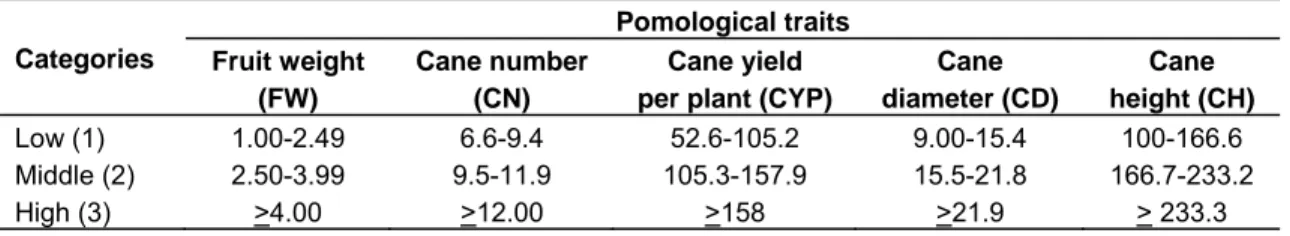
Table 3. The cut-off values of pomological traits. Categories Pomological traits Fruit weight (FW) Cane number (CN) Cane yield per plant (CYP)
Cane diameter (CD) Cane height (CH) Low (1) 1.00-2.49 6.6-9.4 52.6-105.2 9.00-15.4 100-166.6 Middle (2) 2.50-3.99 9.5-11.9 105.3-157.9 15.5-21.8 166.7-233.2 High (3) >4.00 >12.00 >158 >21.9 > 233.3
Grouped (Categorized) variables
Pomological traits such as Fruit weight, Cane number, Cane yield per plant, Cane diameter, Cane height have generally variables with continuous structure. However, these traits can be transformed from Continuous structure to categorical one. In the adaptation experiment, the pomological traits have transformed as follows: after averages of these traits were found, all observations for each trait were categorized to 3 groups; namely, little (1), middle (2), more (3). The cut-off values of all traits (grouped variables) are presented in Table 3. These were graded and coded into three categories that is, (1) little with fruit weight of 1.-2.49 g, (2) middle with fruit weight of 2.50-3.99 g (3) more with fruit weight of >4.00 g.
The notation of Chi-Square (1) and Likelihood Ratio Chi-Square statistics (2) are written as follows (Everitt, 1992; Agresti, 2002; Eyduran and Ozdemir, 2005):
i i f f f 2 2 (1) i f f f G 2 .ln (2)
Where, f, observed frequency and fi ,expected frequency.
Power theory for Chi-square and G statistics
Assume that H0 is the same to model M for a contingency table. Let
i
indicate the true probability in ith cell and Leti
(M) represent the value to which the Maximum likelihood (ML) estimate
ˆi for model M converges, where
i
i(M)1. For multinomial sample of size n, the non-centrality parameter for Chi-square (3) can be expressed as follows:
i i i i M M n ) ( ) ( 2
(3)Expression 3 is the similar form of Chi-square statistics, with the sample proportion pi and
i(M)in place of
ˆi. The non-centralityparameter for Likelihood Ratio Chi-Square Statistics (4) can be written in this manner:
i i i i M n ) ( log 2
(4)In order to obtain reliable results from both statistics, one should achieve a power value of at least 80% (Agresti, 2002; Ozdemir et al., 2006a, b). The highest value for power analysis of both statistics is 1. The data were analyzed using Minitab ((Minitab, 2007; released version 15) and SAS (2006, version 9.0) package programs. Power Analysis Chi-square and G statistics were performed using a special SAS macro at web site:
( http://ftp.sas.com/techsup/download/stat/powerrxc.html) Correspondence analysis
Correspondence analysis (CA) is called a variety of names in the literature: Contingency table analysis, RQ-technique, reciprocal averaging, reciprocal ordering, dual scaling, optimal scaling, optimal scoring, and quantification method or homogeneity analysis (Statsoft, 1997; Eyduran et al., 2006b). CA, which is analogous to Principle Components, is a descriptive analysis technique which is designed to analyze two-way and multi-way tables containing measures of correspondence between the row and column variables (Ender, 2005; Gauch, 1982). In other word, it supplies a statistic method for representing data in a Euclidean space so that the results can be visually observed for structure.
The Pearson Chi-square Statistic,
2p, is a sum of squared ij
values, which are computed every cell ij of the contingency table. Eachij
value is the standardized residual of a frequency fijthat there is no relationship between the rows and the columns of the table. For each cell:
j i j i ij ij ij ij ij p p p p p f E E O (5)
CA is based on the matrix Q:
j i j i ij ij p p p p p q Q (6)Where; the
q
ijvalues are the basis of CA and only differ from
ij’s by a constantf
. Thus, all of the eigenvalues become equal to < 1.The sum of squares of all the values in the
2,
q
ijQ
measures the total inertia inQ
. It is also equal to the sum of all of the eigenvalues to be extracted.Singular value decomposition (SVD) is then applied to the
Q
matrix. While this process computationally a bit involved, the similar response more straightforwardly derived by applying eigenvalue analysis to covariance matrixQ
Q
, which would produce the matrices of eigenvalues
and eigenvectors U. OnceU is acquired, one can easily solve for
Uˆ
because of the relationship:
12ˆ
U
Q
U
rxc (7)The process always yields one null eigenvalue owing to the centering in the determination of
Q
.Matrices U and
Uˆ
may be used to plot the positions of the row and column vectors in two separate scatter diagrams. For joint plots, different scaling types of the row and column scores have been suggested.Matrices U and
Uˆ
can be weighted by inverse of the square roots of the column and row scores, which were written out in diagonal matrices
12 j
p
D with dimension cxc and
12 i
p
D
with dimension r x r, respectively: D
p UVcxc j 12 (8)
D
p
U
V
cxc
i 12ˆ
(9) Matrix F, which gives the positions of the rows of the two-way table in the CA space, obtained from the transformed matrix of the eigenvectors V, which gives the columns in that space. This can be matrix Q, with division by the row weights:In the similar approach, matrix
Fˆ
, which presents the columns of the contingency table in CA space is derived from the transformed matrix of eigenvectorsVˆ.Eyduran et al. 901
V12rxc
F or
F
rxc
D
p
i 1Q
V
ˆ
(11)With this scaling, matrices F and V form a pair such that rows which were given by matrix F are at centroid of the columns in the matrix
V.
In the same way, matrices
Fˆ
andVˆ
form a pair such that the columns (given by the matrixFˆ
) are at the centroids of the rows in matrixVˆ.As a result, matrices F and V or
Fˆ
andVˆ
can be used to construct scatter diagrams.RESULTS AND DISCUSSION
This experiment was conducted in the experimental area of the Department of Horticulture , Faculty of Agriculture, Ankara University, Ankara Turkey at Ayas (latitude 40°10'N longitude 31°56'E, altitude 675-750 m above sea level) with dominant semi arid characteristics during 2002-2006.
Annual mean precipitation and temperature values during 2002, 2003, 2004, 2005 and 2006 were 429 mm and 12.8oC, 321.1 mm and 13.4oC, 321.9 mm and 13.3oC, 386.2 mm and 13.4oC, 386.6 mm and 13.2oC respectively (State Meteorology Institute, Ankara).
The values of power and non-centrality parameter (NC) of Chi-Square and G Statistics for each contingeny table (at 5% level) are presented in Table 4 which shows that, i) Association between year and Cane Number (CN) was significant.
ii) Association between year and Cane height(CH) was insignificant (P < 0.5431)
iii) Association between year and Cane Diameter (CD) was significant (P < 0.05). Similarly, association between year and Cane height (CH) was insignificant (P < 0.7576).
iv) Association between year x cane diameter (CD) was insignificant.
Association between Cultivar (CULT) and Cane Number (CN) was significant (P < 0.0001)
v) Association between Cultivar (CULT) and Cane Height (CH) was significant (P < 0.0001)
vii) Association between Cultivar (CULT) and Cane Diameter (CD) was significant (P < 0.0001)
viii) Association between Cultivar (CULT) and Cane Yield per plant (CYP) was significant (P < 0.0001)
Vˆ12rxc
F or F
rxc D
pi 1QV (10)done by applying the usual equation for component scores to data
ix) Association between Cultivar (CULT) and Fruit Weight (FW) was significant (P < 0.0001)
x) Association between Fruit Weight (FW) and Cane
Table 4. The values of power and non-centrality parameter (NC) of Chi-Square and G Statistics for each contingeny table (at 5% level).
Cross tabulation Chi-square statistic G statistic
Value Prob Power NC Value Prob Power NC
1 Year × CN 36.49 <0.0001 0.99761 36.49 42.72 <.0001 0.99949 42.72 2 Year × CH 6.94 0.5431 0.41368 6.94 6.21 0.6232 0.36983 6.21 3 Year × CD 19.69 0.0116 0.91057 19.69 24.66 0.0018 0.96596 24.66 4 Year × CYP 5.00 0.7576 0.29644 5.00 7.11 0.5249 0.42387 7.11 5 Year × FW 7.80 0.4530 0.46503 7.80 7.94 0.4394 0.47306 7.94 6 CULT × CN 73.76 <0.0001 1.00000 73.76 85.41 <0.0001 1.00000 85.41 7 CULT × CH 106.3 <0.0001 1.00000 106.299 128.78 <0.0001 1.00000 128.77 8 CULT × CD 76.894 <0.0001 1.00000 76.894 78.85 <0.0001 1.00000 78.85 9 CULT × CYP 200 <0.0001 1.00000 200 160.33 <0.0001 1.00000 160.33 10 CULT × FW 179.46 <0.0001 1.00000 179.461 197.91 <0.0001 1.00000 197.91 11 FW × CN 3.67 0.4530 0.29462 3.666 3.497 0.4784 0.28168 3.497 12 FW × CH 4.73 0.3161 0.37581 4.731 5.03 0.2839 0.39870 5.033 13 FW × CD 24.69 <.0001 0.98849 24.6885 25.075 <0.0001 0.98956 25.075 14 FW × CYP 38.15 <.0001 0.99971 38.1513 43.79 <0.0001 0.99994 43.79
Table 5. Results of correspondence analysis for year x cane number.
Axis Inertia Proportion Cumulative Histogram
1 0.2717 0.8935 0.8935 ******************************
2 0.0324 0.1065 1.0000 ***
Total 0.3041
number (CN) was insignificant (P < 0.4530)
xi) Association between Fruit Weight (FW) and Cane height (CN) was insignificant (P < 0.3161)
xii) Association between Fruit Weight (FW) and Cane Diameter (CD) was significant (P < 0.0001)
xiii) Association between Fruit Weight (FW) and Cane Yield per plant (CYP) was significant (P < 0.0001). Although a total of sample size (120 observations) used in adaptation experiment was sufficient for above cross-tabulations (with 1, 3, 6, 7, 8, 9, 10, 13, and 14 number) it was not sufficient for below cross-tabulations (with 2, 4, 5, 11, and 12 number)
i) Association between Year and Cane Height (CH) was non-significant.
ii) Association between Year and Cane Yield per plant (CYP) was non-significant.
iii) Association between Year and Fruit Weight (FW) was non-significant.
iv) Association between Fruit Weight (FW) and Cane number (CN) was non-significant.
In order to achieve reliable power values (0.800) for Chi-square and G statistics, A total of sample sizes for cross-tabulations with 2, 4, 5, 11, and 12 numbers was found to be 260 (0.80045) and 291 (0.80153); 361
(0.80062) and 254 (0.80085); 232 (0.80201) and 228 (0.80201); 391 (0.80046) and 410 (0.80046); 303 (0.80035) and 285 (0.80071) for Chi-square and G statistics in agreement with Ozdemir et al. (2006b), res-pectively (data not shown).
In the adaptation experiment, Correspondence Analysis (CA) was applied to cross-tabulate (with 1, 3, 6, 7, 8, 9, 10, 13, and 14 number) because their power values ranged 0.91057 to 1.0000.
Results of correspondence analysis for year x cane number (Cross-tabulation 1) are presented in Table 5. As seen from Table 5, of total inertia, 89.35% was explained by the first component and 10.65%.
As shown in Figure 1, low cane number was obtained during 2002. High cane number was taken during 2004 year, followed by 2005 year. Cane number with Medium level was realized during 2003. Cane number during 2006 tended to be at medium level.
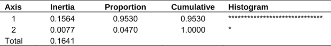
Results of correspondence analysis for year x cane diameter (Cross-tabulation 3) are presented in Table 6. Of total inertia, 95.30% was explained by the first component and 4.70% by the second component (Table 6).
Correspondence Analysis Graph of year × Cane diameter is given in Figure 2. Cane diameter with low level was taken during 2002, one with medium level corresponded to 2006 year. Although year 2005 showed
Eyduran et al. 903
Figure 1. Correspondence Analysis Graph of year × Cane number.
Table 6. Results of correspondence analysis for year × cane diameter.
Axis Inertia Proportion Cumulative Histogram
1 0.1564 0.9530 0.9530 ******************************
2 0.0077 0.0470 1.0000 *
Total 0.1641
equal distance to Cane diameter with high and with medium levels, 2005 year with high level along with year2004 with medium level was similar coordinate area 2003 year had equal distance to low and medium levels.
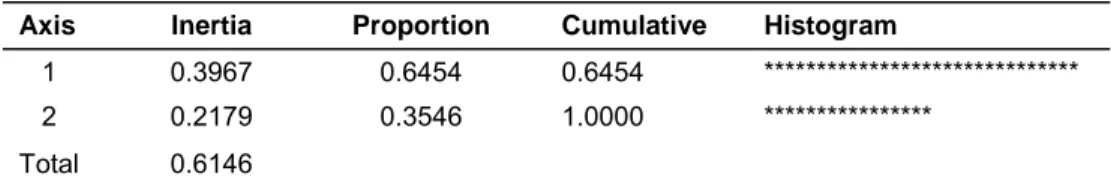
Results of correspondence analysis for Cultivar x cane number (Cross-tabulation 6) are summarized in Table 7. Of total inertia, 64.54% was explained by the first component and 35.46% by the second component (Table 7).
Correspondence Analysis Graph for cultivar × Cane Number is presented in Figure 3. Figure 3 shows that Blacksatin (bsatin) and Jumbo blackberry cultivars had high Cane Number. Ness and Dirkseen Thornless (dthornless) was found to have low cane number. The cultivars having cane number with medium level was Navaho, Chester Thornless, Cherokee and Arapaho
blackberry cultivars.
Results of Correspondence analysis for Cultivar × cane height (Cross-tabulation 7) are given in Table 8. Of total inertia, 93.7% was explained by the first component and 6.30% by the second component (Table 8).
Correspondence Analysis Graph of cultivar × Cane Height is presented in Figure 4. As seen from Figure 4, Arapaho and Cheroke cultivars overlapped each other, and stayed at same distance to high cane height. Ness, Navaho, Black Satin, Dirksen Thornless cultivars also overlapped, and were at equal distance to medium cane height.
As shown in Figure 4, cv. Chester Thornless was closer to high level than medium level, whereas, Jumbo cultivar was closer to medium level than high level.
Figure 2. Correspondence analysis graph of year x cane diameter.
Table 7. Results of correspondence analysis for cultivar × cane number.
Axis Inertia Proportion Cumulative Histogram
1 0.3967 0.6454 0.6454 ******************************
2 0.2179 0.3546 1.0000 ****************
Total 0.6146
Table 8. Results of correspondence analysis for cultivar × cane height.
Axis Inertia Proportion Cumulative Histogram
1 0.8300 0.9370 0.9370 ******************************
2 0.0558 0.0630 1.0000 **
Eyduran et al. 905
Figure 3. Correspondence analysis graph of cultivar × cane number.
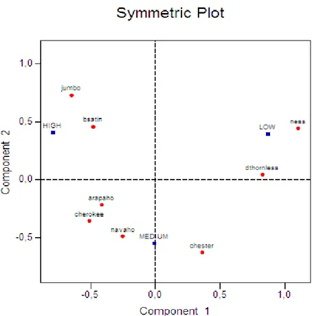
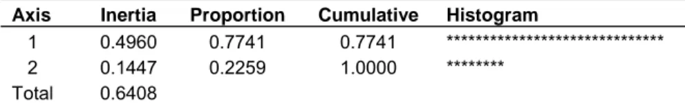
Table 9. Results of correspondence analysis for cultivar x cane diameter.
Axis Inertia Proportion Cumulative Histogram
1 0.4960 0.7741 0.7741 ****************************** 2 0.1447 0.2259 1.0000 ********
Total 0.6408
Figure 5. Correspondence analysis graph of cultivar × cane diameter.
diameter (Cross-tabulation 8) are given in Table 9. Of total inertia, 77.41% was clarified by the first component and 22.59% by the second one (Table 9).
Correspondence Analysis Graph of cultivar × Cane Diameter is presented in Figure 5. As shown in Figure 5, Cheeroke cultivar was determined to have low cane dia-meter. Chester Thornless from blackberry cultivars had high cane diameter. Dirksen Thornless and Black Satin overlapped and was placed exactly between medium and low cane diameter. Jumbo, Ness, and Navaho cultivar were shown to have medium cane diameter. Arapaho
cultivar was roughly between medium and high cane diameter.
Results of Correspondence analysis for Cultivar × cane yield per plant (Cross-tabulation 9) are given in Table 10. Of total inertia, 60% was explained by the first component and 40 % by the second one (Table 10).
Correspondence Analysis Graph of cultivar × Cane yield per plant are presented in Figure 6. According to Figure 6, Chester Thornless cultivar had high cane yield per plant, but Navaho cultivar had medium cane yield per plant.
Eyduran et al. 907
Table 10. Results of correspondence analysis for cultivar × cane yield per plant.
Axis Inertia Proportion Cumulative Histogram
1 1.0000 0.6000 0.6000 ******************************
2 0.6667 0.4000 1.0000 *******************
Total 1.6667
Figure 6. Correspondence analysis graph of cultivar × cane yield per plan.
Other cultivars overlapped, and had low cane yield per plant.
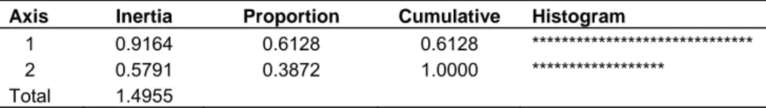
Results of Correspondence analysis for Cultivar × fruit weight (Cross-tabulation 10) are given in Table 11. Of total inertia, 61.28% was explained by the first component and 38.72 % by the second one (Table 11).
Correspondence Analysis Graph of Cultivar × Fruit Weight is presented in Figure 7. It is clear from Figure 7 that Black Satin cultivar had low fruit weight, Arapaho, Navaho, Ness cultivars had medium fruit weight, whereas Chester Thornless and Dirksen Thornless cultivars (which overlapped) were found as high fruit weight as well as Jumbo.
As a result, comparing with chi-square and G statistics, associations between cultivar and each pomological trait (fruit weight, cane number, cane diameter, cane height, and cane yield per plant) were significant (P<0.0001).
The relationship of fruit weight and cane diameter or cane yield per plant was more significant (P<0.0001). The relationship between year and cane number or cane diameter was more significant (P<0.0001).
This is in agreement with Atila et al. (2006a,b); Eyduran et al. (2005a,b); Eyduran and Agaoglu (2006); Siriwoharn et al. (2005); Clark et al. (2005); Yorgey and Finn (2005); Connor et al. (2005a, b); Finn et al. (2005a, b, c, d, e); who reported that genotype, year and genotype by year interaction factors in various studies on blackberry were generally the most crucial factors during selection.
i) Results of the study can be summarized as as high fruit weight was taken in 2004, followed by 2005
ii) Blacksatin and Jumbo blackberry cultivars had the highest cane number.
Table 11. Results of correspondence analysis for cultivar × fruit weight.
Axis Inertia Proportion Cumulative Histogram
1 0.9164 0.6128 0.6128 ******************************
2 0.5791 0.3872 1.0000 ******************
Total 1.4955
Figure 7. Correspondence analysis graph of cultivar × fruit weight.
iii) Arapaho and Cheroke cultivars overlapped each other, and kept the same distance to high cane height.
iv) Chester Thornless blackberry cultivars had the highest cane diameter.
v) Chester Thornless cultivar had the highest cane yield per plant.
vi) Chester Thornless and Dirksen Thornless cultivars had the highest fruit weight.
In view of the above results, cv. Chester Thornless was found as the best blackberry cultivar under conditions of Central Anatolia, Turkey.
REFERENCES
Agresti A (2002). Categorical Data Analysis. 2nd Edn, Wiley, New York. Akturk D, Gun S, Kumuk T (2007). Multiple Correspondence Analysis
Technique Used in Analyzing the Categorical Data in Social Sciences. J. Appl. Sci. 7 (4): 585-588.
Atila SP, Agaoglu YS, Celik M (2006a). A Research on the Adaptation of Some Raspberry Cultivars in Ayaş (Ankara) Conditions. Pakistan J. Biol. Sci. 9(8): 1504-1508.
Atila SP, Agaolu YS, Celik M (2006b). A Research on the Adaptation of Some Blackberry Cultivars in Ayaş (Ankara) Conditions. Pakistan J. Biol. Sci. 9(9):1791-1794.
Baspinar E, Mendes M (2000). İki YOnlü Tablolarda Uyum Analizi Tekniğinin Kullanımı (Usage of Correspondence Analysis Technique
at Contingency Tables) (in Turkish), Ankara Uni. J. Agric. Sci. 6(2): 98-106.
Clark JR, Moore JN, Lopez-Medina J, Finn CE, Perkins-Veazie P (2005). 'Prime-Jan' ('APF-8') and 'Prime-Jim' ('APF-12') primocane-fruiting blackberries. Hortic. Sci. 40: 852-855.
Connor AM, Finn CE, Alspach PA (2005a). Genotypic and environmental variation in antioxidant activity and total phenolic content among blackberry and hybridberry cultivars. J. Am. Soc. Hort. Sci. 130: 527-533.
Connor AM, Finn CE, McGhie TK, Alspach PA (2005b). Genotypic and environmental variation in anthocyaninins and their relationship to antioxidant activity in blackberry and hybridberry cultivars. J. Am. Soc. Hortic. Sci. 130: 680-687.
Duzgunes O, Kesici T, Gürbüz F (1983). Statistics Methods I. University of Ankara, Publishings of Agric. Faculty. Ankara.
Ender P (2005). Applied Categorical & Non-normal Data Analysis Correspondence Analysis.(http://www.gseis.ucla.edu/courses/ed231 c/notes2/corres.html ).
Everitt BS (1992). The Analysis of Contingency Tables. 2nd Edn, Chapman&Hall.London.
Eyduran E, Ozdemir T (2005). Examining Chi-Square, Likelihood Ratio Chi-Square and Independent Ratios in 2x2 Tables: Power of Test. Int. Congress on Info. Technol. Agric., Food and Environ.-itafe’05. Proceedings. Adana-Turkey.
Eyduran E, Ozdemir T, Kucuk M (2005a). Chi-Square and G Test in Animal Science (in Turkish). J. Faculty of Vet. Med. University of Yüzüncü Yıl, pp.1-3.Van-Turkey.
Eyduran E, Ozdemir T, Cak B, Alarslan E (2005b). Using of Logistic Regression in Animal Science, J. Applied Sci., 5(10): 1753-1756. Eyduran E,Ozdemir T, Kara MK, Keskin S, Cak B (2006a). A Study on
Power of Chi-square and G Statistics in Biology Sciences. Pakistan J. Biol. Sci. 9(7): 1324-1327.
Eyduran SP, Agaoglu YS, Eyduran E, Ozdemir T (2006b). Examination of Pomological Features of Different Ten Raspberry Cultivars by the Methods of Various Statistics, Res. J. Agric. Bio. Sci. 2(6): 207-213. Eyduran E, Eyduran SP, Ozdemir T, Agaoglu YS (2006c). Utilization of
Power Analysis in Horticulture, J. Appl. Sci. Res. 2(11): 931-935. Eyduran SP, Agaoglu YS (2006). A Preliminary Examination Regarding
Ten Raspberry Cultivars. Res. J. Agric. Biol. Sci., 2(6): 375-379. Eyduran E, Ozdemir T (2007). Unbiased Estimation for Logistic
Regres-sion. Beykent University, J. Sci. Technol. 1(2):245-251.
Eyduran SP, Agaoglu YS, Eyduran E, Ozdemir T (2007). Comparison of Some Raspberry Cultivars’Herbal Features by Repeated Completed Design Statistic Technique, Pakistan J. Biol. Sci. 10(8): 1270-1275. Finn C, Lawrence FJ, Strik BC (1998). Black Butte trailing blackberry.
Hort. Sci. 32:355-357.
Finn CE, Lawrence FJ, Strik BC, Yorgey B, De Francesco J (1999). ‘Siskiyou’ trailing blackberry. Hortic. Sci. 34: 1288-1290.
Eyduran et al. 909
Finn CE, Yorgey B, Strik BC, Martin RR (2005a). ‘Metolius’ trailing blackberry. Hortic. Sci. 40: 2189-2191.
Finn CE, Yorgey B, Strik BC, Hall HH, Martin RR, Qian MC (2005b). ‘Black Diamond’ trailing thornless blackberry. Hortic. Sci. 40:2175-2178.
Finn CE, Yorgey B, Strik BC, Martin RR, Qian MC (2005c). ‘Black Pearl’ trailing thornless blackberry. Hortic. Sci. 40: 2179-2181.
Finn CE, Yorgey B, Strik BC, Martin RR, Qian MC (2005d). ‘Nightfall’ trailing thornless blackberry. Hort. Sci. 40: 2182-2184.
Finn CE, Yorgey B, Strik BC, Martin RR, Kempler C (2005e). ‘Obsidian’ trailing blackberry. Hort. Sci. 40:2185-2188.
Gauch Jr. HG (1982). Multivariate analysis in community ecology. In: Beck E, Birks, HJ.B & Connor EF (eds) Cambridge studies in ecol. Cambridge University Press, New York 298p.
Keskin S (2001). İki YOnlü (Contingency) Tablolarda Kappa (K) İstatistiğinin Kullanımı, Biyoteknoloji (KÜKEM) Dergisi 25 (1): 53-57. Minitab (2007). Released version 15 (www.minitab.com ).
Ozdemir T, Eyduran E, Keskin S (2006a). Comparison of Chi-Square and Likelihood Ratio Chi-Square Statistics in Social Sciences. Int. Congress on Info. Technol. Agric., Food and Environ.-itafe’05. Proceedings. Adana-Turkey.
Ozdemir T, Keskin S, Cak B (2006b). Calculation of Power in Chi- Square and Likelihood Ratio Chi-Square Statistics by a Special SAS Macro, Pakistan J. Biol. Sci. 9(15): 2798-2801.
SAS (2006). SAS Institute,version 9.0. Inc. Cary, NC, USA.
Siriwoharn T, Wrolstad RE, Finn CE, Pereira CB (2005). Influence of cultivar, maturity and sampling on blackberry (Rubus L. hybrids) anthocyanins, polyphenolics, and antioxidant properties. J. Agric. Food Chem. 52: 8021-8030.
Sokal RR, Rohlf FJ (1996). Biometry. The Principles and Practice of Statistics in Biological Research. W.H. Freeman and Company. New York.
StatSoft Inc (1997). Correspondence Analysis. Electronic Statistics Textbook. Tulsa, WEB: http://sunsite.univie.ac.at/textbooks/statistics/ stcoran.html#general
Strik BC, Clark JR, Finn CE, Bañados MP (2007). Worldwide blackberry production. Hortic. Technol. 17: 205-213.
Strik BC, Mann J, Finn C (1996). Percent drupelet set varies among blackberry genotypes. J. Am. Soc. Hortic. Sci. 121: 371-373.
Yorgey B, Finn CE (2005). Comparison of ‘Marion’ to thornless blackberry genotypes as individually quick frozen and puree products. Hortic. Sci. 40: 513-515.