METHODS FOR AUTOMATIC TARGET
CLASSIFICATION IN RADAR
a thesis
submitted to the department of electrical and
electronics engineering
and the institute of engineering and science
of b
˙Ilkent university
in partial fulfillment of the requirements
for the degree of
master of science
By
Abd¨ulkadir Eryıldırım
July 2009
I certify that I have read this thesis and that in my opinion it is fully adequate, in scope and in quality, as a thesis for the degree of Master of Science.
Prof. Dr. A. Enis C¸ etin (Supervisor)
I certify that I have read this thesis and that in my opinion it is fully adequate, in scope and in quality, as a thesis for the degree of Master of Science.
Assoc. Prof. Dr. U˘gur G¨ud¨ukbay
I certify that I have read this thesis and that in my opinion it is fully adequate, in scope and in quality, as a thesis for the degree of Master of Science.
Asst. Prof. Dr. Sinan Gezici
Approved for the Institute of Engineering and Science:
Prof. Dr. Mehmet Baray Director of the Institute
ABSTRACT
METHODS FOR AUTOMATIC TARGET
CLASSIFICATION IN RADAR
Abd¨ulkadir Eryıldırım
M.S. in Electrical and Electronics Engineering
Supervisor: Prof. Dr. A. Enis C
¸ etin
July 2009
Automatic target recognition (ATR) using radar is an active research area. In this thesis, we develop new automatic radar target classification methods. We focus on two specific problems: (i) Synthetic Aperture Radar (SAR) target clas-sification and (ii)Pulse-doppler radar (PDR) target clasclas-sification. SAR and PDR target classification are extensively used for ground and battlefield surveillance tasks.
In the first part of the thesis, a novel descriptive feature parameter extrac-tion method from Synthetic Aperture Radar (SAR) images is proposed. Feature extraction and classification methods which were developed to handle optical images are usually inappropriate for SAR images because of the multiplicative nature of the severe speckle noise and imaging defects. In addition, SAR images of the same object taken at different aspect angles show great differences, which makes it hard to obtain satisfactory results. Consequently, feature parameter ex-traction method based on two-dimensional cepstrum is proposed and its object recognition results are compared with principal component analysis (PCA) and
independent component analysis (ICA) methods. The extracted feature parame-ters are classified using Support Vector Machines (SVMs). Experimental results are presented.
In the second part of the thesis, the automatic classification experiments over ground surveillance Pulse-doppler radar echo signal are investigated in or-der to overcome the limitations of human operators and improve the classifica-tion accuracy. Covariance method approach is introduced for PDR echo signal classification. To the best our knowledge, the use of covariance method-based classification is not investigated in radar automatic target classification prob-lems. Furthermore, different approaches which involves SVMs are developed. As feature parameters, cepstrum and MFCCs are used. Performances of these two approaches are compared with the Gaussian Mixture Models (GMM) based classification scheme. Experimental results and conclusions are presented.
Keywords: Target classification, radar, feature extraction, principal component
analysis, independent component analysis, Support Vector Machine, Gaussian Mixture Models, region covariance, covariance matrix
¨
OZET
RADARDA HEDEF SINIFLANDIRMA ˙IC
¸ ˙IN Y ¨
ONTEMLER
Abd¨ulkadir Eryıldırım
Elektrik ve Elektronik M¨uhendisli¯gi B¨ol¨um¨u Y¨uksek Lisans
Tez Y¨oneticisi: Prof. Dr. A. Enis C
¸ etin
Temmuz 2009
Radar kullanarak otomatik hedef tanıma, etkin bir ara¸stırma alanıdır. Bu tezde, radar sistemler i¸cin otomatik hedef sınıflandırma y¨ontemleri geli¸stirilmi¸stir. ˙Iki belirli problem ¨uzerinde durulmu¸stur: (i) Her t¨url¨u hava ko¸sulunda g¨or¨unt¨uleme sa˘glayan, Sentetik Diyafram Radar (SAR) hedef sınıflandırılması (ii) Pulse-Doppler (PDR) hedef sınıflandırılması.
Tezin birinci b¨ol¨um¨unde, SAR g¨or¨unt¨ulerinden yeni bir betimleyici ¨oznitelik ¸cıkarma y¨ontemi ¨onerilmektedir. Yo˘gun ¸carpımsal benek g¨ur¨ult¨u ve g¨or¨unt¨uleme hatalarından dolayı, optik imgeler i¸cin geli¸stirilen ¨oznitelik ¸cıkarma ve sınıflandırma y¨ontemleri, SAR g¨or¨unt¨uleri i¸cin genellikle uygun olmamak-tadır. Bunun yanısıra, aynı nesnenin farklı a¸cılardan elde edilen SAR g¨or¨unt¨ulerinin b¨uy¨uk farklılıklar g¨ostermesi, tatmin edici sonu¸clar elde edilmesini zorla¸stırmaktadır. Sonu¸c olarak, iki boyutlu ‘cepstrum’u temel alan bir ¨oznitelik ¸cıkarma parametresi ger¸cekle¸stirilmi¸s ve nesne sınıflandırma performansı temel bile¸sen analizi ve ba˘gımsız bile¸sen analizi y¨ontemleri ile kar¸sıla¸stırılmı¸stır. C¸ ıkarılan ¨oznitelikler Dayanak Vekt¨or Makinaları kullanılarak sınıflandırılmı¸stır. Deneysel sonu¸clar sunulmu¸stur.
Tezin ikinci b¨ol¨um¨unde ise, insan operat¨orlerinin dezavantajlarını gider-mek ve sınıflandırma do˘grulu˘gunu artırmak i¸cin, kara g¨ozetleme amacıyla kul-lanılan Darbe Doppler radar yankı sinyali ¨uzerinde otomatik sınıflandırma deneyleri ger¸cekle¸stirilmi¸stir. Ortak de˘gi¸sinti tabanlı sınıflandırma sunulmu¸stur. Bildi˘gimiz kadarıyla, ortak de˘gi¸sinti kullanarak sınıflandırma yapma yakla¸sımı, radar otomatik hedef sınıflandırma problemlerinde incelenmemi¸stir. Bunun yanısıra, SVM i¸ceren farklı yakla¸sımlar geli¸stirilmi¸stir. ¨Oznitelik parametreleri olarak, ‘cepstrum’ ve ‘MFCC’ katsayilari kullanilmi¸stir. ¨Onerilen iki y¨ontemin performansları, Gauss Karı¸sım Modelleri (GMM) tabanlı sınıflandırma y¨ontemi ile kar¸sıla¸stırılmı¸stır. Deneysel sonu¸clar sunulmu¸stur.
Anahtar Kelimeler: Hedef sınıflandırma, radar, ¨oznitelik ¸cıkarma, temel bile¸sen
analizi, ba˘gımsız bile¸sen analizi, Dayanak Vekt¨or Makinaları, Gauss Karı¸sım Modelleri, b¨olgesel de˘gi¸sinti, de˘gi¸sinti matrisi
ACKNOWLEDGMENTS
I was so lucky and proud to have Prof. Dr. A. Enis Cetin as my advisor. I would like to express my thanks and gratitude to my advisor for his supervision, guide and invaluable encouragement during my graduate study and the development of this thesis. His wisdom in solving problems and generating ideas helped me to improve my research capabilities and enhanced my vision.
Also I would like to thank Asst. Prof. Dr. Sinan Gezici and Asst. Prof. Dr. U˘gur G¨ud¨ukbay for agreeing to serve on my thesis committee. I would also like to thank T ¨UB˙ITAK for its financial support. I would like to thank my colleagues in METEKSAN SAVUNMA A.S¸. for their support and encouragement during my graduate study.
I also extend my special thanks to Suat Bayram, Aykut Yıldız, Mehmet Burak G¨uldo˘gan, Mahmut Yavuzer, Bahaddin Eravcı, Canay ¨Ozkan, Ahmet ¨Ozdemir, Mustafa ˙Incebacak for being wonderful friends and sharing unforgettable mo-ments together.
Finally, I would like to say thanks to my mother, Fatma, and my father, Mustafa, and my brothers, Ibrahim and Burak, for their unconditional love and support throughout my life and studies. My deepest gratitude goes to my love, Derya, for her support and love which have been invaluable in helping me focus on my academic pursuits.
Contents
1 Introduction 1
1.1 Objectives and Contributions of the Thesis . . . 1
1.2 Statistical Pattern Recognition Model for Automatic Target Clas-sification in Radar . . . 5
1.3 Organization of the Thesis . . . 7
2 Automatic Target Classification for High-Resolution Synthetic Aperture Radar (SAR) 9 2.1 Syntetic Aperture Radar Image Formation and Properties . . . . 10
2.2 Principal Component Analysis . . . 13
2.3 Independent Component Analysis . . . 14
2.4 2-D Cepstrum Based Feature Extraction . . . 14
2.5 MSTAR Database . . . 18
2.6 Experimental Results Over MSTAR Database and Discussions . . 20
2.6.2 Target Classification . . . 23
3 Automatic Target Classification for Surveillance Pulse-Doppler Radar 27 3.1 Cepstral Analysis . . . 28
3.1.1 1-D Cepstrum . . . 28
3.1.2 Mel-Frequency Cepstrum Coefficients (MFCC) . . . 28
3.2 Covariance-based Classification Approach . . . 30
3.3 Support Vector Machine Based Classification Approach . . . 32
3.3.1 Training of the First Stage SVMs . . . 33
3.3.2 Training of the Second Stage SVMs . . . 33
3.3.3 Testing of the First Stage SVMs . . . 34
3.3.4 Testing of the Second Stage SVMs . . . 35
3.4 Experimental Results and Discussion . . . 35
3.4.1 Database Description . . . 35
3.4.2 Target Classification Experiments . . . 37
4 Conclusions 50
Bibliography 53
A Support Vector Machines 57
B Gaussian Mixture Models 59
B.0.3 Maximum Likelihood Parameter Estimation . . . 60
List of Figures
1.1 Statistical Target Classification Model . . . 7
2.1 Illustration of SAR geometry and data collection scheme (Cour-tesy of Sandia National Laboratories.) . . . 12
2.2 Representation of a sample non-uniform grid (for 128 by 128 im-ages) for 2-D Cepstrum computation . . . 16
2.3 A sample MSTAR target (BMP-2 vehicle) image (128 by 128) and its cepstral image . . . 17
2.4 2-D Cepstrum method block diagram . . . 18
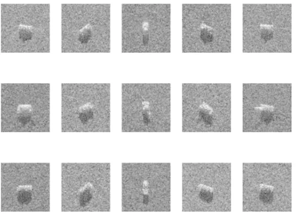
2.5 MSTAR target images with different orientations (aspect angles), BMP-2, T-72 and BTR-70, correspondingly from top row to bot-tom row . . . 19
2.6 SAR image of the MSTAR target array (left) at Redstone Arse-nal in Huntsville, Alabama, and with ground truth superimposed (right). The radar illumination is from the top (Obtained from MIT Lincoln Laboratory) . . . 20
2.8 Performance Comparison of the Methods for original SAR images
of size 128x128 . . . 23
3.1 Mel-scale feature extraction . . . 28
3.2 Filters for computing mel-frequency cepstrum co-efficients . . . . 30
3.3 Two stage SVM classification scheme . . . 32
3.4 Spectrogram of wheeled vehicle . . . 36
3.5 Spectrogram of tracked vehicle . . . 37
3.6 Spectrogram of clutter . . . 38
3.7 Spectrogram of one person . . . 39
3.8 Spectrogram of two persons . . . 40
3.9 Radar echo samples of wheeled vehicle . . . 41
3.10 Radar echo samples of tracked vehicle . . . 42
3.11 Radar echo samples of one person . . . 43
3.12 Radar echo samples of two persons . . . 44
3.13 Radar echo samples of clutter . . . 45
3.14 Classification accuracy of the GMM method using cepstrum and MFCC features for the five-class problem as function of number of features (Frame length is 4 seconds and model order is 10 for all classes) . . . 46
3.15 Classification accuracy of the GMM method using cepstrum and MFCC features for the five-class problem as function of frame length (Number of features and Gaussian components is 10) . . . 47
3.16 Classification accuracy of the GMM, covariance and SVM based methods using cepstrum features for the five-class problem as func-tion of frame length (Model order is 12 for GMM-based approach for all classes and number of features is 10 for all methods) . . . . 48
3.17 Classification accuracy of the GMM, covariance and SVM based methods using cepstrum features for the five-class problem as func-tion of number of features (Model order is 12 for GMM-based approach for all classes) . . . 49
A.1 The Visualization of the SVM classification scheme. C0 is the op-timal hyper-plane because it maximizes the margin - the distance between the hyper-planes H1 and H2. . . 57
Chapter 1
Introduction
1.1
Objectives and Contributions of the Thesis
Automatic target recognition (ATR) using radar is an active research area [1]. With the advances in computer technology, real time target classification and recognition becomes an important and essential feature (function) of radar sys-tems, specifically for military purposes [2]. Radar sensor information to locate, track and identify oppositional forces provides several tactical benefits and su-periority for military forces.
In this thesis, we develop new automatic radar target classification methods. We focus on two specific problems : (i) Synthetic Aperture Radar (SAR) tar-get classification, which allows to monitor the areas in all-weather conditions and (ii)Pulse-doppler radar (PDR) target classification. SAR and PDR target classification are extensively used for ground and battlefield surveillance tasks.
A typical and complete SAR automatic target recognition (ATR) system includes five stages: detection, discrimination, classification, recognition, and
identification [3]. In some systems, only some of the above stages are avail-able. Sometimes, the three terms, classification, recognition and identification may refer to the same meaning. In Chapter 2, we investigate SAR target clas-sification/recognition and introduce our novel feature extraction method, which is based on two-dimensional (2-D) cepstrum. Target classification/recognition includes discriminating target signatures from the ones coming from the clutter (buildings,trees, farms etc) and non-target objects (confuser vehicles etc) as well as recognizing targets by type within a class [3]. Automatic recognition and clas-sification of man-made objects in Synthetic Aperture Radar (SAR) images have gained great importance and interest because the hardware and quality of SAR systems has improved dramatically in the last two decades. Furthermore, SAR sensors can produce images of the scenes in all weather conditions at any time of day and night that are not possible with infrared or optical sensors [1]. There are many areas of application where the recognition of a target or texture in SAR images is important including military combat identification, meteorological ob-servation, battlefield surveillance, mining and oceanography [4]. Considering the emergence and proliferation of low-cost, high-resolution sensor platforms, specif-ically on Unmanned Air Vehicles (UAVs), and the current trend, SAR systems will probably be ubiquitous, operating on many different types of platforms and tasks in the near future. This leads to a huge increase in the amount of collected SAR data and need in efficient, powerful and state of the art methods in order to extract valuable information from them. SAR sensors promise great potentials in military battlefield operations by detecting and classifying military targets remotely in all weather-conditions providing a great tactical advantage [2].
Feature extraction and classification methods which have been developed to handle optical images are usually inappropriate for SAR images [4]. Feature-based approaches are naturally suited for optical images. For instance, when an object in an optical image has visible tracks and a gun-barrel, it is a tank or simi-lar vehicle. However, this approach fails for SAR imagery since SAR images may
not reflect true features of the target due to imaging defects, geometric distor-tions and severe speckle noise. Understanding and interpreting basic properties of of SAR images is necessary for effective use of SAR data. For instance, SAR images of the same target taken at different aspect angles show great differences, which makes it hard to obtain satisfactory results. Occlusions and illumination changes may yield dramatic differences from image to image taken with differ-ent angles. In order to deal with these problems, domain-specific and efficidiffer-ent methods should be developed.
In the simplest approach, object classification could be done based on pattern-matching techniques using whole available information in the data. However, this approach is time consuming and computationally costly. Furthermore, since SAR images contain enormous number of pixels, it is needed to reduce the di-mensionality of data before the classification stage. Statistical feature extraction and classification methods have been applied to SAR target classification. In the state of the art works, Support Vector Machines (SVMs) are extensively used and they promise high recognition performances since they have several advantages over traditional classifiers such as neural networks [5]. A number of approaches describing the use of Support Vector Machines (SVMs) can be found in [6] - [7]. In [7], it is stated that SVMs present better results than conventional classifiers in SAR target recognition.
Several approaches applied to SAR ATR were examined in [8] with a com-plexity consideration. Topographic features are used in automatic classification of targets in SAR imagery in [9]. Targets are classified using a Topographi-cal Primal Sketch that assigns each pixel a label that absorbs monotonic grey tone transformations. In [10], a new model for SAR ATR that incorporates the estimation of target pose is presented.
Among the statistical approaches, it has been claimed that principal com-ponent analysis and independent comcom-ponents analysis provide discrimination of
SAR military targets when used with a SVM classifier [11]. Image moments, which are used in optical images as shape descriptors, usually fail in SAR clas-sification systems since shapes of targets in SAR images are geometrically dis-torted versions of true target shapes and they are severely affected by speckle noise and Signal-to-Noise Ratio (SNR) of the SAR system [12]. Wavelet-based feature extraction schemes were also used to represent accurate classification on the MSTAR public domain database images. In [13], wavelet transforms along with SVM classifier were used.
In [14], Elliptical Fourier Descriptors and SVMs are used in achieving a SAR ATR task. This work is related to our novel 2-D cepstrum method, presented and investigated in Chapter 2 of this thesis, in the sense that Fourier transforms are utilized to extract features.
In Chapter 3, we investigate the automatic classification experiments over ground surveillance Pulse-doppler radar echo signal in order to overcome the limitations of human operators. Furthermore, covariance method approach is introduced for PDR echo signal classification [15]. To the best our knowledge, the use of covariance method-based feature extraction is not investigated in radar automatic target classification problems.
Detection and classification of ground moving and stationary targets are of the main functions of ground surveillance radars. Typically, target detection is done automatically, however, human operators also take an essential part in the target classification. By listening to the audio tone of the target, which is a representation of the target’s Doppler frequencies, trained operators can classify a target with a reasonable degree of accuracy. However, this audio-based human classification scheme suffers from some short-comings. First of all, the classification tasks keep the operator busy and he or she may stop the execution of other radar functions in a proper manner, i.e., this approach increases the load of work which should be handled by the radar operator, such as listening
carefully to the audio, focusing on the target of interest etc. Finally, training of operators is necessary and needs allocation of time and other valuable resources. An automatic classification system is an important improvement and valuable support for ground surveillance systems.
In [16], preliminary results of radar target recognition using speech recog-nition based methods are reported. In [17], Doppler-signature based features along with Hidden Markov Models (HMM)- Gaussian Mixture Models (GMM) based classification provide 88% recognition rate. However, Doppler signatures perform worse for small changes in aspect angle. Besides that, in this work, it is claimed that neural network classifier perform much worse than HMM-GMM based classifier. A similar result is achieved by [17], in which conditions of spec-trum stationarity is pointed out.
We adapt cepstrum and Mel-Frequency Cepstrum Coefficients (MFCCs) as features and GMM as classifier, which are extensively used in speech recognition, in order to obtain superior performance results in case of radar target classifi-cation. Furthermore, we propose the use of region covariance approach, which is used in object detection in still images and videos in [15], in classifying the targets from the echo signals. We show that covariance based approach pro-vides superior classification accuracies and computationally efficient. Moreover, different approaches which involves SVMs are developed.
1.2
Statistical Pattern Recognition Model for
Automatic Target Classification in Radar
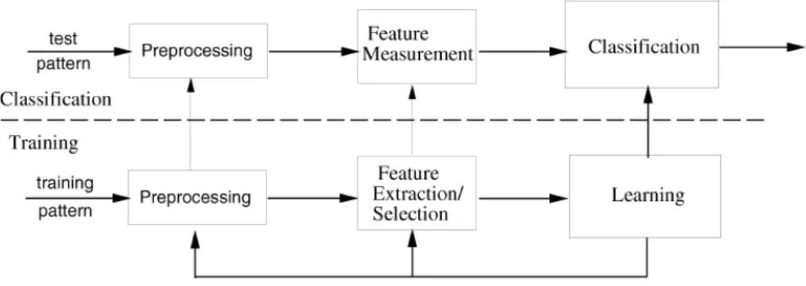
The statistical pattern recognition model we use for Radar automatic target classification in this thesis is illustrated in Figure 1.1. This model is general basis for our classification approach and system designs.
In statistical pattern recognition, features are extracted from patterns which characterize an observation, which may be a SAR image or a speech signal. A set of d features constitutes a d-dimensional feature vector and obtaining feature parameters from signal patterns is called feature extraction. Usually, the dimensionality of feature space is smaller. After obtaining features [18], in order to determine decision boundaries in the feature space between pattern classes, methods from statistical decision theory are used. The decision boundaries are established by the probability distributions of the patterns corresponding to each class, which is either specified or learned. For example, the direct boundary construction approaches which are supported by Vapnik’s philosophy [6] lead to Support Vector Machines, which are superior to many existing classifiers in many practical applications.
The purpose of the pre-processing stage is to isolate the interested pattern from the background or clutter, to denoise and other operation which can be feasible in obtaining a good representation of the pattern.
Classification is categorized into two types : supervised and unsupervised classification. In supervised classification approach, classes are defined by the system designer. Therefore, the input pattern is a member of pre-defined class. However, in unsupervised classification scheme, the classes are determined using the similarity of classes and the input pattern is assigned accordingly. In our cases, targets are known a priori and thus, supervised approaches are considered.
Supervised pattern recognition systems have two modes: training (learning) and classification (testing). In the training mode, the feature extraction/selection module constructs the features which are representations of the input pattern and then the classifier is trained in order to segment the feature space, i.e., to determine the decision boundaries in the feature space. The feedback in the model is used to adjust the preprocessing and feature extraction methods if needed. In the classification (testing) mode, the trained classifier determines
the class of the input pattern using the measured features. Figure 1.1 shows these stages and operation modes. There exists no single optimal classification
Figure 1.1: Statistical Target Classification Model
approach or method. Therefore, multiple approaches and methods should be utilized. Every problem should be handled in its domain and circumstances in order to take advantage of the specific nature of the problem.
Feature extraction depends on the characteristics of the input pattern. The stages in Figure 1.1 should be combined and optimized altogether to obtain the optimal solution. However, this may not be possible in many practical applica-tions.
1.3
Organization of the Thesis
The organization of the thesis is as follows. In Chapter 2, SAR automatic target classification/recognition problem is investigated and a novel feature parameter extraction method, which is based on 2-D cepstrum, is introduced. This novel 2-D cepstrum method is compared with principal component analysis (PCA) method and independent component analysis (ICA) by testing over the MSTAR image database. The extracted features are classified using the Support Vec-tor Machine (SVM). We demonstrate that discrimination of natural background
(clutter) and man-made objects (metal objects) as well as recognition of military targets in SAR imagery is possible using the 2-D cepstrum feature parameters. Also, it is shown that 2-D cepstrum approach provides better classification ac-curacies. Experimental results are presented. In Chapter 3, the automatic clas-sification experiments over ground surveillance Pulse-doppler radar echo signal is performed in order to overcome the limitations of human operators. Three different approaches, which involve Gaussian Mixture Models, covariance ma-trix and SVMs, are presented and their performances are compared by doing several experiments. To the best of our knowledge, covariance based approach is not investigated in radar target classification. Cepstral features, which in-clude cepstrum and MFCC parameters, are used in the experiments and studies. Experimental results are presented. Finally, Chapter 4 concludes the thesis.
Chapter 2
Automatic Target Classification
for High-Resolution Synthetic
Aperture Radar (SAR)
This chapter is organized as follows. In Section 2.1, SAR imaging process and properties of SAR images are explained briefly. In Section 2.2, Principal Com-ponent Analysis (PCA) based SAR ATR, is described and in Section 2.3, In-dependent Component Analysis (ICA) based method is explained. In Section 2.4, our novel feature extraction method, which is based on 2-D cepstrum, is introduced and presented. In Section 2.5, MSTAR SAR image database is re-viewed. Experimental classification results obtained by applying 2-D cepstrum based proposed method, principal component analysis (PCA) and independent component analysis (ICA) are presented over the MSTAR database in Section 2.6.
2.1
Syntetic Aperture Radar Image Formation
and Properties
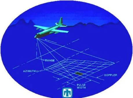
Synthetic Aperture Radar is a remote sensing device used in moving aerial ve-hicles and it produces high resolution images of scenes in both range and in cross-range (a direction parallel to the vehicle motion) by synthesizing the effect of a large antenna aperture based on signal processing. Motion of the radar, which corresponds to phase shifts (can be regarded as Doppler frequencies) in received signals, is exploited properly to obtain a two-dimensional representa-tion of the scene. Each pulse, emitted by the radar, reaches to the target area where the antenna beam intercepts the ground and illuminates the targets lo-cated there, and the reflected return pulses are in turn collected by the same antenna along sensor path during motion, as shown in Figure 2.1.
SAR is most widely used radar system for monitoring of the earth surface and imaging of stationary targets on the ground. The imaging capability of SAR can be utilized for military reconnaissance, measurement of earth surface conditions, geological mapping, classification of terrain, mineral explorations and other remote sensing application. The wide application range of SAR led to the development of great number of airborne and space-borne SAR systems.
Figure 2.1 shows the configuration and geometry of a typical SAR system. The SAR image formation algorithms produce an image of the scene in slant range and azimuth coordinates. Detailed description of the theory of SAR imag-ing is beyond the scope of this thesis. The purpose of this section is to give a brief introduction about essential properties of SAR images, how SAR works and operates to generate SAR images.
Essentially, SAR data provides measurements of the complex radar reflectiv-ity of the scene. Basically, a SAR image is a result of turning this two-dimensional
set of measurements into information about the scene. These measurements made by the SAR are fundamentally determined by electromagnetic scattering processes.
For a point-target case (point-scatterer) and single channel SAR, Equa-tion (2.1) theoretically defines the most general descripEqua-tion of SAR scattering process, the complex reflectivity Spq and its relation between polarization state
of p of an incident plane wave with polarization q under reasonable assumptions [4]. R is the slant range of the scatterer in far-field. The incident electric field has complex components represented by Ei
p and Eqi and the scattered field has
components given by Es p and Eps: Eps Es q = e2πiR/λ R Spp Spq Sqp Sqq Epi Ei q (2.1)
The 2X2 matrix on the right-hand side of Equation (2.1) is defined as the scattering matrix (for further information see [4]). For SAR systems, radiometry and phase preservation are a critical issue. The scattering mechanism is the main phenomenon behind the multiplicative speckle noise in SAR images. With only accurate estimates and reasonable system performance, target information extracted from SAR images can be regarded as meaningful. The SAR system can modify and distort the properties of a target and produce artifacts caused by errors and defects in the system behavior and the signal processing system.
The advantages of SAR systems and the reasons why SAR is used as an essential remote sensing device can be expressed as follows:
• SAR is an active sensor that uses its own illumination (it emits its own
electromagnetic wave).
• SAR operates in all weather conditions (cloudy, rainy, snowy, etc.), day
• Depending on the frequency band employed, SAR systems provide
pene-tration into the cloud, soil of ground surface or ice.
• Theoretically, resolution is independent of the distance to the target. • The scattering process of SAR systems demonstrates different properties
than visible light and provides information about the scene or the target, depending on operating frequency.
Figure 2.1: Illustration of SAR geometry and data collection scheme (Courtesy of Sandia National Laboratories.)
Unlike optical images, the SAR image of a target reflects the structure of point scatterers of the target, which is determined by the reflectivity of the target, radar geometry (illumination) and electromagnetic scattering process. Thus, SAR images of the same target obtained at different aspect angles exhibit great differences, which in turn makes classification task harder. Occlusions in parts of the target happen due to illumination by the radar from a certain pose. Therefore, orientation of the target and radar with respect to each other results in great differences in SAR images of the same target, which can be observed
2.2
Principal Component Analysis
Principal Component Analysis (PCA) is one of the most popular methods used in feature extraction in SAR images [7]. PCA can reveal patterns, similarities and differences in data and it is a powerful data analysis approach. PCA method can be used to compress the data by concentrating on significant (principal) components of the data with a tolerable loss of information.
The PCA method projects d dimensional data x onto a lower-dimensional subspace by minimizing the sum-squared error [8]. The first step of the PCA is the computation of the d-dimensional mean vector µ and d by d covariance matrix Σ using the full dataset (i.e., the training dataset). Next, the eigenvectors and eigenvalues are computed and eigenvectors are ordered according to the decreasing eigenvalue. This provides the components in order of significance. Then, p eigenvectors having the largest eigenvalues are selected and a d by p matrix T whose columns are the the p eigenvectors is constructed. The feature vector of the input data ˜x is extracted by projecting the input data x onto the p-dimensional subspace using the equation:
˜
x = Tt(x − µ) (2.2)
where Tt is the transpose of the matrix T.
In conclusion, principal component analysis yields a p-dimensional linear sub-space of feature sub-space that best represents the full data according to a minimum-square criterion. PCA method is widely applied in many types of signal anal-ysis in neuroscience, face recognition and image compression due to its simple, non-parametric nature and ability to reduce high dimensional data to a lower dimension.
2.3
Independent Component Analysis
While principal component analysis try to find directions in feature space that best represent the data in a sum-squared error sense, independent component analysis (ICA) seeks directions that are most independent from each other and it can be seen as blind source separation. Thus, ICA is a method used to separate linearly mixed sources [18]. ICA tries to solve the problem of how the observed data x can be represented as a superposition of independent components sj’s,
which is given by:
x = As (2.3)
where x is the observed vector that includes the observations xj’s, s is the
source vector that consists of the independent components si’s and A is the
mixing matrix.
In ICA, vector x is the only a priori known parameter and both A and s are assumed to be unknown. Therefore, A and s should be estimated under the assumption that s is non-Gaussian and entries of the s vector are statistically independent [19].
Once A is estimated, ICA computes the sources by exploiting the given as-sumptions in the model to estimate both A and s using the following equation:
s = W x, (2.4)
where W is (the demixing matrix) the (pseudo)inverse of the mixing matrix A
2.4
2-D Cepstrum Based Feature Extraction
In this section, we present the 2-D cepstrum approach to extract descriptive features from SAR images. The real cepstrum of ˆx(n1, n2) of a 2-D signal x is
defined as:
ˆ
x(n1, n2) = F2−1(log(|X(u, v)|)) (2.5)
where (n1,n2) are the 2-D cepstrum domain coordinates, F2−1represents the 2-D
inverse discrete-time Fourier transform (IDTFT) and X(u, v) is the discrete-time Fourier transform (DTFT) of the original signal x. In Equation (2.5), the DTFT and IDTFT are computed using the FFT algorithm on a uniform grid. However, a non-uniform grid is used in IDFT in this paper similar to the mel-cepstrum used in speech recognition. This is because object edges are not strong in SAR images and SAR images are heavily corrupted by inherent high-frequency speckle noise. Therefore, low frequency bands should be emphasized as in speech processing. Our 2-D cepstrum feature method applied to 2-D SAR images comprises of four major steps:
1. Compute the magnitude of the 2-D discrete-time Fourier transform (DTFT) of the SAR image region.
2. Transform the 2-D DTFT data into non-uniform 2-D DTFT grid and apply weights to sub-bands
3. Compute log(|X(u, v)|)
4. Apply inverse 2-D discrete-time Fourier transform (IDTFT) to obtain ˆx
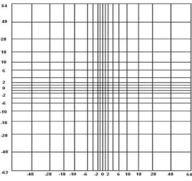
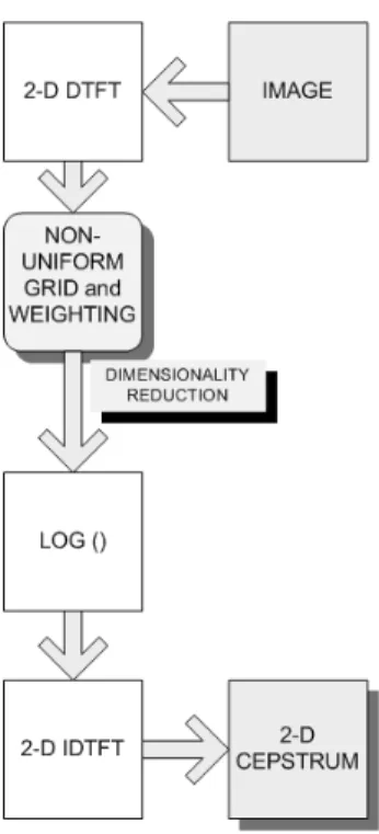
Figure 2.4 illustrates the process of computing the 2-D cepstrum feature param-eters of a given SAR image. The 2-D DTFT grid is non-uniformly divided into cells varying in size and the weighted mean or variance value of each cell is used in the proposed algorithm. Weights are assigned higher values to low frequency bands. In this way, low frequency bands containing most of the target energy is emphasized compared to high frequency bands. Since speckle noise affects the high frequency components, this stage also plays the role of a de-noising process.
Figure 2.2: Representation of a sample non-uniform grid (for 128 by 128 images) for 2-D Cepstrum computation
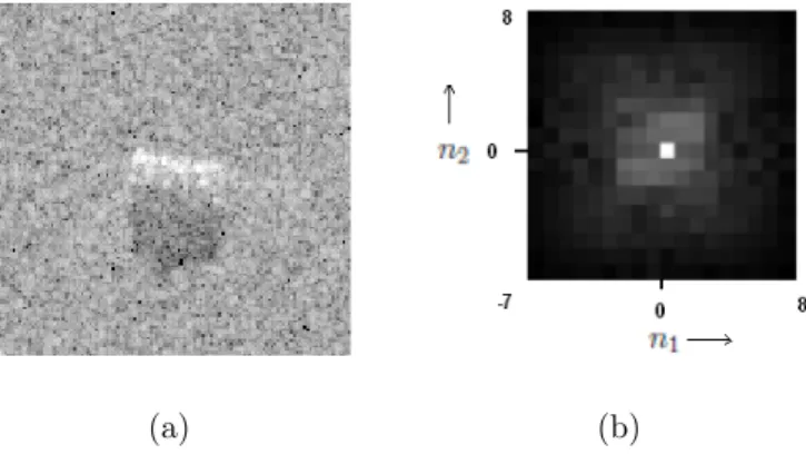
A non-uniform sample grid is shown in Figure 2.2. The N by N 2-D DTFT matrix is reduced to L by L (L ≤ N) matrix by use of a non-uniform grid. To reduce the computational cost, L can be selected as a power of 2. In Figure 2.3, a sample SAR image of a target (BMP-2) and the final result of cepstral processing of this image are shown. The size of cepstrum matrix is much smaller than the size of the original target image. Furthermore, since SAR images are real images, only one half of 2-D cepstrum is sufficient to represent the target image due to the properties of Fourier transform. The proposed 2-D cepstrum based feature extraction provides dimensionality reduction, which enables to represent the tar-get with reduced complexity. Moreover, one of the most important properties of cepstrum is shift-invariance. Assume that y(n1, n2) = x(n1− k, n2− l). Then,
the real cepstrum of y can be expressed as: ˆ
y(n1, n2) = F2−1(log(|Y (u, v)|)) (2.6)
ˆ
y(n1, n2) = F2−1(log(|X(u, v)e−2πj(uk+vl)|)) (2.7)
ˆ
(a) (b)
Figure 2.3: A sample MSTAR target (BMP-2 vehicle) image (128 by 128) and its cepstral image
Consequently, it is obtained that:
ˆ
y(n1, n2) = ˆx(n1, n2) (2.9)
Therefore, cepstral parameters are not affected by the location of the target in the SAR image. The contents of the 2-D cepstrum matrix can be used to form a feature vector.
Furthermore, discrete cosine transform (DCT) can be used instead of the Fourier transform to reduce the computational load. We tried this method and obtained satisfactory results as the Fourier transform. Consequently, for compu-tational considerations, it is reasonable to use DCT instead of FFT. Therefore, in our implementations, we used DCT for faster processing. One of the princi-pal benefits of the log transformation in the cepstral processing is to compress dynamic range and it provides invariance to the scale changes in amplitude and rotational variations to some extent. Let X be the 2-D image of an object and
aX is its amplified (or attenuated) version. The log spectrum of the aX is given
Figure 2.4: 2-D Cepstrum method block diagram ˆ xa(n1, n2) = ˆaδ(n1, n2) + ˆx(n1, n2) where δ(n1, n2) = 1 , when n1 = 0, n2 = 0 0 , otherwise . (2.10)
Therefore, the amplitude parameter a only effects the (0, 0)th entry (DC level) of the centered 2D cepstrum. Therefore, cepstral parameters except the (0, 0)th entry are invariant to amplitude variations of the original image. This is a very important feature of the cepstrum because the signal strength and quality of the 2-D SAR image may get affected by the look-angle change and the speckle noise.
2.5
MSTAR Database
In this work, MSTAR SAR image database is used. MSTAR is the abbrevia-tion of the Moving and Staabbrevia-tionary Target Acquisiabbrevia-tion and Recogniabbrevia-tion program which is a joint Defense Advanced Research Projects Agency (DARPA) and Air
Force Research Laboratory (AFRL) effort. The data includes a series of 1 foot by 1 foot (0.3-m by 0.3-m) resolution spot-light mode SAR images which were collected using the Sandia National Laboratories Twin Otter SAR sensor pay-load operating at X band. Each target was imaged at various depression angles. The standard chip size per target type is 128 by 128. Each image is associated width a separate file. The files have a header that contain information about the target parameters including: target model number; type of vehicle (tank, trans-port, truck, etc.); serial number of the target; pose (Azimuth Heading); pitch; roll; yaw; depression angle; radar ground squint angle; range; and several other parameters.
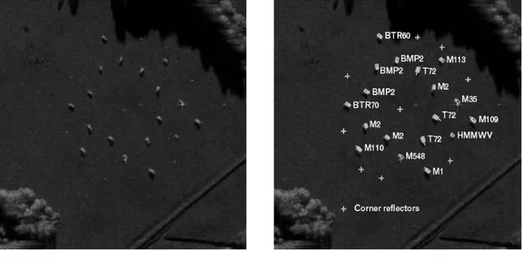
The targets which refer to man-made (metal) objects in this paper are BMP-2, BTR-70 armored personal carriers and T-72 main battle tank. The clutter refers to the natural background and man-made objects other than the targets. Figure 2.6 shows a typical MSTAR SAR spotlight image (0.3-m x 0.3-m
res-Figure 2.5: MSTAR target images with different orientations (aspect angles), BMP-2, T-72 and BTR-70, correspondingly from top row to bottom row
Figure 2.6: SAR image of the MSTAR target array (left) at Redstone Arsenal in Huntsville, Alabama, and with ground truth superimposed (right). The radar illumination is from the top (Obtained from MIT Lincoln Laboratory)
2.6
Experimental Results Over MSTAR Database
and Discussions
2.6.1
Target Detection Using 2-D Cepstral Features
In this work, we try to discriminate the targets which refer to man-made (metal) objects, BMP-2, BTR-70 armored personal carriers and T-72 main battle tank, from the clutter which refers to the natural background and other man-made objects. Figure 2.7 shows some MSTAR sample images used in our experiments. In general, given a SAR image, region of interests (ROIs) are determined using a constant-false alarm rate (CFAR) method [4]. In this way, first, possible tar-get areas are detected and then ROIs are classified using an object recognition method. The target region of interests (ROIs), which are of size 128 by 128, are available in the MSTAR database and clutter ROIs with the same size are generated from the original images in the MSTAR database by cropping. In this experimental study, no filter is implemented to reduce the speckle noise in SAR
Figure 2.7: MSTAR target and clutter image examples
images. Examples of target and clutter ROI images (which are 128 by 128) are shown in Figure 6. We used 128 by 128 ROI images and also 96 by 96 image chips obtained from the ROI images by cropping the target area, usually located in the center of the 128 by 128 ROI images.
Training and test sets with two classes containing targets and clutter (no target) are constructed. Number of samples corresponding to each category is shown Table 2.1. The 2-D cepstral feature parameters are computed from each input ROI and they are classified using Support Vector Machines (SVM). Publicly available LIBSVM software [20] is used. Principal Component Analysis (PCA) and Independent Component Analysis are also implemented to obtain the feature vectors from SAR images to compare the performance of the proposed cepstral domain feature extraction method.
Table 2.1: Number of images used in experiments Number of training samples Number of test samples
Target 1376 1376
Clutter 1307 11007
We define the detection accuracy of each method as the number of correctly detected targets divided by the total number of sample images tested. The false alarm percentage (PF) is equal to the number of false positives (clutter samples
Table 2.2: Target detection in MSTAR database
Input Images Performance Measures 2-D Cepstrum PCA ICA
128 by 128 Detection Acc.(%) 99.29 98.64 95.65
PF (%) 00.10 00.15 00.72
96 by 96 Detection Acc.(%) 99.71 99.45 95.72
PF (%) 00.03 00.04 00.64
which are misclassified) divided by the total number of sample images tested. The target detection results are summarized in Table 2.2.
The best classification results are obtained using the 2-D cepstral feature parameters which are classified using the radial basis function (RBF) kernel of the SVM. The 2-D feature parameters are obtained from a 6 by 6 region in cepstral domain which corresponds to 18 cepstral parameters based on our trials. Further increase in feature vector length does not improve the performance.
Based on our experiments, the PCA and ICA methods are computationally more expensive in obtaining training feature parameters as they need much more time in average than the 2-D cepstrum method to extract the features from the training input images as shown in Table 2.3 based on our MATLAB implemen-tation. This is because the PCA requires the computation of eigenvectors of the autocovariance matrix. On the other hand 2-D cepstrum sequence is computed using the FFT algorithm or the fast DCT algorithm. Neither ICA nor PCA have computationally efficient algorithms as in FFT or DCT.
Table 2.3: THE TOTAL COMPUTATION TIME OF THE ALL FEATURES FROM THE TRAINING SET IN MATLAB
2-D Cepstrum PCA ICA Time (minutes) 1.41 15.76 16.05
Table 2.4: Number of training and test samples used in classification experiments Number of training samples Number of testing samples
BMP-2 545 545
T-72 642 642
BTR-70 214 214
2.6.2
Target Classification
In these experiments, we classify three targets which are BMP-2, BTR-70 ar-mored personal carriers and T-72 main battle tank. The target images are of size 128 by 128. Some samples of target SAR images are shown in Figure 2.7. In this work, classification of 3 targets which refer to are BMP-2, BTR-70
0 10 20 30 40 50 60 70 80 50 55 60 65 70 75 80 85 90 95 Number of Features Accuracy (%) Classification Performances 2−D Cepstrum ICA PCA
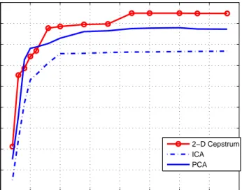
Figure 2.8: Performance Comparison of the Methods for original SAR images of size 128x128
Table 2.5: Confusion Matrix for 2-D cepstrum features BMP-2 T-72 BTR-70 NONE BMP-2 94.02 2.56 2.17 1.26 T-72 4.86 93.86 0.29 0.99 BTR-70 10.42 0.51 89.11 0.04
Table 2.6: Confusion Matrix for PCA features BMP-2 T-72 BTR-70 NONE BMP-2 94.91 1.78 2.03 1.31 T-72 4.52 91.06 2.79 1.63 BTR-70 10.28 0.00 78.16 11.55
Table 2.7: Confusion Matrix for ICA features BMP-2 T-72 BTR-70 NONE BMP-2 91.86 4.18 0.23 3.72 T-72 10.14 87.14 1.29 1.43 BTR-70 25.69 2.08 65.28 6.94
armored personal carriers and T-72 main battle tank are conducted. The target images are of size 128 by 128.
The number of training and test samples used in the classification experi-ments are given in Table 2.4. Training and testing dataset include targets with depression angle 15 and 17 degrees, correspondingly. Due to the SAR imaging system, depression angle has effects on the Signal-to-Noise Ratio (SNR) of the SAR images and may lead to changes in quality of images. Both training and test dataset include target images with evenly distributed orientations angle between 0 and 360 degrees.
In order to use the SVM algorithm on the MSTAR database, the three-class problem was transformed into three two-three-class problems where the positive samples were from one particular class and the rest of the classes formed the negative samples. 2-D cepstral feature parameters are computed from each input image sample as explained in Section 2.4 and they are classified using the SVM with a polynomial kernel. During testing, the classification result is given by the SVM which gave the highest positive output. If all outputs were negative, the sample was rejected, which is indicated by the label ‘None’ in confusion matrices.
The cepstral feature parameters are computed from each input sample as ex-plained in Section 2.4. By converting SAR images into a 1-dimensional vectors
Table 2.8: Average Accuracy Comparison 2-D Cepstrum PCA ICA 128x128 92.30 88.05 81.42 96x96 92.11 90.05 83.27
Table 2.9: Feature Extraction Time Comparison 2-D Cepstrum PCA ICA Time (seconds) 0.025 0.030 0.034
first, we implemented Principal Component Analysis (PCA) and Independent Component Analysis (ICA) in order to obtain the feature vectors correspond-ingly. Feature sets containing 18 and 36 elements are used for PCA and ICA, correspondingly.
Several experiments are performed in order to optimize the grid and weight parameters of 2-D cepstrum method. As it can be seen from Figure 2.8, best recognition rate is obtained using a cepstral feature vector of length 48. Further increase in feature vector size does not improve the performance. Furthermore, it is experimentally observed that regular 2-D cepstrum, which is defined in Equation (3.1), does not give as good results as the proposed 2-D cepstrum method.
Table 2.6 and 2.7 show the confusion matrix results of PCA and ICA methods obtained using SVM. Plots given by Figure 2.8 display the effects of number of features over classification accuracy. For PCA and ICA, increasing the number of significant components after some point (30 for ICA and 45 for PCA) does not improve the performance.
We tried several different kernel functions, however the results were not im-proved with respect to polynomial kernel. The experimental results show that 2-D cepstrum method provide better performance than PCA and ICA. We ex-perimentally observed that even slight changes in target location in SAR images
significantly reduce performance of ICA features. On the other hand, 2-D cep-stral parameters are shift invariant.
Another superior property of 2-D cepstrum feature extraction is that it needs much lower time to compute the features in training stage, as given in the Table 2.3. Furthermore, for 2-D cepstrum approach, time required for extracting fea-tures from a 128 by 128 SAR image in testing stage is lower than than the PCA and ICA methods, as shown in Table 2.9, since 2-D cepstrum feature parameters are computed using the FFT algorithm or the fast DCT algorithm.
Chapter 3
Automatic Target Classification
for Surveillance Pulse-Doppler
Radar
This chapter is organized as follows. In Section 3.1, cepstral analysis meth-ods, which include computation of cepstrum and Mel-Frequency Cepstrum Co-efficients (MFCCs) parameters, are described. In Chapter 2, two-dimensional cepstrum is used. In this chapter, one-dimensional cepstrum is used for feature extraction from radar signals. In Section 3.2, covariance method based approach is explained briefly with its application to radar signals. In Section 3.3, Sup-port Vector Machine (SVM) based approaches are presented. A two-stage SVM based system is developed to classify MFCC parameters in this section. In Sec-tion 3.4, the radar database we use in our experiments is described, experimental classification results obtained by applying the above mentioned methods are pre-sented and compared with Gaussian Mixture Models (GMM) based classification scheme in the radar database.
3.1
Cepstral Analysis
3.1.1
1-D Cepstrum
In [21], the 1-D cepstrum is defined to be the inverse Fourier transform of the log magnitude spectrum of a signal. This is also called as real cepstrum. Tukey defined the cepstrum ˆx[n] of a discrete-time signal x[n] as follows:
ˆ
x[n] = F−1(log(|X(ejw)|)) , (3.1)
where (|X(ejw)|) is the logarithm of the magnitude of the DTFT of the signal
x[n]. In our work, x[n] is the sampled target echo signal.
3.1.2
Mel-Frequency Cepstrum Coefficients (MFCC)
MFCCs are the most important feature parameters in speech recognition and speaker identification. MFCC method is basically a type of cepstrum represen-tation introduced by Davis and Mermelstein [22]. The compurepresen-tation of MFCCs
Figure 3.1: Mel-scale feature extraction
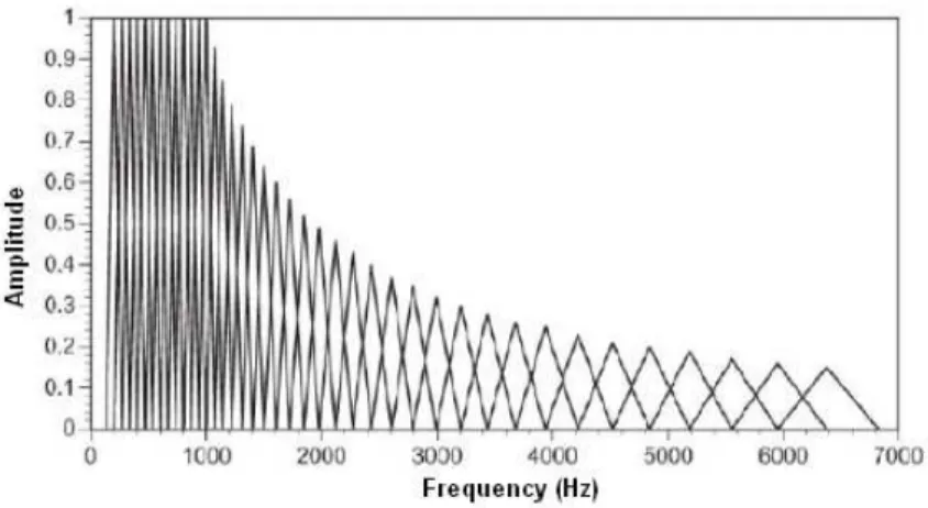
are based on a linear cosine transform of a log power spectrum on a non-linear mel-scale of frequency. Figure 3.1 illustrates a block diagram of extraction of MFCCs from a discrete-time signal. A sample weighting function used in filter
bank, which is named as mel-filter bank, is shown in Figure 3.2. In speech anal-ysis, triangular weighting functions, in other words filters, are mostly used. The use of MFCCs in speech is originated from the analysis of phonetics and human perception of the frequency contents of sounds. For signal processing, MFCCs are commonly derived as follows:
1. Compute the Fourier transform of (a windowed segment of) a signal, 2. Map the powers of the spectrum obtained above onto the mel scale using
shaped (mostly triangular) overlapping windows,
3. Compute the logs of the powers at each of the mel frequencies
4. Compute the discrete cosine transform of the list of mel log powers, as if it were a signal, and
5. Derive the MFCCs as the amplitudes of the resulting spectrum.
Converting frequency f (hertz) into m mel (mapping to mel scale) is done using Equation (3.2) for speech processing. Pre-emphasis stage in Figure 3.1 involves this mapping. There can be variations on this process, for instance, differences in the shape or spacing of the windows used to map the scale [23].
m = 1127 loge(1 + f /700) , (3.2) Consequently, the MFCCs are computed as:
˜ x[i] = N X k=1 Xkcos[i(k − 1 2) π 20], i = 1, 2, ..., M, (3.3) where M is the number of coefficients and Xk, k = 1, 2, ..., N represent the
log-energy output of the kth filter, which are computed using the mel-filter bank illustrated in Figure 3.2.
Figure 3.2: Filters for computing mel-frequency cepstrum co-efficients
3.2
Covariance-based Classification Approach
Porikli et.al introduced the region covariance method as a new image region descriptor, and showed that covariance method is superior to the previous ap-proaches to the object detection and texture recognition problems in some con-text [15]. In case of images, region covariance provides invariance to large ro-tations and illumination changes. We adapted the region covariance approach to radar signal classification. In our scheme, N nonoverlapping and/or overlap-ping segments of t1 miliseconds length radar echo signal construct a classification
frame of T seconds length. If we make an analogy, the pixels in images corre-spond to radar echo segments in our case. Let x be a d-dimensional feature vector for each segment. The vector x may contain the cepstrum or MFCC parameters of a given segment. Let us index the segments using a single index k, and assume that there are N segments in a given classification frame. As a result we have N
d-dimensional feature vectors (xk)k=1...N.
Covariance matrix of the frame is defined as
Σ = 1 N − 1 N X k=1 (xk− µ) (xk− µ)T , (3.4)
The covariance matrices do not lie on Euclidean space. Therefore, since many common machine learning methods operate on Euclidean spaces, they are not appropriate for covariance matrix features. The nearest neighbor algorithm is used as classifier. A generalized eigenvalue based distance metric is used to compare covariance matrices, which was introduced in [24], and used in as a part of the nearest neighbor method:
D(Σ1, Σ2) = v u u tXd k=1 log2λk(Σ1, Σ2), (3.5)
where λk(Σ1, Σ2) are the generalized eigenvalues of covariance matrices Σ1 and
Σ2. The distances between the instance covariance matrix to be classified and the
covariance matrices in the train database are measured. Then, the test instance is assigned to the class of its nearest neighbor.
Covariance matrix combines multiple features which may be correlated. Di-agonal entries of the covariance matrix reflect the variance of each feature and non-diagonal entries reflect the correlations. For radar signals, correlation is an important property to be exploited since consecutive signal segments include information about the same target. Furthermore, averaging operation in the co-variance computation filters out the noise which corrupt the signal. Coco-variance matrix also provides scale invariance [15].
This approach is promising but it is experimentally observed to be inferior to the SVM based approach described in the next section.
3.3
Support Vector Machine Based
Classifica-tion Approach
Recently, SVMs are widely used in classification problems [25]. In this chapter, a two-stage SVM based classification method which employs MFCC features is developed for Pulse-Doppler target classification.
A support vector machine (SVM) [6] estimates decision surfaces directly rather than modeling a probability distribution across the training data. Di-rect application of SVMs yield poor performance on speaker identification and speech recognition, as indicated in [26], in which similarities exist with pulse doppler radar signals. We developed a solution to overcome the direct use of SVMs. Standard Support vector classification gives prediction of only class label
Figure 3.3: Two stage SVM classification scheme
(approximate target value) but not probability information. SVMs can provide probability estimates along with the prediction labels. More details can be found in [20]. These estimates, which give information about the confidence of predic-tion, can be used in classification. Furthermore, SVMs are powerful
discrimina-in classification. Actually, this is the reason why direct application of SVMs performs poor for time-dependent signals. In order to improve the SVM perfor-mance, temporal characteristics should be taken into account. Consequently, we come up with a two-stage solution. We describe this two-stage SVM classification approach in the next sections.
3.3.1
Training of the First Stage SVMs
The aim of this stage is to capture the strongest feature vector representing a given target. For example, the first 5 seconds and the last 20 seconds of the wheeled vehicle have noise-like characteristics and they do not show discrimina-tive behavior as shown in Figure 3.4. Therefore, it is desirable to capture the time segments between 5 and 30 seconds to classify the signal.
In our scheme, radar echo signal is divided into pre-determined number of non-overlapping time intervals of fixed duration. In our case, four time intervals of 5 seconds are used. Then, each interval is divided into segments, which is of 50ms duration in our experiments. From each segment, an MFCC feature vector is computed. A different SVM is trained with MFCC feature vectors computed from the segments of each 5 seconds interval of target signals. So, for each 5 seconds interval, a corresponding SVM is obtained. These SVMs are used to determine the time interval which the test sample best fits.
3.3.2
Training of the Second Stage SVMs
It is assumed that time interval decision is made in the first stage. For each target, 4 different SVMs are trained with the MFCC feature vectors extracted from segments of corresponding time interval. In our case, we have 4 time intervals and therefore, each target has 4 SVMs during training stage. For instance, for
wheeled vehicle target, 4 SVMs are obtained which are for 0-5, 5-10, 10-15 and 15-20 seconds time intervals. Then, if we have 5 targets, 15-20 SVMs are constructed. Since in the first stage, the time interval decision is made, the test sample is inserted into the corresponding second stage SVMs of targets during testing of the second stage. Therefore, only SVMs which corresponds to the decision of the first stage are used in the testing of the second stage.
3.3.3
Testing of the First Stage SVMs
Radar test signal is divided into frames of fixed duration in time. It is reasonable to use frames whose length is smaller than the time intervals used in the training of first stage SVMs. For example, for our case, frames should be smaller than 5 seconds. A decision is made for each frame. Each frame is divided into segments of 50ms duration and from each segment, an MFCC feature vector is computed. For instance, for our case, 100 MFCC feature vectors are obtained from the test frame. These vectors are inserted into the first stage SVMs. Then, the average of the SVM outputs obtained from these vectors, which corresponds to the average of 100 decision values of SVMs, is computed. The test sample is assigned to the class of SVM which gives the highest value. To improve the performance of SVMs, the probability estimates associated with the SVM decision values are used. Therefore, the average of the SVM probability estimates given to each feature vector, is computed and the test sample is assigned to the class of SVM which gives the highest average probability value. Recall that first stage SVMs are used to determine the time interval. Therefore, in this stage, time interval that the test frame belongs to is determined.
3.3.4
Testing of the Second Stage SVMs
In the first stage, time interval decision is established and depending on this decision, corresponding SVMs are used in the second stage. During the training of the second stage SVMs, different SVMs were prepared for each time interval of each target for determining the type of the target. Therefore, depending on the decision of the first stage SVMs, the test feature vector is inserted into the corresponding SVMs of targets. For instance, if it is decided that the test frame is in the 5-10 seconds time interval by first stage SVMs, the MFCC feature vectors of the test frame are inserted to each SVM trained with the MFCC features obtained from the 5-10 seconds time interval of each target. Then, the average of the SVM outputs obtained from these vectors, which corresponds to the average of 100 decision values of SVMs for our case, is computed. The test sample is assigned to the class of SVM which gives the highest value, which is the target type. Again, as in the first stage, average of the probability estimates given by SVMs are used for decision.
3.4
Experimental Results and Discussion
3.4.1
Database Description
The database used in this thesis is collected by a 9 GHz ground surveillance pulse-Doppler radar [27]. The radar has 3 MHz bandwidth, 12 microseconds pulsewidth, 125 meters range resolution and 4 degrees azimuth resolution. Sig-nals in the database are one-dimensional and recorded after down-sampling and filtering of A/D (analog-to-digital) converter of the radar. Sampling rate of the signals are 5.682 KHz.
Figure 3.4: Spectrogram of wheeled vehicle
The recording procedure achieved in a way that the target was detected and tracked automatically by the radar, allowing continuous target echo records. Targets from the following categories were recorded:
• wheeled vehicle, • tracked vehicle, • one person, • two persons and • the vegetation clutter.
Data collection is done in controlled environment and conditions. Experi-ments are conducted under controlled target motions and at high SNR, which means that the range between the radar and the target is relatively short (200 -600 m). For each case, only one target was recorded at a time. In the database, there exist recording of targets having different speeds (for example, depending on the type, slow, normal and fast) and angles of motion toward radar (0,15,30,45,60 degrees).
Figure 3.5: Spectrogram of tracked vehicle
Spectrograms of wheeled vehicle, tracked vehicle, one and two persons and clutter are presented in Figures 3.4 - 3.8. Radar echo signals of sample targets are shown in Figures 3.9 - 3.13. Spectrograms indicate that targets exhibit different time-frequency characteristics which can be exploited for classification.
Target signature may significantly change from one scenario to another for the same target type. Therefore, extensive experiments were carried out in order to obtain the database.
3.4.2
Target Classification Experiments
Classification tests are achieved over a series of signal frames to be classified as one of the possible target classes based on all approaches. In our scheme, N non-overlapping and/or overlapping segments of t1 miliseconds length radar echo
signal constructs a classification frame of T seconds (s) length. A d-dimensional feature vector is extracted from each segment. The feature vector may contain the cepstrum or MFCC parameters of a given segment. In this work, the classification accuracy is used as the criterion for classification performance evaluation. For
Figure 3.6: Spectrogram of clutter
MFCC features, pre-emphasis stage and mel-filter bank (mel filters) are adjusted by analyzing the frequency characteristics of radar target signals.
For GMM-based approach, probability distribution functions (pdfs) of target classes were modeled by GMMs, using Expectation-Maximization (EM) estima-tion algorithms. Both cepstrum and MFCC coefficients are used as classificaestima-tion features. The maximum likelihood (ML) decision concept,which is explained in Section B.0.3, is examined when utilizing GMMs. In case of covariance approach, the covariance of the features are computed using Equation (3.4). As a result, we end up with a covariance matrix, representing each frame. The distances between the instance covariance matrix to be classified and the covariance matrices in the train database are measured and using the distance metric in Equation (3.5), classification is achieved based on the nearest neighbor approach. Therefore, the test instance is assigned to the class of its nearest neighbor. For SVM based approaches, SVMs are trained with the cepstral features and decisions are made over frames. Then, two-stage SVM classification approach, which is explained in Section 3.3, is implemented accordingly and its results are evaluated.
Figure 3.7: Spectrogram of one person
The performances of classification for five-class problem (wheeled vehicle, tracked vehicle, one person, two persons and clutter) are presented. Unless spec-ified, each classification frame of 4 secs length, includes 88 non-overlapping seg-ments of 30 msecs length. We use 4secs length frames since it is a reasonable choice, which can be concluded from the Figure 3.15. A feature vector was ob-tained from each segment. Finally, each frame was classified using 88 feature vectors. The training is achieved with 1496 feature vectors for all target classes. For testing, we use 1056 test frames for all target classes. The classification performance of the GMM-based classifier with both cepstrum and MFCC coef-ficients are illustrated in Figure 3.14. In theory, it is expected that classification accuracy should be improved with increase of the number of features since high order coefficients possess some information on the corresponding target class. However, the parameter estimation performance of the EM algorithm depends on the training database and model order of GMM also affects the performance. Therefore, based on our experiments, it seems that there exists an order of coef-ficients which maximizes the classification accuracy. By investigating the results given in Figure 3.14, it is observed that the maximum classification accuracy is obtained with 6 cepstrum coefficients and 10 MFCC coefficients by GMM-based
Figure 3.8: Spectrogram of two persons
approach. In the next experiments, we use these optimal features for perfor-mance evaluation. Furthermore, the classification accuracy starts to drop after some order of coefficients as seen in Figure 3.14 since the model order is fixed and GMM becomes ineffective in modeling for larger number of features.
Increasing the model order of GMM is not always a solution to the perfor-mance degradation. Thus, the order of coefficients and model order of GMM should be considered and adjusted simultaneously for better performance and there exist limits in the capacity of GMM-based approach. The order of coeffi-cients and model and order of GMM should be established using experiments. Next, the sensitivity of the classification performance of GMM-based approach to the frame length is tested for the above five-class problem. The classification
Wheeled Tracked One Person Two Persons Clutter
Wheeled 74.1 25.9 0 0 0
Tracked 8.2 90.8 0 0 1.0
One Person 0 0 87.3 12.7 0
Two Persons 0 0 2.1 97.9 0
Clutter 0 0 0 5.3 94.7
Table 3.1: Confusion Matrix of GMM Classifier with Cepstrum Coefficients in Five-Class Problem
32.64 32.645 32.65 32.655 32.66 32.665 −1000 −500 0 500 1000 1500 2000 2500 Time (sec) Amplitude Wheeled vehicle 4.95 4.955 4.96 4.965 4.97 4.975 4.98 −2500 −2000 −1500 −1000 −500 0 500 1000 1500 Time (sec) Amplitude Wheeled vehicle 5.61 5.615 5.62 5.625 5.63 5.635 5.64 −2000 −1500 −1000 −500 0 500 1000 1500 Time (sec) Amplitude Wheeled vehicle 31.845 31.85 31.855 31.86 31.865 31.87 31.875 −250 −200 −150 −100 −50 0 50 100 Time (sec) Amplitude Wheeled vehicle
Figure 3.9: Radar echo samples of wheeled vehicle
performance of the GMM classifier with 6 cepstrum and 10 MFCC features is demonstrated in Figure 3.15 as a function of frame length. This figure shows that using frame length between 3 and 5 seconds is a reasonable choice for both cepstrum and MFCC features. On the average, 4 seconds of frame length seems to be an optimal value considering classification accuracy and time allocation to classify a target since it is desired to achieve the classification as quick as possible.
Table 3.1 and 3.2 presents the confusion matrices of GMM-based classifier using cepstrum and MFCC features. We conduct experiments with model order of 10 and feature length 10 for all classes. Using cepstrum and MFCC features, the GMM-based approach achieved classification accuracies of 89.2% and 96.2% correspondingly. Considering the results of these figures and tables, we conclude
0.07 0.075 0.08 0.085 0.09 0.095 −150 −100 −50 0 50 100 Time (sec) Amplitude Tracked vehicle 6.24 6.245 6.25 6.255 6.26 6.265 −1500 −1000 −500 0 500 1000 1500 2000 Time (sec) Amplitude Tracked vehicle 11.585 11.59 11.595 11.6 11.605 11.61 11.615 −400 −300 −200 −100 0 100 200 Time (sec) Amplitude Tracked vehicle 34.65 34.655 34.66 34.665 34.67 34.675 34.68 −500 −400 −300 −200 −100 0 Time (sec) Amplitude Tracked vehicle
Figure 3.10: Radar echo samples of tracked vehicle
that MFCC features outperform cepstrum features in terms of classification ac-curacy. We think that MFCCs provide better representation of the radar target signals by exploiting the frequency bands in spectrum.
Wheeled Tracked One Person Two Persons Clutter
Wheeled 92.1 7.0 0 0 0.9
Tracked 4.1 95.9 0 0 0
One Person 0 0 95.0 5.0 0
Two Persons 0 0 0 100.0 0
Clutter 0 0 0 2.1 97.9
Table 3.2: Confusion Matrix of GMM Classifier with MFCC Coefficients in Five-Class Problem
Next, we achieve experiments in order to compare the results of GMM and co-variance based classification approaches. Table 3.3 presents the confusion matrix of covariance-based approach when 22 MFCCs are used. Covariance approach