Microscopic image classification using sparsity in a transform domain and Bayesian learning

MICROSCOPIC IMAGE CLASSIFICATION USING SPARSITY IN A TRANSFORM

DOMAIN AND BAYESIAN LEARNING

Alexander Suhre

_{, Tulin Ersahin}

_{, Rengul Cetin-Atalay}

_{and A. Enis Cetin}

2_{Department of Molecular Biology and Genetics} Bilkent University,

06800 Bilkent, Ankara, Turkey

Phone: +(90)3122901219, Fax: +(90)3122664192, Email: suhre@ee.bilkent.edu.tr

ABSTRACT

Some biomedical images show a large quantity of different junctions and sharp corners. It is possible to classify several types of biomedical images in a region covariance approach. Cancer cell line images are divided into small blocks and covariance matrices of image blocks are computed. Eigen-values of the covariance matrices are used as classification parameters in a Bayesian framework using the sparsity of the parameters in a transform domain. The efficiency of the proposed method over classification using standard Support Vector Machines (SVM) is demonstrated on biomedical im-age data.

1. INTRODUCTION

Automatic classification of biomedical images is an emerg-ing field, despite the fact that there is a long history of im-age recognition techniques [1]. Automatic classification of carcinoma cells through morphological analysis will greatly improve and speed up cancer research conducted using estab-lished cancer cell lines as in vitro models. Distinct morpholo-gies of different types and even sub-types of cancer cells re-flect, at least in part, the underlying biochemical differences, i.e., gene expression profiles. Moreover, the morphology of cancer cells can infer invasivenes of tumor cell and hence the metastatic capability. In addition, an automated morphologi-cal classification of cancer cells will enable the correct detec-tion and labelling of different cell lines. Cell lines are grown in tissue culture, usually in a lab environment. They repre-sent generations of a primary culture. Although cell lines are being used widely as in vitro models in cancer research and drug development, mislabeling cell lines or failure to recog-nize any contamination may lead to misleading results. Short tandem repeat (STR) analysis is being used as a standard for the authentication of human cell lines. However, automated analysis will provide the scientists a fast and easy-to-use tool that they can use in their own laboratories to verify their cell lines.

In this paper, five classes of biomedical images are classi-fied, namely BT-20, Cama-1, Focus, Huh7 and HepG2 which are all images of cancer cell lines. This is achieved by using an image descriptor based on covariance matrices that are a generalisation of the well-known Harris corner detector to classify images of cells. This approach is used due to the high percentage of junctions in these types of images. The descriptors are computed for small non-overlapping blocks of the images and fed to a Bayesian classification framework that exploits the sparsity of the descriptor’s probability

den-sity functions (PDFs) in a transform domain. In the next section the feature extraction method is described. In Sec-tion 2, the proposed Discrete Cosine Transform (DCT) based Bayesian classification framework is described. Experimen-tal results are presented in Section 4.

2. FEATURE EXTRACTION

Some biomedical images usually show a lot of relatively sharp junctions, as shown in Figures 2. They can be classi-fied according to their edge and corner contents. Therefore, it is wise to select corner detector type features for this kind of biomedical images.

The Harris corner detector [2] is widely acknowledged as a classic feature detection method. It can detect and differen-tiate between corners and edges by examining the principal curvatures in x- and y-direction by evaluating the error be-tween an image region and a shifted version of it, as follows:

c(xi, yj) =

∑

(

I(xi, yj)− I(xi+∆x,yj+∆y) )2

, (1) where W is the window region, I represents the intensity image and (∆x,∆y) denotes the shift in x- and y-direction. Equation 1 can be approximated by

c(xi, yj) = (∆x,∆y) · C(xi, yj)· (∆x,∆y)T, (2) where C(xi, yj) is a 2-by-2 symmetric autocorrelation matrix containing the averaged derivatives in x- and y-directions:

C(xi, yj) =

∑

[Ix(xi, yj), Iy(xi, yj)]· [Ix(xi, yj), Iy(xi, yj)]T (3) where Ix(xi, yj) denotes the derivative of I at (xi, yj) in x-direction. If both eigenvalues of the autocorrelation matrix are high, a corner exists in window W . If only one of the eigenvalues is high and the other is low, an edge is detected. If both eigenvalues are low, the region is found to be flat. The Harris corner detector is largely invariant to rotation, scal-ing, illumination differences and noise. Similar strategies are used in [3], [4]. However, it is experimentally observed that Harris corner detector does not provide good classification results as will be discussed in Section 4.

For this reason the feature vector is augmented to include image intensity and diagonal derivatives as follows:

v(xi, yj) = [I(xi, yj), Ix(xi, yj), Iy(xi, yj), Ix+y(xi, yj), Ix−y(xi, yi)], (4) 19th European Signal Processing Conference (EUSIPCO 2011) Barcelona, Spain, August 29 - September 2, 2011

where the last two entries denote derivatives along the axes at angles of π₄ and 3π₄ with the x-axis, respectively. By in-cluding diagonal derivatives in the feature vector, we can dis-tinguish various types of corners and junctions. In a digital implementation these derivatives can easily be calculated by applying 2-dimensional filters to the image window W . The resulting covariance matrix for a discrete 2-dimensional im-age region W of size M-by-N, can then be written as

C(xi, yj) = 1 MN M

∑

∑

Related work include [5], [6] in which a region descrip-tor based on covariance matrices was used for moving object tracking in video. This framework also uses feature vectors of pixels and constructs a covariance matrix. The feature vector may contain the coordinates of a pixel, its R-, G- and B-Values, derivatives in x- and y-direction or any other prop-erty of a given pixel. The goal of this article is to construct descriptors for cell images, therefore it is sufficient to include only the directional derivatives in the covariance matrix.

3. CLASSIFICATION ALGORITHM

In [7] the differences between discriminative, i.e. paramet-ric, and generative modelling approaches of posterior distri-butions for image classification and object recognition are explored. It is found that generative approaches, while com-putationaly more costy, yield better performance than their discriminative counterparts in general. However, it is usually not straightforward to model a posterior distribution given a set of data. Computing a histogram from the data as an estimate for the posterior distribution may not work due to the limited size of the training data and the resultant unoc-cupied bins in the estimate of the distribution. Unlike [7] no artificial probability models are assumed in order to esti-mate a Bayesian model from the image data. In this paper, a sparse representation in the transform domain of the fea-ture parameter data is assumed. This allows us to fill the missing holes in the distribution in a smooth manner. In the well-known Bayesian estimation problem, the posterior dis-tribution is given by:

p(l|v) = p(v|l)p(l)

∑ip(v|i)p(i)

, (6)

where l denotes the class label and v denotes some feature vector of the image data. In this case, the random vector

v represents the eigenvalues of the region covariance matrix

and all classes are equally likely. If prior distributions are known, one needs to compute the likelihood function in order to find the desired posterior distribution. Therefore, the rest of this section will focus on the likelihood function.

As discussed above, an estimate for the likelihood in Eq. 6 can be obtained easily by computing a histogram from the training data set. However, since a specific v from the test set may not be included in the training set, calculating the likelihood and therefore the posterior distribution for the fea-ture vector in question may not be possible using the his-togram only. The proposed method uses sparse representa-tions of the data histograms in DCT domain to compute an

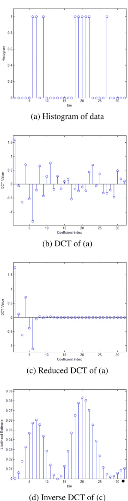
estimate of the full likelihood function. Note that no form of the distribution, e.g. Gaussian, of the data is assumed before-hand. The only assumption is that the conditional PDF have a sparse representation in either Fourier, DCT or wavelet do-main. Using the sparsity of a signal in a transform domain has been widely used in signal processing in digital wave-form coding including JPEG and MPEG family of standards. In recent years, the concept of sparsity is also used to es-timate a given signal from random measurements in com-pressive sensing (CS) [8]. The proposed method uses spar-sity in DCT domain to estimate the conditional PDFs from the histogram of image features. Intuitively, one may ex-pect likelihood functions of continuous random variables ob-tained from natural images as smooth functions, i.e., their representation in Fourier, DCT or wavelet domain is some-what sparse, because natural signals and images are relatively smooth and compressible by DCT based algorithms such as JPEG. In the proposed method, the histogram h(v|l) of each image class is computed from the training set. Then, h(v|l) is transformed into Fourier space or one of its derivatives. In the experiments carried out for this study, the discrete co-sine transform (DCT) which is the most widely used image transformation method is used:

g(Y|l) = DCT{h(v|l)} (7) where g(Y|l) represents the DCT domain coefficient vector (array in multidimensional case). Size of the DCT should be selected larger than the bins of the histogram. The DCT has fast (O(N · logN)) implementations.

Using the sparsity assumption, only the highest q percent of DCT domain coefficients are retained and the remaining DCT coefficients are set to zero. All band-limited signals are of infinite extent in the frequency domain, therefore all the gaps are filled when the reduced ˆg(Y|l) is inverse

trans-formed to its original domain. As in natural images most of the highest q percent of DCT coefficients turn out to be in the low-pass band corresponding to low indexed DCT coef-ficients. This q percent filtered DCT coefficient set is inverse transformed to its original domain and normalized. The re-sultant ˆp(v|l) is an estimate of the unknown likelihood of the

data. The estimated ˆp(v|l) turns out to be smooth functions

because of the low-pass ”filtering” in the DCT domain. Af-ter this estimation step, the posAf-terior probability distribution on the left hand side of Eq. 6 can be readily computed. An example for this method is given in Figure 1. There is the possibility that ˆp(v|l) may contain negative values. One can

then proceed to use an iterative method by setting the nega-tive values to zero and transforming it again to DCT domain, this time retaining the q + #(Iterations) highest DCT coef-ficents, followed by another inverse DCT, until no negative coefficients in the resultant ˆp(v|l) are present. This iterative

method will eventually converge, since it is a projection onto a convex set (POCS) [9].

In the classification step, one image is chosen as test im-age for each class, all other imim-ages of the respective class are assigned as training images, leading to L different classifiers, where L denotes the number of classes. Each test image is fed in a block-by-block manner to one of the L classifiers that were computed from the training set, in order to find a pos-terior probability for each class. For each feature a seperate posterior PDF is computed and results are averaged. Note that by computing seperate PDFs we are not assuming

inde-(a) Histogram of data

(b) DCT of (a)

(c) Reduced DCT of (a)

(d) Inverse DCT of (c)

Fig. 1. Depiction of the algorithm described in Section 3. The histogram in (a) which has empty bins is transformed into (b) using DCT. In (c) the values of the high frequency coefficients are set to zero. The inverse DCT of (c) yields an estimate for the likelihood function that has only non-empty bins, see (d). Note that in (d), bins may have very small likelihood values but larger than zero.

(a) BT-20 class

(b) Cama-1 class

(c) Focus class

(d) HepG2 class class

(e) huh7 class class

pendence of the eigenvalues, as these are computed from a covariance matrix. The block is assigned to the class that yields the largest posterior probability. After all blocks have been fed to the classification process, a final decision for the image is made according to the highest number of class la-bels for the blocks. However, only when at least 50% of all blocks in an image are assigned to one class, is the image classification counted as a success. Although transform do-main methods (e.g. moment generating function) are used in statistics we have not seen any application of transform do-main methods in PDF estimation using sparsity in the trans-form domain to the best of our knowledge.

4. EXPERIMENTAL RESULTS

Two breast and three hepatocellular human carcinoma cell lines are used for the demonstration of the automatic mor-phological profiling of cancer cells. BT-20 is a basal breast cancer cell line (Basal A). It is characterized as an ER-negative invasive ductal carcinoma. Cama-1 is a lumi-nal breast cancer cell line. It is characterized as an ER-positive adenocarcinoma an has been shown to form grape-like colonies with poor cell-to-cell contacts [10]. Luminal A type tumors reflect a good prognostic group, while the Lumi-nal B and basal tumors resemble a bad prognostic group. Fo-cus is a poorly-differentiated mesenchymal-like hepatocellu-lar carcinoma (HCC) cell line. It lacks hepatocyte lineage and epithelial cell markers and instead expresses mesenchy-mal markers. It is high is highly motile and invasive. HCC cell lines have been classified as well- or poor-differentiated according to the indicated markers and migratory features [11], [12]. Huh7 and HepG2 are well-differentiated HCC cell lines with epithelial morphology, displaying low motility and invasiveness. Although they are all adherent cells grow-ing as monolayers, HepG2 cells grow in small aggregates, while Huh7 and Focus tend to cover the entire environment. Some example images of these classes are shown in Figure 2.

The dataset consists of 5 classes with 10 images per class, all taken at 20x magnification. The image size is 4140-by-3096 pixels. Images are divided into small blocks of size 15-by-15 and covariance matrices are computed.

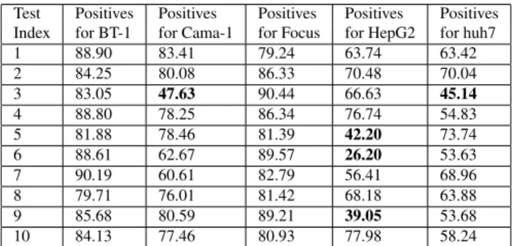
Four experiments are carried out. The first experiment is testing the accuracy of the Bayesian classifier described in Section 3 using the eigenvalues from region covariance ma-trices as features. Results for ten instances can be seen in Ta-ble 1. In this experiment the amount of DCT coefficients that are not set to zero as described in Section 3 is 10%, the his-tograms for each of the eigenvalues is computed over 32768 bins.

The second experiment is very similar to the first exper-iment, only that the features here are the two eigenvalues computed from the Harris corner detector. The classification procedure is exactly as described in experiment 1, however. Results can be seen in Table 2.

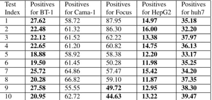
In the third experiment the images are clasified using a standard support vector machine (SVM). For each block, it is determined if the current block is containing background or not. This decision is based on an experimentally standard deviation of the luminance of the given block. If the standard deviation is high, it is regarded as foreground. For the fore-ground blocks the region covariance matrix and its eigenval-ues are computed. The eigenvaleigenval-ues of the foreground blocks

are then put into a multi-class SVM [13], [14] for classifi-cation. The LIBSVM [15] software package is used with a Radial Basis Function (RBF) kernel. Results can be seen in Table 3. It is clear from this table that the SVM approach only yields feasible results for two out of five classes.

The fourth experiment is similar to the third, only that this time around eigenvalues from the Harris corner detector are used in the SVM classifier. Results for the fourth ex-periment can be seen in Table 4, confirming the trend of the other experiemnts that Harris corner features are not feasible for the task at hand.

Test Positives Positives Positives Positives Positives Index for BT-1 for Cama-1 for Focus for HepG2 for huh7

1 88.90 83.41 79.24 63.74 63.42 2 84.25 80.08 86.33 70.48 70.04 3 83.05 47.63 90.44 66.63 45.14 4 88.80 78.25 86.34 76.74 54.83 5 81.88 78.46 81.39 42.20 73.74 6 88.61 62.67 89.57 26.20 53.63 7 90.19 60.61 82.79 56.41 68.96 8 79.71 76.01 81.42 68.18 63.88 9 85.68 80.59 89.21 39.05 53.68 10 84.13 77.46 80.93 77.98 58.24

Table 1. Image block classification accuracies (in %) of eigenvalues from region covariance matrices for the Bayesian classifier. The index of the five test images per class is given in the first column. Block accuracies that led to in-correct classification are printed in bold face. Average image block accuracies are 72.42%, image recognition rate is 90%.

Test Positives Positives Positives Positives Positives Index for BT-1 for Cama-1 for Focus for HepG2 for huh7

1 20.48 3.55 20.19 2.87 42.19 2 5.55 47.33 23.85 18.72 7.06 3 3.81 16.41 14.35 15.98 42.93 4 4.44 78.62 38.00 4.35 14.59 5 14.81 62.46 23.41 5.92 15.87 6 2.01 47.94 8.77 25.61 32.26 7 24.99 15.59 16.71 5.04 49.09 8 8.65 12.91 16.08 20.58 43.61 9 30.65 25.36 2.11 4.99 36.43 10 14.06 15.21 13.33 2.52 39.18

Table 2. Image block classification accuracies (in %) of eigenvalues from Harris corner detector for the Bayesian classifier. The index of the five test images per class is given in the first column. Block accuracies that led to incorrect classification are printed in bold face. Average image block accuracies are 21.23%, image recognition rate is 4%.

5. CONCLUSION

It is demonstrated that the region covariance matrix can be used for automatic classification of certain cancer cell line images in a Bayesian classification framework. The two main findings of this paper are the following:

1. For the application at hand, the classification method developed in this paper yields better results than the

Test Positives Positives Positives Positives Positives Index for BT-1 for Cama-1 for Focus for HepG2 for huh7

1 27.62 58.72 87.95 14.97 35.18 2 22.48 61.32 86.30 16.00 32.20 3 22.12 61.52 62.22 13.38 37.97 4 22.65 61.20 60.82 14.75 36.13 5 18.88 58.92 58.38 12.20 33.17 6 19.50 61.45 50.28 11.98 35.25 7 25.72 64.86 57.47 15.42 34.20 8 20.28 66.82 59.10 11.87 37.35 9 27.58 55.55 49.72 12.95 38.30 10 20.95 62.72 44.63 13.22 39.47

Table 3. Image block classification accuracies (in %) of eigenvalues from region covariance for the SVM classifier. The index of the five test images per class is given in the first column. Block accuracies that led to incorrect classification are printed in bold face. Average image block accuracies are 39.07%, image recognition rate is 36%.

Test Positives Positives Positives Positives Positives Index for BT-1 for Cama-1 for Focus for HepG2 for huh7

1 00.00 47.47 90.55 00.00 44.40 2 00.00 42.33 88.87 00.00 47.53 3 00.00 48.18 72.90 00.00 49.03 4 00.00 47.57 71.10 00.00 46.42 5 00.00 48.33 67.97 00.00 50.27 6 00.00 46.33 60.63 00.00 42.88 7 00.00 50.18 61.03 00.00 42.17 8 00.00 51.27 64.85 00.00 44.48 9 00.00 39.90 54.47 00.00 48.75 10 00.00 45.25 51.58 00.00 48.62

Table 4. Image block classification accuracies (in %) of eigenvalues from Harris corner detector for the SVM clas-sifier. The index of the five test images per class is given in the first column. Block accuracies that led to incorrect classification are printed in bold face. Average image block accuracies are 32.33%, image recognition rate is 26%.

straightforward application of the popular SVM classi-fier.

2. Eigenvalues from region covariance matrices are better suited descriptors for the image classes under investiga-tion than the Harris corner detector.

Future work may include comparisons of the eigenvalues of region covariance matrices with SIFT features. The proposed Bayesian approach is original because parts of the PDFs of the image feature data are estimated in transform domain us-ing the well-known DCT.

6. ACKNOWLEDGMENTS

This study was funded by the Seventh Framework program of the European Union under grant agreement number PIRSES-GA-2009-247091: MIRACLE - Microscopic Image Process-ing, Analysis, Classification and Modelling Environment.

REFERENCES

[1] M. M. Dundar, S. Badve, V. C. Raykar, R. K. Jain, O. Sertel, and M. N. Gurcan, “A multiple

in-stance learning approach toward optimal classification of pathology slides,” Pattern Recognition, Interna-tional Conference on, vol. 0, pp. 2732–2735, 2010.

[2] C. Harris and M. Stephens, “A combined corner and edge detector,” in Proceedings of the 4th Alvey Vision

Conference, 1988, pp. 147–151.

[3] D. G. Lowe, “Distinctive image features from scale-invariant keypoints,” International Journal of Com-puter Vision, vol. 60, pp. 91–110, 2004.

[4] Y. Bastanlar and Y. Yardimci, “Corner validation based on extracted corner properties,” Computer Vision and

Image Understanding, vol. 112, pp. 243–261, 2008.

[5] O. Tuzel, F. Porikli, and P. Meer, “Region covariance: A fast descriptor for detection and classification,” in In

Proc. 9th European Conf. on Computer Vision, 2006,

pp. 589–600.

[6] H. Tuna, I. Onaran, and A. E. Cetin, “Image description using a multiplier-less operator,” IEEE Signal

Process-ing Letters, vol. 16, pp. 751–753, 2010.

[7] Christopher M. Bishop and Ilkay Ulusoy, “Object recognition via local patch labelling,” in in Workshop

on Machine Learning, 2005.

[8] Richard G. Baraniuk, “Compressive sensing,” Lecture

Notes in IEEE Signal Processing Magazine, vol. 24, no.

4, pp. 118–120, Jul. 2007.

[9] P.L. Combettes, “The foundations of set theoretic esti-mation,” Proceedings of the IEEE, vol. 81, no. 2, pp. 182 –208, 1993.

[10] P. A. Kenny, G. Y. Lee, C. A. Myers, R. M. Neve, J. R. Semeiks, P. T. Spellman, K. Lorenz, E. H. Lee, M. H. Barcellos-Hoff, O. W. Petersen, J. W. Gray, and M. J. Bissell, “The morphologies of breast cancer cell lines in three-dimensional assays correlate with their profiles of gene expression,” Mol Oncol., vol. 1, no. 1, pp. 84– 96, 2007.

[11] B. C. Fuchs, T. Fujii, J. D. Dorfman, J. M. Goodwin, A. X. Zhu, M. Lanuti, and K. K. Tanabe, “Epithelial-to-mesenchymal transition and integrin-linked kinase me-diate sensitivity to epidermal growth factor receptor in-hibition in human hepatoma cells,” Cancer Res., vol. 68, no. 7, pp. 2391–9, 2008.

[12] H. Yuzugullu, K. Benhaj, N. Ozturk, S. Senturk, E. Ce-lik, A. Toylu, N. Tasdemir, M. Yilmaz, E. Erdal, K. C. Akcali, N. Atabey, and M. Ozturk, “Canonical wnt sig-naling is antagonized by noncanonical wnt5a in hepa-tocellular carcinoma cells,” Mol Cancer, vol. 8, no. 90, 2009.

[13] C. J. C. Burges, “A tutorial on support vector machines for pattern recognition,” Data Mining and Knowledge

Discovery, vol. 2, pp. 121–167, 1998.

[14] A. Eryildirim and A. E. Cetin, “Pulse doppler radar target recognition using a two-stage svm procedure,”

IEEE Transactions on Aerospace and Electronic Sys-tems, 2010.

[15] Chih-Chung Chang and Chih-Jen Lin, LIBSVM: a

li-brary for support vector machines, 2001, Software available at http://www.csie.ntu.edu.tw/ cjlin/libsvm.