An actuated flexible spinal mechanism for a bounding quadrupedal robot

(1)

a thesis

submitted to the department of computer engineering

and the graduate school of engineering and science

of bilkent university

in partial fulfillment of the requirements

for the degree of

master of science

By

Utku C

¸ ulha

January, 2012

(2)

I certify that I have read this thesis and that in my opinion it is fully adequate, in scope and in quality, as a thesis for the degree of Master of Science.

Assist. Prof. Dr. Ulu¸c Saranlı(Advisor)

Assist. Prof. Dr. Melih C¸ akmak¸cı

Assist. Prof. Dr. Selim Aksoy

Approved for the Graduate School of Engineering and Science:

Prof. Dr. Levent Onural Director of the Graduate School

(3)

FOR A BOUNDING QUADRUPEDAL ROBOT

Utku C¸ ulha

M.S. in Computer Engineering Supervisor: Assist. Prof. Dr. Ulu¸c Saranlı

January, 2012

Evolution and experience based learning have given animals body structures and motion capabilities to survive in the nature by achieving many complicated tasks. Among these animals, legged vertebrates use their musculoskeletal bodies up to the limits to achieve actions involving high speeds and agile maneuvers. More-over the flexible spine plays a very important role in providing auxiliary power and dexterity for such dynamic behaviors. Robotics research tries to imitate such dynamic abilities on mechanical platforms. However, most existing robots per-forming these dynamic motions does not include such a flexible spine architecture. In this thesis we investigate how quadrupedal bounding can be achieved with the help of an actuated flexible spine. Depending upon biological correspondences we first present a novel quadruped robot model with an actuated spine and relate it with our proposed new bounding gait controller model. By optimizing our model and a standard stiff backed model via repetitive parametric methods, we investigate the role of spinal actuation on the performance enhancements of the flexible model. By achieving higher ground speeds and hopping heights we discuss the relations between flexible body structure and stride properties of a dynamic bounding gait. Furthermore, we present an analytical model of the proposed robot structure along with the spinal architecture and analyze the dynamics and active forces on the overall system. By gathering simulation results we question how such a flexible spine system can be improved to achieve higher performances during dynamic gaits.

Keywords: Bio-inspired robotics, Legged robots, Dynamic Locomotion, Quadrupedal bounding, Spinal actuation, Gait optimization.

(4)

¨

OZET

SIC

_{¸ RAYARAK KOS.AN D ¨}

ORT BACAKLI B˙IR ROBOT

˙IC¸˙IN KONTROL ED˙ILEB˙IL˙IR ESNEK BEL OMURGA

MEKAN˙IZMASI

Utku C¸ ulha

Bilgisayar Mühendisli˘gi, Yüksek Lisans Tez Yöneticisi: Assist. Prof. Dr. Ulu¸c Saranlı

Ocak, 2012

Evrim ve tecrübe tabanlı ö˘grenme süreci hayvanlara do˘gada hayatta kalabilmeleri i¸cin bir¸cok karmas.ık görevi yerine getirebilen vücut yapıları ve hareket kabiliyet-leri vermis.tir. Bu hayvanlar arasında özellikle bacaklı omurgalılar, yüksek hızlara eris.mek ve keskin manevralar yapabilmek i¸cin kaslı iskelet vücut yapılarını kul-lanırlar. Buna benzer dinamik davranıs.larda esnek omurga, havyana fazladan gü¸c ve esneklik deste˘gi vererek ¨_{onemli bir rol oynamaktadır. Robotik aras.tırmaları} buna benzer dinamik becerileri mekanik sistemlerde g¨_{osterebilmeyi amac.lar.} Buna ra˘gmen günümüzde benzeri dinamik hareketleri yapabilen robotlar esnek omurga sistemlerine sahip de˘gillerdir. Biz bu tez ile kontrol edilebilir omurga sisteminin d¨_{ort bacaklı robotlarda sı¸crayarak kos.ma hareketi üzerindeki etkilerini} aras.tırıyoruz. Biyolojik kaynaklara dayanarak, ilk olarak yeni bir kontrol edilebilir omurgaya sahip dört bacaklı robot modeli sunuyor ve bu modeli yine yeni olarak sundu˘_{gumuz sı¸crayarak kos.ma kontrolü modeli ile ba˘gdas.tırıyoruz. C}¸ ok tekrarlı de˘_{gis.kenli yöntemler kullanarak, sundu˘gumuz esnek robot ve standart robot} mod-elini eniyiles.tiriyor ve bununla beraber omurga kontrolünün sundu˘gumuz es-nek robot modeli ¨_{uzerindeki bas.arım etkilerini aras.tırıyoruz. Daha yüksek hız} ve zıplama yükseklikleri elde ederek esnek vücut yapısı ile dinamik sı¸crayarak kos.ma hareketinin adım özellikleri arasındaki ba˘gı inceliyoruz. Ayrıca tezimizde, sundu˘gumuz robot modelinin ve robottaki omurga sisteminin analitik incelemesini yaparak, büt¨_{un sistemdeki dinamikleri ve kuvvetleri aras.tırıyoruz. Simülasyon} sonu¸clarına bakarak esnek bir omurga sisteminin, robotlardan daha yüksek verim alabilmek i¸cin ne dereceye kadar gelis.tirilebilece˘gini sorguluyoruz.

Anahtar s¨ozc¨_{ukler : Biyolojiden esinlenmis. robotlar, Bacaklı robotlar, Dinamik}

hareket, D¨_{ort bacakla sı¸crayarak kos.ma, Omurga kontrolü, Yürüyüs. eniyiles.tirme.} iv

(5)

I would like to thank my supervisor Ulu¸c Saranlı for guiding me through my bachelor and graduate years in my university and giving me his vision, insight and understanding of academics with his utmost energy for this 7 year period. I can honestly say his provision has shaped my career in robotics and possibly the rest of it and I am gladly thankful for all of his eﬀorts so far and so will I be in the rest of my career for he played a very important initiative role.

I wish to acknowledge Melih C¸ akmak¸cı and Hartmut Geyer in providing cre-ative ideas and support during the initiation of this project and showing me pos-sible directions about how my research can be extended for many future paths.

I would also like to thank Fırat ˙Ilhan for his guidance and help on academic decisions in my career. His intellectual and technical knowledge and friendship have been very important in both my social and professional life, for which I am gladly thankful.

I want to thank all my colleagues in Bilkent Dexterous Robotics and Loco-motion (BDRL) group because of their never ending motivation and energy for keeping the research alive and fruitful.

Most importantly, I am grateful to my family who supported me anytime and believed in me since the beginning. It would be impossible without their support to complete any of my duties and fulﬁlling my ideas including this research. Therefore it will be my pleasure to dedicate this research to my lovely family.

(6)

List of Figures

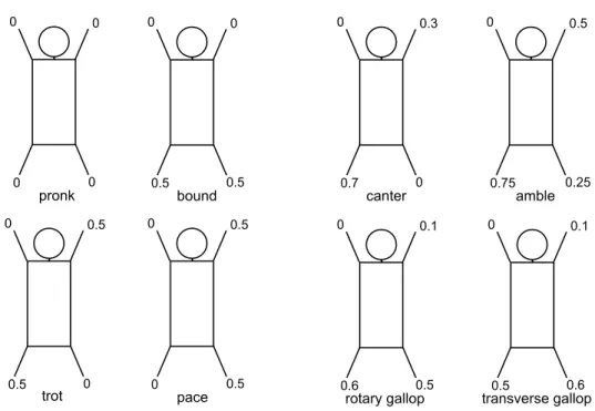
2.1 Quadrupedal gait types inspired from Alexander’s work. The group on the left shows symmetrical patterns, while the four gait types on the right have asymmetric periods for each leg. . . 7 2.2 Two diﬀerent planarized bounding models. (left) The ﬁrst model

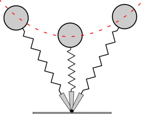
assumes that there could be at most one leg on the ground at a time. (right) The second model has a double stance phase. . . 9 2.3 The Spring-Loaded Inverted Pendulum (SLIP) model, showing an

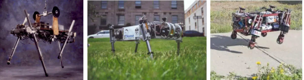
example trajectory of the point mass during stance. . . 10 2.4 Raibert’s quadruped (left), SCOUT II platform (middle), PAW

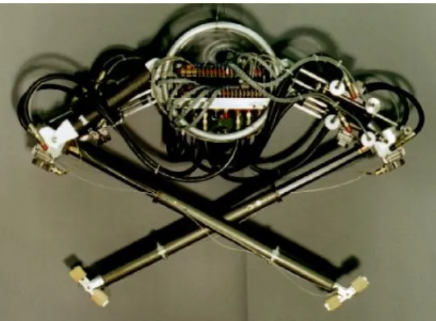
robot (right) . . . 11 2.5 Leeser’s planar quadruped with an articulated spine. All actuation

is done through hydraulically-powered motors. ( Figure adapted from [18] ) . . . 13

3.1 The planar quadruped robot model with passively compliant legs and a stiﬀ body structure. . . 19 3.2 The proposed planar quadruped model with an actuated spine joint

and hip actuated compliant legs attached. The model is inspired from nature in order to increase the dynamic gait performance of the robot. . . 20

(11)

3.3 Two phases of the ﬂexible spine; concave (left) and convex (right) 21 3.4 Flexible back (left) and stiﬀ back (right) planar robot models

cre-ated in Working Model 2D environment. The stiff-backed model has an anchor constraint between two body segments. . . 23 3.5 The new bounding gait model with different poses of the flexible

spine in our new model. . . 24 3.6 Trajectory generation system shown for an angle control in a stance

phase of a leg. Compared to step change (left), trajectory tracking (right) updates φ∗_i(t) in each time step with respect to slope or ˙φi. 30

3.7 Progression of the Nelder-Mead optimization for stiff backed (left) and actuated spine (right) models. Red squares plot the stop-ping criteria function C, whereas blue stars represent the best ver-tex cost values for each simplex. Each “turn” corresponds to five Nelder-Mead iterations. . . 34 3.8 Snapshots of stiff backed bounding model during Working Model

2D simulations. . . 37 3.9 Leg lengths (top) and body pitch angle (down) for the stiﬀ backed

bounding model. . . 38 3.10 Body height (top), horizontal velocity (middle) and foot clearance

(bottom) trajectories for bounding with the stiﬀ-backed model. Green dashed lines in the top two plots indicate the average hor-izontal speed and heights. Shaded regions in the bottom indicate diﬀerent controller phases. . . 39 3.11 Leg angles of the back leg (dashed blue line) and the front leg (solid

(12)

LIST OF FIGURES xii

3.12 Power consumption (top) and torque output (bottom) of motors. Blue dotted line represents front hip motor and black line back hip motor. . . 40 3.13 Snapshots of the ﬂexible backed bounding model during Working

Model 2D simulations. . . 41 3.14 Leg lengths (top) and body part pitch angles (bottom) of ﬂexible

bounding gait model. . . 42 3.15 Body height (top), horizontal velocity (middle) and foot clearance

(bottom) trajectories for bounding with the actuated spine model. Green dashed lines in the top two plots indicate the average hor-izontal speed and heights. Shaded regions in the bottom indicate diﬀerent controller phases. . . 43 3.16 Angular trajectory of the legs (top) and the spine (bottom) during

bounding motion. . . 44 3.17 Power consumption (top) and torque output (bottom) of hip and

spine actuators. Red dashed line represents the spine motor, blue dotted line front hip motor and black line back hip motor. . . 45 3.18 Stride lengths for the back (left plot) and front (right plot) legs for

the last six bounding steps. Red stars illustrate stride lengths for the actuated spine model whereas the blue squares correspond to the stiﬀ backed model. . . 46 3.19 Leg springs’ reaction forces on the ground comparing the stiﬀ

backed and ﬂexible backed model. The front legs (top) and back legs (bottom) are compared. . . 48

4.1 Planar quadrupedal robot model with an actuated spine joint con-necting two body segments. Parameters shown on the robot deﬁne kinematic relations and properties. . . 53

(13)

4.2 Kinematic relationships on a single leg. . . 55 4.3 Free body diagram of the robot showing relevant forces and torques. 57 4.4 Viscous friction force as a function of total horizontal force on the

toe, Fx. . . 67

4.5 An alternative ﬂexible bounding gait in which four consecutive phases follow each other, guaranteeing that only one leg can be in stance at a time. Therefore there are no double stance phases. . . 69 4.6 Center of mass height (top), center of mass horizontal velocity

(middle) and feet clearance with gait cycle phases (bottom) of the ﬂexible backed robot model. Green dashed lines in top two graphs show the average values. . . 76 4.7 Angular trajectory of the spine during bounding motion. . . 77 4.8 Instantaneous power consumption (top) and torque output

(bot-tom) of hip motors during bounding gait. . . 77 4.9 Instantaneous power consumption (top) and torque output

(bot-tom) of spine motor during bounding gait. . . 78 4.10 Rotational velocity (top) and position (bottom) of each hip joint

during bounding gait. . . 81 4.11 Torque output of the spine motor in a single stride that consists

(14)

List of Tables

3.1 High-level state machine for stiﬀ-backed bounding. . . 27

3.2 High-level state machine for ﬂexible backed bounding. . . 28

3.3 System parameters for both bounding models. . . 31

3.4 Optimal gait parameters for Stiﬀ Backed Bounding . . . 35

3.5 Optimal gait parameters for Actuated Spine Bounding . . . 36

3.6 Speciﬁc resistance values for bounding behaviors. . . 50

4.1 Kinematic parameters for body segments. . . 54

4.2 Kinematic parameters for leg parts. . . 54

4.3 Parameter names and deﬁnitions for forces acting on joints. . . 58

4.4 Optimal gait parameters for actuated spine bounding of the math-ematical model . . . 74

(15)

Introduction

1.1 Dexterous Robotics and Locomotion

As a result advances in materials science and manufacturing and production of actuation technologies, it has become easier to design and build robots that are more mobile and eﬃcient and that can be used in many diﬀerent areas in daily life. Currently, mobile and dexterous robots have been used in various tasks such as search and rescue, rehabilitation, surgical operations, exploration and many others where human intervention could be risky or unnecessary [29]. The need for robots increases in parallel with improvements in robotics technology. While robots become more complex and their sets of skills increase, the desired actions that they are asked to complete are also becoming more complex.

However, in almost all of these domains, locomotion, or the action of moving the subject body from one point to another, is one of the most important parts of the whole task. The method used for locomotion also depends on the desired duty of the robot. While many robotic platforms prefer to use wheels due to a large body of knowledge and experience on the design of their structure and control, a relatively new research area focuses on the usage of legs in robots, in manners similar to how they are used in nature.

(16)

CHAPTER 1. INTRODUCTION 2

From this perspective, inspiration from nature plays a very important role in designing leg structures for robots in order to succeed in performing locomotion tasks that might occur frequently in robotic applications. When high speed and maneuverability are required, there are many striking examples in nature which successfully demonstrate the agility of leg morphologies [15]. Animals from the cat family such as leopards and cheetahs and other mammals such as gazelles and goats demonstrate very high performance while running with high speeds, or avoiding obstacles during locomotion. These animals also use their leg and muscle morphologies in the most efficient way to minimize energy consumption, resulting in efficiency in catching their preys or running away from their predators on complex and unstructured outdoor environments [33]. When locomotion patterns and behaviors of these animals are investigated, it is found that the agility of such maneuvers depends on how they maintain balance during their motion. Compared to static balance requirements, where the center of mass of the subject body must stay inside a triangle formed by the group of legs touching the ground at the same time, dynamic balance does not impose such constraints. For different locomotion gaits performed by these animals, there are phases of the gait when none of the legs are touching the ground, but the animal is still in balance. As a result, these animals can run with high speeds and overcome obstacles by jumping high in the air. For these reasons, many researchers in the robotics field have been inspired from these animals and their legged morphologies to create their own bio-inspired multi-legged robots capable of performing gaits based on dynamic balance [29].

Quadrupedal animals in nature adapt different dynamic gaits due to the re-quirements of different tasks and actions. Considering locomotion in general, gaits are classified with respect to the periods of each leg’s event of touching the ground. As these events happen periodically, the whole gait can be represented by only one period, showing the event times in one stride. While some quadrupedal gaits like amble, canter and gallop have asymmetrical patterns with respect to leg events, some gaits like trot, pace, bound and pronk have symmetrical leg patterns [1]. Due to differing advantages and disadvantages of each of these gaits, animals

(17)

prefer to switch between them during their locomotion. For example, while gal-loping lets the animal achieve high speeds, bounding and pronking decrease the speed but enable jumping over high obstacles.

Among these dynamic locomotion gaits, bounding stands out with its sym-metrical pattern and its maneuverability. In nature, most quadrupedal animals switch to the bounding gait in order to achieve obstacle avoidance in moderate speeds [6]. The symmetrical pattern of the gait has also caught the attention of most robotics researchers because it allows easy implementation with complex mechanisms and control systems. Furthermore, by reducing this gait into simple phases, many quadruped robots have performed bounding by using simple control strategies and leg structures [13, 17, 24, 31].

When all current quadruped robots capable of dynamic locomotion gaits are investigated, it can be seen that nearly all approaches focus on the structure and design of the legs, the complexity and robustness of the control systems or the type of actuation used in the mechanism. Even though these robots are inspired from natural examples, one of the major mechanisms in animals seems to be missing in the implementations: the flexible spine. Some of the fastest and most agile land running mammals use their flexible spine to enhance their performance and energy efficiency during high speed locomotion. The musculoskeletal spine acts as a compliant mechanism to increase the body flexibility, as well as an intermittent unit to transfer energy from front muscles to back or vice versa [3]. It is also used like a spring to give additional thrust to the subject body for jumping tasks [20].

By observing the eﬃciency of spinal ﬂexibility in nature and locomotion per-formance of mentioned robotic applications, the question of how such a compliant mechanism can be implemented for quadrupedal robots. The literature in this do-main contains few attempts to answer this question by implementing an actuated or passive spine structure to enhance dynamic locomotion gaits used [18, 32]. Even though the idea of implementing a spine mechanism similar to animals sounds trivial, the researchers have focused on solving more basic problems in

(18)

CHAPTER 1. INTRODUCTION 4

locomotion such as leg designs and controller systems. However, the state-of-the-art robotic systems can now provide a large range of solutions to these problems and the literature in this ﬁeld has a big volume. Therefore, by depending on the brought solutions to previous problems, it is now easier to focus on the question of spinal actuation and its eﬀects on dynamic locomotion.

1.2 Contributions

Our main contributions in this thesis are to first introduce a proof of concept model for a spinal actuation mechanism for a planar quadruped robot, running with a bounding gait. This model addresses the question of how a flexible spine could enhance the locomotion performance compared to a stiff trunk. Along with this concept, a new bounding controller that fits this flexible spine model has also been proposed. The comparison of a state-of-the-art stiff backed quadruped model and a newly proposed flexible spine model, running according to a widely used bounding model and the proposed new bounding model has been presented [9]. It is shown that the proposed structure and controller for a flexible spine increases locomotion performance for horizontal body speed and jumping heights both of which are found to be the results of increased stride length.

This thesis expands this concept’s contribution by also introducing a detailed mathematical model of a planar quadruped robot model with a ﬂexible spine. We derive the equations of motion for this new spinal mechanism and ﬁnd various forces acting on the spine and legs. This derivation also enables us to investigate spinal thrust and necessary compliant mechanisms to enhance the locomotion performance as well as decreasing the power costs.

As an overview this thesis proves the positive effects of using a flexible spine mechanism as in a manner similar to how it is used in many mammals, by com-paring simulation results of a stiff backed quadruped robot with those of the proposed flexible backed robot.

(19)

1.3 Thesis Organization

In Chapter 2 we brieﬂy give background information related to the scope of this thesis. The chapter explains dynamic locomotion gaits used in animals and bio-inspired robots. Then, we focus on bounding gait and present its widely used and accepted control models. This chapter also gives examples from robotic applications on bounding gait and the usage of ﬂexible spine in quadrupedal locomotion. We also explain major gait optimization techniques and focus on the Nelder and Mead optimization algorithm which we used to optimize the parameter set of our quadrupedal models.

In Chapter 3, we describe our proof of concept for a quadruped robot with an actuated spine. In this chapter, the structural model of the robot, the newly proposed bounding gait controller model, and the comparative simulation exper-iments done are presented and evaluated.

Chapter 4 presents analytical derivation of equations of motion of ﬂexible quadruped model which gives information about dynamics and forces acting on legs and spine. Additional features such as leg retraction and ground friction are also explained. Simulations done with this model and their results are explained at the end of this chapter, along with the discussion of the overall mechanism.

In the last Chapter 5 we give a summary of what we have presented in the thesis and suggest further expansions our research.

(20)

Chapter 2 Background

2.1 Locomotion Gaits

2.1.1 Major Gait Types

Animals have adapted different locomotion types through evolution and learning through experience. Even though animals differ greatly in size, functionality and form, a big portion of them use common locomotion gaits. These gait types can be classified with respect to the duration of feet contact with the ground and the symmetry of events within a single stride [1].

Alexander describes a single stride in the whole gait as a complete cycle of leg events starting from the touching down of one particular leg until its next touchdown and all other legs touching the ground only for once during this period [1]. He also uses a descriptor called dutyf actor of a foot β, which denotes the fraction of a whole stride period for which the foot is on the ground. Considering this factor, he selects a reference foot, which is generally the fore left foot, and describes diﬀerent types of gaits in quadrupedal mammals as in Figure 2.1.

It can be seen from the ﬁgure that amble, canter and gallops show asymmetric patterns as each foot spends a diﬀerent duration on the ground. However, other

(21)

Figure 2.1: Quadrupedal gait types inspired from Alexander’s work. The group on the left shows symmetrical patterns, while the four gait types on the right have asymmetric periods for each leg.

gait types represent symmetrical patterns. Diﬀerences in each gait also brings diﬀerent advantages. While animals prefer symmetric gaits for slow speeds but complex maneuvers, asymmetric gaits are generally preferred to achieve higher speeds on dynamically stable tracks. Picturing a horse running at high speeds with a rotary gallop and an antelope jumping over high obstacles using the pronk-ing gait can give the reader an idea about the usage of these gaits.

In robotics, symmetric gaits are generally more preferred than asymmetric gaits. The reason for such a choice lies within the simplicity of representing a single stride with less complexity. This low complexity also helps researchers to identify gait controllers on reduced space dimensions since groups of legs having identical event durations and triggers can be represented as a single leg. For example, as all of the legs in the pronking gait act identically within the stride, all 4 legs can be represented as a single leg [2]. Also, legs on the same diagonal line in the trot gait or legs on the same side of the body in the pace gait can reduce control complexity in the overall system [27].

(22)

CHAPTER 2. BACKGROUND 8

2.1.2 A Gait Model For Bounding

Compared to the other dynamic locomotion gaits, bounding is the most imple-mented on robotic platforms. Due to its symmetrical pattern and coupled event maps for front and back legs, bounding reduces control complexity. However, in order to understand the advantages of this gait, one must analyze the mechanics of phases within a single stride of bounding.

First of all, the most appealing features of this gait is the coupled use of the front and back legs [1]. In quadrupedal bounding, we see that both of the front legs have exactly the same periods of motion within the overall stride. In other words, they touch the ground at the same time, and leave the ground at the same time. This is also true for the two back legs. When this symmetry is considered, quadrupedal bounding becomes very easy to be restrict to the sagittal plane for analysis.

The planarization of quadrupedal bounding reduces the dimension of the prob-lem from a 3D world into a planar, 2D world [26]. In a planar world, a pair of legs can be represented by only a single leg, which is a very eﬃcient way of modeling bounding. As bounding has the leg symmetry, the front legs and the back legs of the quadruped can be summarized with a single leg for each corresponding pair. This also reduces the number of controllers for each leg, as only one controller will be needed to control each leg pair, which are now combined into a single leg on the sagittal plane.

Considering this planarization, bounding has been represented by two diﬀer-ent approaches so far. Both of the approaches are widely used by many robotics platforms due to their low level of complexity. Both of these methods represent a single stride of bounding in four consecutive phases. Moreover, each method relies on the detection of each leg contact event and change their controller pa-rameters and strategies accordingly. Major events that need to be detected are the touchdown and liftoﬀ of each leg pair. By only depending on these leg events, none of these bounding gait controllers need to consider the state of the body explicitly. Detecting these two events for each leg, both models achieve successful

(23)

dynamic locomotion via bounding.

The first method [2] assumes that there can be only one leg touching the ground at a time. Consequently, every time a leg touches the ground and leaves it afterwards in the half of the stride period, the other leg is controlled for touchdown for the rest of the stride. On the left part of Figure 2.2, this controller’s state machine can be seen. Although this gait controller has 4 visible phases, it has two switching controller states. Whenever the current controlled leg leaves the ground after the liftoff event, the controller switches to the other leg to complete another cycle. By using this strategy, the same controller with different parameters can be used for each leg by only detecting the touchdown and liftoff events.

The alternate method, [23], includes a double stance phase, hence differing from the first method. As it can be seen from Figure 2.2, the state machine shown on the right shows a double stance phase which is triggered by the touchdown event of back leg, which happens before the liftoff event of the fore leg.

Figure 2.2: Two diﬀerent planarized bounding models. (left) The ﬁrst model assumes that there could be at most one leg on the ground at a time. (right) The second model has a double stance phase.

2.1.3 Legged Robots Capable of Dynamic Bounding

Some of the ﬁrst contributions to bio-inspired legged robot research were done by Raibert et al. [26], based on a dynamic model of a single leg. The Spring-Loaded Inverted Pendulum (SLIP) model, was found to be very close in performance

(24)

compared to animal legs when active forces and dynamics are investigated. As implied by the name, the SLIP model consists of a point mass attached to a spring, which touches the ground on the other end. Very similar to the dynamics of an inverted pendulum, the overall body acts as an elastic pendulum on the ground. When the tip of the spring touches the ground, the kinetic energy on the point mass starts to be converted into potential energy, which is stored in the compliant leg mechanism during stance. While the spring gets compressed due to active forces, the point mass follows a sinusoid-like trajectory. When the spring is in the full compression, the body mass reaches its lowest height on the overall trajectory. After that point, the potential energy stored on the spring mechanism starts to be transferred into kinetic energy with the leg entering its thrust phase. Figure 2.3 shows an example trajectory of this model throughout a single stride.

Figure 2.3: The Spring-Loaded Inverted Pendulum (SLIP) model, showing an example trajectory of the point mass during stance.

Despite being an approximation, the SLIP model has been and is still being used as the basis for most hip actuated robot designs. One of the most important aspects of this model is its simplicity. The leg itself is composed of a compliant spring, so the contraction and retraction phases of the leg on the ground can be maintained by the nature of spring dynamics without any external controls. Leaving the ground dynamics of the leg to the passive spring, the only control needed for the whole leg is for the hip joint which connects the leg rod onto the body. This hip actuator’s job is to control the position of the leg with respect to the body and adjust an angle diﬀering with respect to the phases of a dynamic

(25)

gait. Raibert’s quadruped robots use this basic design to achieve diﬀerent dy-namic gaits such as trotting, pacing and bounding [27]. He incorporates two levels of control for quadrupedal bounding. The high-level controller for gait phases de-cides on desired angles for legs for touchdown and liftoﬀ events. This controller is independent of body state, but only acts upon detected leg events. In contrast, the low-level controller consists of a local PID feedback loops to maintain angles selected by the high-level controller.

Figure 2.4: Raibert’s quadruped (left), SCOUT II platform (middle), PAW robot (right)

Based on the same SLIP model, Buehler et al. introduced his quadruped robot platforms SCOUT and SCOUT II [4, 22]. Similar to Raibert’s quadruped robots, SCOUT platforms only include hip actuators to control the angles of legs and base their dynamic locomotion gaits to compliant leg dynamics. With reduced complexity in the robot design, SCOUT platforms achieved various dynamic gaits successfully and further supported the use of simple controllers for dynamic legged locomotion gaits.

RHex, a hexapod robot designed by Saranli et al [28], is also a bio-inspired multi-legged robot. Trying to mimic a cockroach’s effective locomotion behaviors over unstructured terrain, RHex has been successful by achieving stable locomo-tion on different grounds. Apart from adaptive gaits with respect to the terrain, RHex platform was also used for bounding experiments [5]. By deactivating mid-dle legs of the hexapod, quadrupedal bounding gait was still possible even with RHex’s different leg designs.

Somewhat diﬀerently than SCOUT platforms, Smith et al. developed a hybrid leg system by placing a lockable wheel at the tip of each leg [30]. By using such

(26)

a system, the PAW robot managed to overcome slippage problems encountered during the ground phases of the legs. By virtue of being lockable, these wheels could be adjusted to be ﬁxed or rolling with respect to the phase of the gait or the terrain conditions in means of roughness. One important aspect of this design is that it incorporates a leg with a wheel to beneﬁt from dynamic properties of both structures.

Apart from the usage of passive dynamics on the legs, there have also been other approaches on robotic designs to achieve bounding and other gaits. While previous robot designs depended on passive dynamics of spring mechanisms of the legs, these robots have multiple degrees of freedom (DOF) leg designs [13, 17, 25]. The multi-linked leg designs enabled a closer look into natural leg forms and created more accurate results compared to SLIP approximations. However, all these multi-links need additional actuation controls and sensors which increase the level of complexity in the overall gait control designs.

2.2 Existing Work on Flexible Spine Structures

All robots performing dynamic locomotion behaviors explained so far adopt dif-ferent approaches for control strategies and leg structures. However, one of the main properties they have in common is their adaptation of a rigid trunk. Even though bio-mechanics research shows the importance of spinal structures on a ﬂexible body [3, 10, 20] , there are few inquiries into their role in robotics re-search.

The most detailed research done so far is Karl F. Leeser’s planar quadruped and dynamic locomotion experiments done on this robot, presented in his thesis [18]. Using the planarization method of Raibert, this quadruped was developed on a reduced dimensional state space. The main motivation behind this platform was to investigate the role of an articulated spine on the thrust given by the back legs.

(27)

Figure 2.5: Leeser’s planar quadruped with an articulated spine. All actuation is done through hydraulically-powered motors. ( Figure adapted from [18] )

two prismatic legs and an articulated spine mechanism, consisting of three parts controlled by hydraulically-powered actuators. As the robot has only two legs, the robot was attached to a planarizing boom in order to maintain its balance in the real world experiments, which is basically a rotating rod connecting the robot body to a ﬁxed point in the center of a circular test track. With this rod, the robot was able to move on the circumference of the track as if it was running on a 2D plane.

In his thesis, Leeser experimented on this robotic platform to achieve a bound-ing gait. The design of this robot enabled the adjustment of spinal stiffness so he was able to compare a stiff configured robot with a flexible configured robot. Moreover he proposed two different control methods to analyze the spinal thrust on the back of the body. In his first approach, he controlled the spinal joints to maintain open loop static positions during various parts of the locomotion to ad-just the rate of compression of leg springs. In his second approach, he positioned these joints so that they could act as a vertical spring during the take off phase of the gait cycle.

His research shows that, compared with a stiﬀ backed system, an articulated spine mechanism can give additional power and thrust to the robot in dynamic gaits. It can be seen from his results that with both of his control techniques a ﬂexible spine slightly increases the hopping height and robot speed. However his

(28)

second control approach, in which he positions the spine to give vertical thrust, the compression rate on the back legs drops while the robot maintains a higher jumping height. This shows that the spine takes on some part of the total thrust activity and gives additional power to the system.

Even though Leeser’s work has not been improved since then, his initial re-search gives an idea about how spinal ﬂexibility can be achieved and under which conditions it can be eﬀective. His analytical and experimental work reveals an undiscovered method in order to improve the dynamic behaviors that legged robots can achieve.

Additional research done on spinal ﬂexibility by Takuma et al., shows its role on the yaw direction during quadrupedal locomotion [32]. By constructing a simple quadruped robot, Takuma et al. investigates the role of spinal compliance. Unlike previous robots, their robot does not maintain dynamic locomotion and moves much more slowly. However, by means of showing a direction towards using compliant bodies instead of rigid ones, this new research carries an importance in the robotics ﬁeld.

2.3 Gait Optimization Techniques

2.3.1 General Approaches

Locomotion plays a very important role in the robotics ﬁeld and all legged robots are required to complete their tasks by accommodating complex mechanics of running or walking gaits. Although the output of gait control looks very simple, a large set of parameters exist in the background. In order to get the best performance from the legged gaits, these parameters need to be optimized for the speciﬁc robot structure, desired output and terrain properties.

As stated before, animals have optimized their gaits through evolution and learning by experience. It is clear that the evolution process cannot be fully

(29)

applied to physical robots in a long time period, but numerical models and sim-ulations can help to solve the problem of ﬁnding an optimal set of parameters by trying and approximately evaluating a larger number of candidates. To this end, a number of diﬀerent methods have been proposed using on machine learning techniques or adaptive control strategies.

The main idea in machine learning methods is to start with an initial set of parameters that define gait properties and iteratively evaluate different sets and try to find an optimal set to yield the best performance. Generally the performance criteria is chosen to be the speed or the stability in the gait. For this purpose, a cost function is generated by evaluating the results of an experiment done with a particular parameter set. In order to get to the best parameter set, different algorithms and functions may be used.

Genetic algorithms randomly choose a pair of parameter sets and crosses them over to generate a new seed parameter set [16]. If this new seed set outperforms the selected parent sets, then this new seed is placed over the parents. The evaluation of the artiﬁcial evolution method is done with experiments run on a robot trying to achieve a task given the generated gait parameters. At the end of each gait, the results are given to the main algorithm to check whether the genetically produced seed is better than the parents [8]. In another method named

Gaussian Process Regression, the elements in the parameter vector are considered

to be the randomly observed values of a non-observable larger function. Then these values are given to a Gaussian function to generate an approximation of this hidden larger function. By changing the values of these elements through an evaluation process, the algorithm is expected to produce a function which produces a Gaussian representation of an optimum parameter set [19]. In a similar fashion, by using a policy gradient method the gradients of the cost functions of each parameter set are explored. The best gradient yielding the optimum results is selected to form another set. By repeating this process multiple times, a global minimum is expected to reach [12].

(30)

robot is in motion, getting sensory feedback and adapting locomotion parame-ters with respect to changing conditions. This method is called adaptive control looks similar to adaptation in natural locomotion done by animals such as chang-ing the stiﬀness of leg muscles due to the roughness of the terrain. In general, adaptive control uses an additional observer system in a closed feedback loop, which changes the desired gait controller parameters that are given to the local controller by looking at the results of the gait. With this double loop, the ob-server maintains stability and the desired performance of the gait itself, while the local controller adjusts local parameters to perform the strides in the gait [34].

2.3.2 Nelder-Mead Optimization Algorithm

In this thesis, we will be using an optimization method by proposed by Nelder and Mead [21]. The main idea in this method is to minimize a function with n parameters, by evaluating it on (n+1) vertices of a simplex in the parameter space. New parameters are generated depending on the values of these vertices, replacing or displacing them as appropriate.

The algorithm starts by initializing parameter points Pi at user selected n+1

vertices. The iterative process starts by ﬁnding Ph and Pl, the highest and lowest

cost generating points. The algorithm then ﬁnds the centroid of the n points, with

Ph removed, called as ¯P . Following that, each Ph is compared with the results

of three diﬀerent points generated by three methods: reﬂection, contraction and

expansion. The reflection phase finds a point called P∗ that is defined as

P∗ = (1 + α) ¯P − αPh

where α is a positive constant called reﬂection coeﬃcient. The cost value of this point, y∗ is calculated and compared with yl. If y∗ < yl, expansion phase starts

and another point P∗∗ is calculated

P∗∗= (1 + γ)P∗− γ ¯P

where γ is the positive expansion coeﬃcient. Similarly, the cost value of this point,

(31)

replaced with Ph, however if case fails, point found in reﬂection is replaced with

Ph. On the other hand, if the comparison case fails in the reﬂection phase, the

algorithm enters the contraction state. If y∗ is larger than all yi except yh, then

Ph is replaced with P∗, but if it is also larger than yh, then contraction phase

ﬁnds another point P∗∗ as

P∗∗= βPh+ (1− β) ¯P

where β is the positive contraction coeﬃcient. In case of y∗∗of this point is greater than either of yhor y∗, all points in the simplex is replaced with (Pi+Pl)/2. On the

opposite case, Ph is replaced with P∗∗ and algorithm ends its round by checking

if the best point has been found. These methods are used iteratively each round until the convergence to the best point. This method proposed by Nelder and Mead can be considered as a simplex that is manipulated to get to its smallest size by extruding or pushing in the vertices. The detailed algorithm is given in A.1.

(32)

Chapter 3 Bounding with Flexible Spine

In this chapter, we will present two basic structural models we use to compare bounding with a stiﬀ-spine robot to bounding with our new ﬂexible-spine robot. Moreover, we give a novel bounding gait controller suitable for use with our spine actuated robot.

3.1 Planar Robot Models

3.1.1 Standard Model with a Stiﬀ Back

In Chapter 2, we described a number of robotic platforms that use stiﬀ trunks but diﬀerent leg structures and controller systems. In this section, we will focus on robots that use the SLIP model as a basis for their leg designs and a rigid body for their trunks. The model that will be presented here is widely used in many robotic platforms which is why we use it as a reference. Based on this model, we will focus on mainly three performance criteria: hopping height, horizontal speed and power consumption.

Figure 3.1 shows a planar quadruped model with a stiﬀ spinal structure. The robot consists of three main parts: two passive spring legs and a stiﬀ body trunk.

(33)

Figure 3.1: The planar quadruped robot model with passively compliant legs and a stiﬀ body structure.

The body has mass mb and inertia Ib, and its center of mass (COM) is located

at point (xC, yC) in the inertial world frame W . It has a pitch angle θb, deﬁned

in the counter-clockwise direction from the x axis of W .

Two identical legs with spring-damper systems with spring constant k and damping constant b are attached to the body at di away from the COM. For the

sake of simplicity, the leg attachment points are assumed to be vertically aligned with the COM. Both legs have a rest length of li, and have a toe mass of mt at

the tip of their toe. This toe mass is very small compared to the robot body mass in order to reduce inertial effects during the flight phase of the leg. Despite the fact that the legs are massless, the toe mass is nonzero to implement meaningful flight dynamics.

Each hip is controlled with DC motor, producing an input torque τi. Legs

can be in either one of two phases: stance or ﬂight. The equations of motion for this model are derived in many other references in the literature [22, 23, 26]. In this chapter, we will be using Working Model 2D to numerically simulate its dynamics.

(34)

CHAPTER 3. BOUNDING WITH FLEXIBLE SPINE 20

3.1.2 New Model with a Flexible Spine

In this section, we propose a new planar robot model with an actuated spine mechanism. This robot model is one of the major contributions of our thesis. Differing from the standard, stiff-backed model explained in the Section 3.1.1, our model has flexible body structure similar to land mammals described in Chapter 2. This extension is expected to increase dynamic gait performances compared to the rigid body robots. Again, our performance criteria will be hopping height, horizontal speed and power consumption for this model.

Figure 3.2: The proposed planar quadruped model with an actuated spine joint and hip actuated compliant legs attached. The model is inspired from nature in order to increase the dynamic gait performance of the robot.

Figure 3.2, depicts our planar quadruped model with a ﬂexible spine. Unlike the previous model, our robot consists of four main parts: two rigid body elements connected to each other with a pin joint and two spring-damper compliant legs attached to each body part. The main diﬀerence of this model is the spinal joint connecting both of the body parts in the middle. Each body i has mass of mbi

and inertia Ibi, and its COM is located at (xCi, yCi) in W. The associated body

pitch angle θbi is deﬁned similar to the previous model, in the counter-clockwise

(35)

The main focus of this model is on the spinal joint, which is the merging point of the two body parts. Placing an electric motor on this joint, we are able to produce a spinal torque τs between the bodies. The spinal joint is vertically

aligned and dsi away from the COM of each body. The angle between two body

parts, the spinal angle, is represented with βs.

Similar to the stiﬀ backed model, we use two identical spring-damper legs attached to each body segment. The rest length of each massless leg is denoted with li and each leg is attached to the body through an actuated hip joint,

controlled with individual DC motors that produce a torque τi with respect to

leg angles φi, deﬁned in the counter-clockwise direction from the body horizontal.

At the tip of each leg, there is a very small toe mass mt, assumed to be negligible

for their inertial eﬀects on the body.

Figure 3.3: Two phases of the flexible spine; concave (left) and convex (right) Like the standard stiff back model, each leg can be in one of two phases: stance and flight. In addition to these, our gait controller can give body two separate poses. As shown if Figure 3.3, the body can take a concave form or a convex pose defined by the changes in the spine angle βs. By introducing these two body

poses, we claim that the robot will behave similar to its natural correspondences which are explained in Section 1. Our gait controller bends and stretches the body structure by changing the spinal angle, which is expected to increase the stride length of the robot. In other words, the ﬂexibility of the body will give the legs a longer activity area which will eventually increase the length of a stride in the cycle of the whole gait.

(36)

3.1.3 The Working Model 2D Environment

Before a mathematical analysis of our model with, we compare the standard bounding model with our new model in a dynamic simulation tool. For this reason we have selected the Working Model 2D [11] simulation environment to run our simulations and produce initial results for our model.

Working Model 2D is a simulation environment which solves dynamic equa-tions and constraints in a planar world. The environment uses fixed but config-urable time steps or variable time steps to integrate differential equation solutions associated with a dynamical system. Either the Euler or the Kutta-Merson in-tegrator can be chosen to solve the dynamics. Moreover, the user can configure the resolution of overlap and integration errors.

In order to create a simulation world, the user can place geometric body parts and define joints between these. Spring-damper systems, external forces and torques, linear and rotational actuators and other types of gear systems can be added into the simulation as constraints. However, two constraints cannot be attached to each other without having a physical body unit in the middle. The same rule applies to body parts as well: there must be a constraint defined between two adjacent body parts. Mass, inertia, elasticity, static and kinetic friction constants and electric charge of a body can be configured as well.

After defining the relations between these constraints and body parts, the se-lected integrator solves dynamic equations with the sese-lected time step. However, the integrator can only solve up to 32 seconds of simulation. The user can also define input and output monitors for every kind of constraint and state in the system. As such, forces acting on different components can be tracked throughout the whole simulation.

There is also a scripting feature of the Working Model 2D. It is similar to the Basic programming language, and with it user can create, modify, conﬁgure, control and track every possible body and constraint in the simulation environ-ment. By using this tool, data output can also be obtained for further analysis

(37)

of simulation results.

Figure 3.4: Flexible back (left) and stiﬀ back (right) planar robot models cre-ated in Working Model 2D environment. The stiﬀ-backed model has an anchor constraint between two body segments.

By using this tool, we created two robot models as shown in Figure 3.4. Based upon the conceptual models shown in Section 3.1.1 and Section 3.1.2, the flexible robot model has two body segments with a rotary actuator in the middle. For different spinal angles, these body segments can assure different poses as shown in Figure 3.3.

Because of the body-constraint-body rule, the legs are defined as a combina-tion of bodies and constraints. As seen in the figure, the upper limb of the leg is a physical body connected to a spring-damper constraint system. This limb part is attached to the corresponding robot body part with a rotary actuator constraint on the hip joint. The tip of the spring-damper constraint is attached to a circular mass, which represents the toe. There is also a virtual vertical slider between the upper limb of the leg and the toe to avoid the toe and the spring system to bend in directions other than the radial during the compression phase. In other words, this virtual slider lets the spring compress in the radial leg direction only. The model on the right is the stiff backed robot. By converting the spine joint into a fixed joint, we created a single rigid body trunk. The remaining body parts and their physical properties are identical to those of the same with the flexible back robot.

(38)

3.2 Gait Controllers

3.2.1 A New Bounding Gait Model

In this section, we present our novel bounding gait model. The standard bounding gait models explained in Chapter 2 can only be used for stiff-backed robots. For a quadruped robot with an actuated spine, a new bounding gait controller with flexible body phases needs to be designed. Consequently, relying on the planarization method explained by Raibert in [26], we extend on the standard bounding gait model to work with our new flexible robot system.

Figure 3.5: The new bounding gait model with diﬀerent poses of the ﬂexible spine in our new model.

Figure 3.5 shows the state machine associated with the new bounding gait model. It can be seen that a single stride in the bounding is represented with four consecutive phases, each having a unique set of properties and triggering events. Selecting the double ﬂight phase as our reference, we can track the rest of

(39)

the gait very easily. In the double flight phase, the spine takes up a convex pose bending upwards, to extend the reach of front legs. In this phase, both of the legs are positioned to their desired touchdown angles which are fixed parameters of the gait controller. The touchdown angle is assumed to be non-negative to increase the range of the legs and give them a longer stance period. Together with the convex spine pose and the front segment’s extended angle, the range of the front leg increases more than the stiff backed robot model. The double flight phase ends with the touchdown event of the front leg. When the front leg stance phase is initiated, the spine starts to bend in the opposite direction to form a

concave pose. The idea behind this inner bending is to increase the reach of the

back leg before it touches down. A similar approach cannot be applied to a stiﬀ back robot running for the bounding gait. After the front leg touches the ground, it starts to swing back towards the center of the body, trying to maintain the liftoﬀ angle for that leg.

The front leg stance phase ends with the touchdown event of the back leg and the double leg stance phase starts. In this manner our bounding gait looks similar to Poulakakis’s model [23]. During this phase, the spine starts to bend in the opposite direction again to its convex pose. The change of body the pose in the double stance phase is designed to give additional thrust to the back leg in its compression period. In addition to this, it also gives the front leg sufficient space to lift off, without getting stuck on the ground. This choice enables the robot to achieve higher speeds without losing its balance. While the front and back legs are both controlled to maintain their liftoff angles, the front leg leaves the ground triggering the entrance to the third phase of the gait model: back stance. In this phase, only the back leg stays on the ground and the front leg starts to swing forward to its touchdown angle while the spine continues to bend to reach its maximum convex pose angle. This phase ends when the back leg also leaves the ground and starts to swing forward similar to the front leg. A single stride cycle in the bounding gait hence ends with this event and the robot re-enters its double flight phase.

Compared to a standard bounding gait model, our new model uses the ﬂexi-bility of the spine and changes the body pose to exploit the abilities of a ﬂexible

(40)

body. First of all, the changes in the body pose give both legs an increased stride length, which is useful to increase the horizontal speed of the robot. Moreover, the bending of the front body segment outwards just after the double stance phase pulls the front leg spring forward so that it can be lifted oﬀ from the ground eas-ier and reduces the risk of falling. Finally, this bending strategy gives additional thrust to the body during the double stance phase as the spinal joint acts like an additional spring.

3.2.2 Design of Bounding Controllers

In this section, we give detailed descriptions of bounding gait controller parame-ters used in both models we have presented: the standard gait model with double stance phase and our proposed ﬂexible spine controller. In both of these models we only depend on leg touchdown and liftoﬀ events, which are assumed to be detected using pressure sensors at the toes of each leg. Apart from that, the only sensors we use are encoders attached to hip joints and the spine joint in our new model. Our controllers hence depend on angular position data from the encoders and contact states of the legs. We also use the position encoders to track the angular velocity of the legs during swinging to maintain a constant speed for the legs.

From now on, we will be referring to gait controllers as the high level controller, and the PID controllers that adjust leg and spine angles as the low level, or local controller.

3.2.2.1 Stiﬀ Backed Gait Controller

Table 3.1 shows different states of the state machine that controls the bounding gait in the stiff-backed model, which was also used in other robotic platforms and experiments [7, 24, 31]. The first column in the table shows the name of the current phase in the gait cycle, whereas the last column shows the event that initiates the start of this phase. The middle column shows target angles for each

(41)

Table 3.1: High-level state machine for stiﬀ-backed bounding.

State Target Angles Trigger Event

Double Flight (φbtd, φftd) Back leg lift-oﬀ

Front Leg Stance (φbtd, φflo) Front leg touchdown

Double Stance (φblo, φflo) Back leg touchdown

Back Leg Stance (φblo, φftd) Front leg lift-oﬀ

leg in the corresponding phase. The first row shows that the double flight phase starts when back leg liftoff event is detected. In this phase, the back and front legs are commanded to maintain their desired touch down angles φbtd and φftd

respectively. The second row shows that front leg stance phase starts with the detection of front leg touchdown event. In this phase, the back leg continues to maintain its touchdown angle as before and the front leg is given a new desired angle φflo as its liftoﬀ angle. The double stance phase starts after the touchdown

event of the back leg, following which back leg is given its new liftoﬀ target angle

φblo. Finally the last phase starts when the front leg leaves the ground and is given

the desired touchdown angle as in the ﬁrst double ﬂight phase. In all of these phases, the back and front legs are controlled to maintain an angular velocity of

˙

φb and ˙φf respectively.

All of these parameters are given to local PID controllers as explained in Section 3.2.3. To reduce the number of parameters, we used the same PID gains for both legs. So, along with the parameters given above, a particular instance of the bounding gait can be represented with the following parameter vector

psb := [φbtd, φblo, ˙φb, φftd, φflo, ˙φf, Kp, Ki, Kd]

T

, (3.1)

where Kp, Ki and Kd are PID controller gains for proportional, integral and

derivative terms.

3.2.2.2 Flexible Backed Gait Controller

Table 3.2 shows the state machine for ﬂexible backed bounding. In this table, the details of the controller are very similar to those of stiﬀ backed bounding.

(42)

So, by reusing the same events and sensors, we managed to extend the bounding gait controller by including the spinal joint. Once again, the ﬁrst column shows the entered state, the middle shows target angles and the last column includes triggering events.

Table 3.2: High-level state machine for ﬂexible backed bounding.

State Target Angles Trigger Event

Double Flight (φbtd, φftd, βcx) Back leg lift-oﬀ

Front Leg Stance (φbtd, φflo, βcv) Front leg touchdown

Double Stance (φblo, φflo, βcx) Back leg touchdown

Back Leg Stance (φblo, φftd, βcx) Front leg lift-oﬀ

We previously mentioned that this flexible gait controller is very similar to the stiff backed controller, so we will only explain different events in each phase. In the double stance phase, the spine joint is commanded to bend outwards to its convex spinal angle denoted with βcx. When the front leg touches the ground, the

spine is then commanded to bend inwards in the opposite direction, and position itself to a concave spine angle βcv. When the double stance phase starts, the spine

bends outwards again to βcx in order to yield additional space for the front leg

to lift oﬀ. Entering the back leg stance phase does not change the desired angle for the spine, which continues to maintain its convex angle to provide auxiliary thrust to jump up higher.

Apart from the desired angular velocities for the legs, we now have a third desired angular velocity for the spine motor; ˙βs. Moreover, additional PID

con-troller gains are also required for the spine. With these new parameters added to existing ones, a single parameter set for a ﬂexible bounding gait can be repre-sented with the following vector:

pf b := [φbtd, φblo, ˙φb, φftd, φflo, ˙φf, βcx, βcv, ˙βs,

Kp, Ki, Kd, Kps, Kis, Kds]T, (3.2)

where Kps, Kis and Kds are the low level proportional, integral and derivative

(43)

3.2.3 Local Controllers

In all phases of the bounding controllers in Section 3.2.2, we used local PID controllers for each actuator to determine associated torque commands. Torque commands for legs in both models and the spinal joint are computed as

τj = Kpej(t) + Kj ∫ t 0 ej(t)dt + Kd dej(t) dt , (3.3)

where j represents either the leg number or the body joint. Leg and body tracking errors are respectively deﬁned as ei(t) := φ∗i(t)− φi(t), and eb(t) := βs∗(t)− βs(t).

The high level controller determines the desired angles for both legs and the spine in all phases of the bounding gait. These angles, along with low level con-troller gains and other parameters are collected in the parameter vectors psb and pf b for the stiﬀ-backed and ﬂexible-spine models, respectively. The computation

of the desired angle at a single time instance involves the usage of both the de-sired angle and angular velocity parameters given in the state vector. For both models, the computation of the desired angles for the legs depend on whether they are individually in stance or ﬂight. During stance, we have

φ∗_i(t) = { φi(ttd) + ˙φi(t− ttd) if t− ttd < φ_ilo−φ_itd ˙ φi (3.4) φilo otherwise .

Similarly, during ﬂight, we have

φ∗_i(t) = { φi(tlo)− ˙φi(t− tlo) if t− tlo < φ_itd−φ_ilo ˙ φi (3.5) φitd otherwise .

In the equations given above, i represents the leg index; back or front more specifically. We can also see the details of the angular velocity control in equations (3.4) and (3.5). For example, for the stance phase at a given time t, the low level controller controls the time required to reach the desired liftoff angle. In order to do that, the local controller first computes the time passed since the it has positioned itself in the touchdown angle. This time interval is shown as t− ttd in

the formula above. Using the angular velocity parameter ˙φi and the computed

(44)

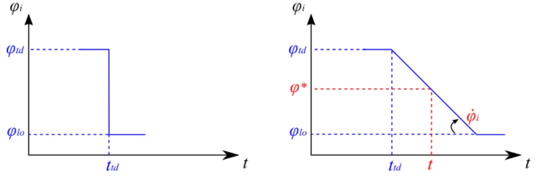
desired angle of a leg with respect to the state of the gait changes according to a desired angular velocity. The change in the desired angle can be represented by a graph as shown Figure 3.6.

Figure 3.6: Trajectory generation system shown for an angle control in a stance phase of a leg. Compared to step change (left), trajectory tracking (right) updates

φ∗_i(t) in each time step with respect to slope or ˙φi.

So instead of changing the desired angle to its full value in a single time step like it is shown on the left graph, we are using the angular velocity as a slope to reach to the desired value. By using this method we can also regulate the amount of torque produced at the actuators. With trajectory tracking, we also eliminate peak torques that can be produced at step changes due to big amounts of diﬀerence between current and desired angles.

The spine actuator is controlled in a similar fashion with its concave and convex poses using the target angles determined by the parameter vector in 3.2. The desired body angle for the concave body pose is computed as

β_s∗(t) = { βs(tf td) + ˙βs(t− tf td) if t− tf td < βcv−βf td ˙ βs βcv otherwise ,

whereas for the convex pose it takes the form

β_s∗(t) = { βs(tf lo)− ˙βs(t− tf lo) if t− tf lo < βcx−βf lo ˙ βs βcx otherwise .

(45)

3.3 Simulation Results

In this section we present simulation experiments comparing our flexible model with the standard stiff-backed model with the bounding gait. In order to make a fair comparison we use optimization methods to find the best performing gait parameters for both models. Subsequently we evaluate the results and compare them to discuss the effects of spinal actuation on the bounding gait.

3.3.1 Conﬁguration and Initialization

We implemented the models described in Section 3.1.3 using the Working Model 2D simulation environment. We used the Kutta-Merson integrator with a ﬁxed time step of 10−3s. To increase the accuracy of the system, the integrator,

as-sembly and overlap error tolerances were chosen to be less than 5× 10−3m. Due

to the limitations of the simulation environment, every test run lasted up to a maximum of 32 seconds.

Table 3.3: System parameters for both bounding models.

Param. Value Param. Value

mbi 10 kg mb 20 kg Ibi 1.3 kg-m2 Ib 3.85 kg-m2 di 0.365 m dsi 0.25 m k 3500 N/m b 55 N m/s l 0.8 m τmax 200 N m µs 0.9 µk 0.8 i∈ {f, b}, f: front, b: back µs, µk : Static and kinetic friction

Physical properties were used for the robot models were inspired from the morphology of a cheetah [10]. It is important to note that both robot models had the same values for these parameters to enable a fair comparison. As the aim of this thesis is to investigate the effects of spinal flexibility on dynamic bounding gaits, we wanted to eliminate other differences between the two robot models. Table 3.3 shows values of each system parameter used in the simulations. The

An actuated flexible spinal mechanism for a bounding quadrupedal robot

a thesis

submitted to the department of computer engineering

and the graduate school of engineering and science

of bilkent university

in partial fulfillment of the requirements

for the degree of

master of science

By

Utku C

¸ ulha

January, 2012

FOR A BOUNDING QUADRUPEDAL ROBOT

¨

OZET

SIC

¸ RAYARAK KOS.AN D ¨

ORT BACAKLI B˙IR ROBOT

˙IC¸˙IN KONTROL ED˙ILEB˙IL˙IR ESNEK BEL OMURGA

MEKAN˙IZMASI

Contents

List of Figures

List of Tables

Introduction

1.1

Dexterous Robotics and Locomotion

1.2

Contributions

1.3

Thesis Organization

Chapter 2

Background

2.1

Locomotion Gaits

2.1.1

Major Gait Types

2.1.2

A Gait Model For Bounding

2.1.3

Legged Robots Capable of Dynamic Bounding

2.2

Existing Work on Flexible Spine Structures

2.3

Gait Optimization Techniques

2.3.1

General Approaches

2.3.2

Nelder-Mead Optimization Algorithm

Chapter 3

Bounding with Flexible Spine

3.1

Planar Robot Models

3.1.1

Standard Model with a Stiﬀ Back

3.1.2

New Model with a Flexible Spine

3.1.3

The Working Model 2D Environment

3.2

Gait Controllers

3.2.1

A New Bounding Gait Model

3.2.2

Design of Bounding Controllers

3.2.3

Local Controllers

3.3

Simulation Results

3.3.1

Conﬁguration and Initialization

_{¸ RAYARAK KOS.AN D ¨}