ANALYSIS OF THE IN-VITRO
NANOPARTICLE-CELL INTERACTIONS VIA SUPPORT VECTOR
REGRESSION MODEL
A THESIS
SUBMITTED TO THE DEPARTMENT OF INDUSTRIAL ENGINEERING AND THE GRADUATE SCHOOL OF ENGINEERING AND SCIENCE
OF BILKENT UNIVERSITY
IN PARTIAL FULFILLMENT OF THE REQUIREMENTS FOR THE DEGREE OF
MASTER OF SCIENCE
By
Nur Muhammed Akbulut
August, 2013
ii
I certify that I have read this thesis and that in my opinion it is fully adequate, in scope and in quality, as a thesis for the degree of Master of Science.
___________________________________ Assoc. Prof. Dr. Savaş Dayanık (Advisor)
I certify that I have read this thesis and that in my opinion it is fully adequate, in scope and in quality, as a thesis for the degree of Master of Science.
___________________________________ Assist. Prof. Dr. Alper Şen
I certify that I have read this thesis and that in my opinion it is fully adequate, in scope and in quality, as a thesis for the degree of Master of Science.
___________________________________ Assist. Prof. Dr. Niyazi Onur Bakır
Approved for the Graduate School of Engineering and Science:
___________________________________ Prof. Dr. Levent Onural
iii
ABSTRACT
ANALYSIS OF THE IN-VITRO NANOPARTICLE-CELL
INTERACTIONS VIA SUPPORT VECTOR REGRESSION
MODEL
Nur Muhammed Akbulut M.S. in Industrial Engineering Supervisor: Prof. Dr. Savaş Dayanık
Co-Supervisor: Assoc. Prof. Dr. İhsan Sabuncuoğlu August 26, 2013
In this research a Support Vector Regression model is developed to understand the nanoparticle (NP)-cell interactions and to predict the cellular uptake rate of the nanoparticles, which is the rate of NPs adhered to the cell surface or entered into the cell. Examination of nanoparticle-cell interaction is important for developing targeted drug delivery systems and cell-level detection and treatment of diseases. Cellular uptake rate of NPs depends on NP type, size, shape, surface charge, concentration and incubation time. Conducting numerous experiments on the combinations of those variables to understand NP-cell interaction is impractical. Hence, a mathematical model of the cellular uptake rate will therefore be useful. The data for this study are obtained from in-vitro NP-healthy cell experiments conducted by a Nano-Medicine Research Center in Turkey. The proposed support vector regression model predicts the cellular uptake rate of nanoparticles with respect to incubation time given the size, charge and concentration properties of NPs.
Keywords: Nano-medicine, targeted drug delivery, nanoparticle uptake rate, support
iv
ÖZET
DESTEK VEKTÖR REGRESYON MODELİ İLE
İN-VİTRO NANOPARTİKÜL-HÜCRE
ETKİLEŞİMLERİNİN MODELLENMESİ
Nur Muhammed Akbulut Endüstri Mühendisliği, Yüksek Lisans Tez Yöneticisi: Doç. Dr. Savaş Dayanık Yardımcı Tez Yöneticisi: Prof. Dr. İhsan Sabuncuoğlu
Ağustos, 2013
Bu araştırmada, Destek Vektör Regresyon (DVR) yöntemi ile nanopartikül-hücre etkileşimini inceleyen ve hücreye tutunan yani hücre yüzeyine yapışan veya hücre içine alınan nanopartikül (NP) oranını tahmin eden bir model geliştirilmiştir. Güdümlü ilaç dağıtımı sistemleri ve hücre seviyesinde hastalıkların tanı ve tedavileri için NP-hücre etkileşimini analiz etmek önemli bir araştırma konusudur. Nanopartiküllerin hücreye bağlanma oranları NP tipi, boyutu, şekli, yüzey yükü, yoğunluğu ve zaman değişkenlerine bağlı olarak farklılık göstermektedir. NP-hücre ilişkisini açıklamak için bu değişkenlerin binlerce varyasyonunu deneylerle test etmek pratik değildir. Bu yüzden, farklı varyasyonlar için nanopartiküllerin hücreye tutunma oranlarını matematiksel bir model yardımı ile tahmin etmek önemli bir çalışmadır. Çalışma için kullanılan veri seti Türkiye'de bir Nano-Tıp Araştırma Merkezi tarafından yapılan in-vitro NP-hücre etkileşimi deneyleri sonucunda elde edilmiştir. Geliştirilen DVR modeli, nanopartiküllerin verilen büyüklük, yoğunluk, yüzey yükü özelliklerini girdi olarak alarak; nanopartiküllerin hücreye tutunma oranlarını zamana bağlı olarak tahmin etmektedir.
Anahtar Sözcükler: Nano-tıp, güdümlü ilaç dağılımı, hücre içine nanopartikül alım
v
Acknowledgement
I would like to express my gratitude to my supervisors Assoc. Prof. Dayanık and Prof. Sabuncuoğlu for the useful comments, remarks and engagement through the learning process of this master thesis. Furthermore I would like to thank Assoc. Prof. Budak for introducing us to the topic as well for the support on the way.
I am also grateful to TÜBİTAK for providing the financial support.
I would also like to thank my parents, brothers and sister. They were always supporting me and encouraging me with their best wishes.
Finally, I would like to thank my wife, Elif Akbulut. She was always there cheering me up and stood by me through the good times and bad.
vi
Contents
1 Introduction 1
2 Literature Review 4
3 Background on Support Vector Regression 8
4 Experimental Procedure of Proposed Study 18
5 Proposed SVR Model 21
5.1 Proposed Model for PMMA NPs 25
5.2 Proposed Model for Silica NPs 31
5.3 Proposed Model for PLA NPs 39
6 Comparison and Discussions 44
7 Conclusion 57
vii
List of Figures
Figure 1. ε-Loss function and Slack Variable ξ……….. 9
Figure 2. PMMA 50nm predictions……… 27 Figure 3. PMMA 100nm predictions……….. 28 Figure 4. t-score of size difference ((-) Charged PMMA NPs, 0.001 Concentration)…… 30 Figure 5. t-score of size difference ((-) Charged PMMA NPs, 0.01 Concentration)…….. 30 Figure 6. Silica 50nm predictions ……….. 32 Figure 7. Silica 100nm predictions………. 33 Figure 8. t-score of size difference ((-) Charged Silica NPs, 0.001 Concentration) for
Silica I………. 35
Figure 9. t-score of size difference ((-) Charged Silica NPs, 0.001 Concentration) for Silica II……… 35 Figure 10. t-score of size difference ((-) Charged Silica NPs, 0.01 Concentration) for
Silica I………. 36
Figure 11. t-score of size difference ((-) Charged Silica NPs, 0.01 Concentration) for
Silica II……… 36 Figure 12. t-score of size difference ((+) Charged Silica NPs, 0.001 Concentration) for
Silica I………. 37
Figure 13. t-score of size difference ((+) Charged Silica II NPs, 0.001 Concentration)
viii
Figure 14. t-score of size difference ((+) Charged Silica NPs, 0.01 Concentration) for
Silica I………. 38
Figure 15. t-score of size difference ((+) Charged Silica NPs, 0.01 Concentration) for Silica II……… 38
Figure 16. PLA predictions………. 40
Figure 17. t-score of concentration difference ((-) Charged PLA NPs)……….. 41
Figure 18. t-score of concentration difference ((+) Charged PLA NPs)………. 42
Figure 19. t-score of charge difference (0.01 Concentration PLA NPs)………. 42
Figure 20. t-score of charge difference (0.001 Concentration PLA NPs)………... 43
Figure 21. PLA predictions of our model and Cenk’s model………. 47
Figure 22. PLA predictions of our model and Dogruoz’s model……… 48
Figure 23. PMMA 50 nm predictions of our model and Cenk’s model………. 49
Figure 24. PMMA 100 nm predictions of our model and Cenk’s model………... 50
Figure 25. PMMA 50 nm predictions of our model and Dogruoz’s model……… 51
Figure 26. PMMA 100 nm predictions of our model and Dogruoz’s model……….. 52
Figure 27. Silica 50 nm predictions of our model and Cenk’s model……… 53
Figure 28. Silica 100 nm predictions of our model and Cenk’s model……….. 54
ix
x
List of Tables
Table 1. Input variables……….. 22
Table 2. Experimental groups of PMMA and Silica nanoparticles………. 25
Table 3. Model parameters for PMMA NPs……… 25
Table 4. Standard deviation of mean uptake rates for PMMA……… 26
Table 5. Silica I and Silica II model parameters for Silica NPs……….. 31
Table 6. Standard deviation of mean uptake rates for Silica………... 34
Table 7. Experimental groups of PLA nanoparticles………... 39
Table 8. Model parameters for PLA NPs……… 39
1
Chapter 1
Introduction
Cancer causes the body cells become abnormal and divide and grow uncontrollably. Cancer cells may invade any tissue of the body and may spread through the blood or lymphatic system to other parts of the body. If this spread is not controlled, it can result in death. According to the World Cancer Report of The International Agency for Research on Cancer 7.6 million which is nearly one in eight of all deaths in the world is caused by cancer in 2008. According to the report this number will almost be doubled in 2030 [1]. National Cancer Institute’s Surveillance Epidemiology and End Results (SEER) program claimed that there are 12.5 million people who suffer from cancer only in United States by 2009 [2].
Therefore, researchers work hard to find effective ways of diagnosis and treatment of cancer. Surgical operations, radiation and chemotherapy are the current treatment methods for cancer. However, those methods have severe side effects on the body. Those methods often harm healthy cells and cause toxicity. Cancer cells may also reappear in the body after the treatment.
2
Nanotechnology is an emerging and evolving technology and there have been an interest in using it in cancer research. Targeted drug delivery system is one of the most fundamental research areas related to both nanotechnology and biotechnology [3]. Targeted drug delivery is a method of delivering medication to the body in a manner such that the concentration of the medication in the diseased tissues is higher than that in the healthy cells. Current research focuses on using nanoparticles with pharmacological agents to kill cancer cells in a targeted drug delivery system. Since those studies are conducted at cell-level, a careful investigation of nanoparticle (NP)-cell interaction and (NP)-cellular uptake efficiency, which is defined as the rate of NPs adhered to the surfaces of the cells or entered into the cells is very important for targeted drug delivery.
Cellular uptake efficiency is affected by size, type (chemical structure), shape, surface charge and the concentration of NPs. It is impractical or too costly to conduct all of the possible configurations of those variables in laboratory conditions. Therefore, this thesis aims to develop a prediction model based on data from in-vitro NP-cell interaction experiments. The proposed model predicts the cellular uptake rate of NPs on different combinations. In this study, the prediction model is developed by using Support Vector Regression (SVR) technique. SVR approach is preferred because it is a powerful tool to model non-linear complex systems. Since SVR presents a solution by means of small subset of training data, it also gives enormous computational advantages.
3
Data for this study are obtained from in-vitro experiments that are conducted by a Nano-Medicine Research Center in Turkey. Silica, polymethyl methacrylate (PMMA) and polylactic acid (PLA) are the types of nanoparticles used in those experiments. Data include the uptake rate of nanoparticles for different combinations of NP size, charge and concentration at particular times. Then we propose a prediction model for 48 hours incubation period by using SVR method on those data.
The primary contribution of this study is a prediction method for the uptake rate of NPs in the nanomedicine field. The second contribution is a thorough implementation of SVR for statistics field based on real data.
The remainder of the thesis is organised as follows: The related literature is reviewed in Chapter 2. Chapter 3 introduces Support Vector Regression. The design of the experiments is discussed in Chapter 4. The proposed models and results of computational study are presented in Chapter 5. Chapter 6 compares and discusses the results of our model with those of the previous studies. Finally, Chapter 7 concludes the thesis.
4
Chapter 2
Literature Review
There are numerous experimental studies on nanoparticle-cell interaction and cellular uptake rate of nanoparticles in the literature. In those studies, effects of some characteristics of NPs such as chemical structure, size, surface charge, concentration and incubation time on the interaction with cells are explored. Although those studies give information about the effects of some NP characteristics on cell interactions, mathematical models built on those findings are very rare.
Chitrani et al. [4] investigated the influence of different size and shape of colloidal gold nanoparticles for different incubation times over intracellular uptake inside mammalian cells. In their study, spherical NPs with diameters of 14, 30, 50, 74 and 100 nm and rod-shaped NPs with dimensions 40x14 nm and 74x14 nm are used. They conclude that, uptake rate rapidly increases for the first 2 hours, and then becomes steady at 4-7 hours for different sizes. Their experiments also show that uptake rate for 50 nm NPs is higher than that for other sizes. Shape also has impact on uptake rate. They demonstrated that more spherical NPs are taken into the cell than the rod-shaped NPs. Therefore, their research demonstrates that desired cellular
5
uptake rate may be achievable by adjusting the size and shape of the NPs. However, the findings of their study are observational and did not lead to a mathematical model of the NP-cell interaction. Davda and Labhasetwar [5] examine the NP-endothelial cell interaction. They observe that the cellular uptake of nanoparticles depends on the incubation time and uptake rate increases with increase in the concentration of nanoparticles in the medium. Their study sheds light on the biocompability of the NPs with cells. According to their study concentration of NPs have impact on uptake rate. Peetla and Labhasetwar [6] investigate the interaction between endothelial cell membrane and nanoparticles. 20 nm and 60 nm sized polystyrene NPs of different surface charges are used to analyze the changes in the membrane’s surface pressure. The results show that positively charged 60 nm NPs increase surface pressure while neutral NPs reduced surface pressure and negatively charged NPs of the same size have no effect. However, 20 nm NPs have greater interactions with the cell for all surface charges. Their study does not provide a mathematical model but it is significant to understand how the characterizations of nanoparticles affect the interaction with cells. In all those studies, NP-cell interactions are examined by only physical experimentations for only two or three variables, without using a proper mathematical model. Therefore, they are not capable of predicting cellular uptake rate without conducting the experiments.
Lin et al. [7] investigate the interactions between different surface charge densities and signs of gold nanoparticles and cell membranes by developing coarse-grained molecular dynamics simulation model. They reach the conclusion that
6
positively charged nanoparticles adhere to cell membrane more than negatively charged nanoparticles and level of penetration increases as the charge density of NPs increases. They show that the adhesion and penetration level can be controlled by adjusting the surface charges and densities.
Boso et al. [8] provides the only mathematical model on NP-cell interaction in the literature. They seek to determine the optimum NP diameter that maximizes the NPs adhered to the diseased blood vessel walls. They conducted a parallel plate flow chamber in vitro experiments with spherical polystyrene NPs. They develop an artificial neural network model to predict the number of NPs adhering per unit area as a function of shear rate and NP diameter. They show that an optimal NP diameter exists that maximizes the number of NPs adhere to the vessel walls. This study considers the effects of only NP size and wall shear rate on the NP accumulation, but other properties of NPs such as type, shape, charge and concentration are not considered. Albeit the study is limited in terms of investigating factors that affect NP-cell interactions, this study contains a mathematical model and demonstrate that accurate prediction can be used effectively to minimize the number of experiments needed which is the motivation for this study.
Cenk [9] and Dogruoz [10] studies have recently proposed models of NP-cell interactions. They investigate the effects of NP size, surface charge, concentration, and chemical structure on NP-cell interactions. Those studies and our study use the same data to build prediction models for the cellular uptake rate of NPs. However, their modeling approaches are different. Cenk [9] develops an artificial neural
7
network model whereas Dogruoz [10] uses a statistical mixed model approach. Chapter 6 compares the results of our study with those of Cenk [9] and Dogruoz [10].
SVR was not studied to investigate the NP-cell interactions in the past. However, it is applied to many real-world problems successfully. When it is compared to other modeling tools, SVR generalization ability shows either similar or significantly better performance than competing methods in most of the cases [11]. Hence, SVR is an appropriate tool to examine NP-cell interaction. This study will be helpful to understand the interaction between nanoparticles and cells for the nanomedicine and targeted drug delivery studies. A new application area for SVR will contribute to the statistics literature.
8
Chapter 3
Background on Support Vector Regression
Support Vector Regression (SVR) is based on statistical learning theory and has been developed by Vapnik [12]. This new technique provides an efficient and novel approach to improve generalization performance. SVR achieves good generalization ability by adopting a structural risk minimization principle. Structural risk minimization (SRM) seeks to minimize an upper bound on the generalization error rather than minimize the empirical error (empirical risk minimization (ERM)) focused in by many of the other modeling techniques. It has been show that SRM is superior to ERM principle employed by other techniques such as Artificial Neural Networks. SVR is trained with optimization of a quadratic cost function, which guarantees the attainment of a global minimum.
The construction of SVR to estimate a regression function is based on three distinct characteristics of SVR. Firstly, SVR estimate the regression function using a set of linear functions that are defined in a high dimensional space. Secondly, SVR defines the regression estimation as the problem of risk minimization with respect to the Vapnik’s ε-insensitive loss function. Thirdly, SVR minimizes the risk function
9
consisting of the empirical error and a regularization term which is derived from the SRM principle.
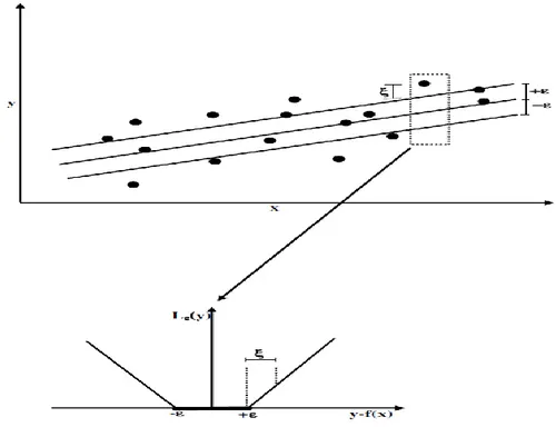
The ε-insensitive loss function can be defined as:
if ( )
( )
( ) , otherwise (3.1)
This loss function defines an ε tube (Figure 1) which means, if the predicted value is inside the tube the loss is zero; if the predicted value is outside the tube the loss is the magnitude of the difference between the predicted value and data point and the radius, ε.
10
Assume that the training data set consists of sample {( ) ( )} where is the input and is the output. The problem is to choose a function that predicts as closely as possible with a precision of .
Now, let us assume a linear predictor.
( ) ( ) (3.2)
where is an adjustable weight vector and and are the n-dimensional and 1-dimensional vector space, respectively.
The main purpose of SVR is to find a function ( ) that gives at most -deviation from (actual output) and at the same time as flat as possible. Flatness in (3.2) can be achieved by seeking small . One way of doing this is by minimizing which is the Euclidean norm of [13]. Thus, convex optimization problem is to
minimize | |
subject to
( )
( ) (3.3)
The best regression line is found by solving
| | ∑( )
11
( )
( )
and (3.4)
The term | | is called the regularized term. The second term ∑ ( ), is the so called empirical error (risk), which is measured by the ε-insensitive loss function in (3.1). is the regularization constant determining the trade-off between
empirical risk and regularized term. In the error term, predictions which are deviating by less than or more than are taken into account by slack variables and , respectively (Figure 1). Value of should be determined by the user. One should note that is not the final desired prediction of the model. It is a characteristic of the
prediction error penalty. In addition to , the penalty weight should also be optimally chosen by the user. If it is chosen too small, the best result is determined by the size of the regression weights. On the other hand, if it is chosen too large, the best solution will be determined by minimizing the empirical error.
In order to solve the problem in (3.4) the following Lagrangian function is constructed.
12 ( ) | | ∑( ) ∑ ( ) ∑ ( ) ∑( ) (3.5) where is the Lagrangian and are the Lagrangian multipliers. It follows from the saddle point condition that partial derivatives of with respect to primary variables have to vanish for optimality.
↔ ∑ ( ), ↔ ∑ ∑ , ↔ ∑ ∑ ( ),
↔ ∑ ∑ ( ) , (3.6) Substituting (3.6) into (3.5) yields the following dual optimization problem.
∑( ) ∑ ( ) ∑ ∑( )( )( ) subject to
13 ∑ ∑ , (3.7)
The coefficients , are determined by solving (3.7). Some of these multipliers ( , ) will be zero. The corresponding training points are irrelevant for
the final solution. The training objects with non-zero Lagrangian multipliers are called support vectors. Support vectors are the objects where prediction errors are larger than ± . Then equation (3.2) can be written as;
( ) ∑ ( )( ) where ( ) (3.8) where denotes the collection of support vectors.
In most problems linear regression is not appropriate. When it is not, the input data must be mapped into a high dimensional feature space where linear regression is performed through some nonlinear mapping [14]. Then is replaced by the feature space representation, ( ) in the above optimization problem. Therefore; (3.7) can
be written as kkkkkkkkkkkkkkkkkkkkkkkkkkkkkkkkkkkkkkkkkkkkkkkkkkkkkkkk ∑( ) ∑ ( ) ∑ ∑( )( )( ( ) ( ))
14 subject to ∑ ∑ (3.9)
To reduce the computational load, kernel function defined by
( ) ( ) ( )
Cortes and Vapnik [15] introduced.
The optimization problem can be written as
∑( ) ∑ ( ) ∑ ∑( )( ) ( ) subject to ∑ ∑ (3.10)
and the regression function can be written as ( ) ∑ ( ) ( )
15
SVR model provides only an estimated target value. However, we also want to calculate a prediction interval. In order to find prediction intervals, we use the well-functioning approach of Lin et al. [16] as we explain now.
We are given a set of training data {( ) ( )} . We suppose that
( ) , (3.12)
where and are independent and identically distributed random noises.
Given a test data , the distribution of given and is ( ). This allows one to construct a prediction interval ( ) such that with a pre-specified probability. If we denote ̂( ) as the estimated function based on , then ( ) ̂( ) is the out-of-sample residuals (prediction error) and is equivalent to ̂( ).
It is proposed to model the distribution of based on a set of out-of-sample residuals { } using training data . The ’s are generated by first conducting a k-fold cross validation to get ̂ , and then setting ̂( ) for ( ) in the jth fold. It is conceptually clear that the distribution of ’s may
resemble that of the prediction error .
Lin et al. [16] propose to model by zero-mean Gaussian and Laplace, or equivalently, model the conditional distribution of given ̂( ) by Gaussian and Laplace with mean ̂( ).
16
To obtain the fitted curves using Laplace and Gaussian distributions, we first express the density functions of zero-mean Laplace and Gaussian with scale parameter , Laplace ( ) (3.13) Gaussian ( ) √ (3.14)
Next, assuming that are independent, we can estimate the scale parameter by maximizing the likelihood. For Laplace, the maximum likelihood estimate is,
∑
(3.15)
and for Gaussian,
∑ (3.16)
Then we obtain the fitted curves by plugging these estimates into (3.13) and (3.14).
After then (1-2s)100% prediction interval for is ( ̂( ) ̂( ) ) where is the upper sth percentile of the corresponding probability distribution of .
For example, a Laplace with ( ) as in (3.13) has ( ) and resulting prediction interval for is
17
A Gaussian with ( ) defined in (3.12) has ( ) where ( ) is the
cumulative density function of Gaussian distribution, and the prediction interval for is
( ( ) ( )) (3.18)
In order to decide either Laplace or Gaussian for the distribution of will be used, one should investigate ’s. Visual detection of the histogram of ’s and fitted Laplace and Gaussian models, can be helpful to decide which model captures ’s
better. However, this method can be subjective and may not be efficient for some cases. We refer the interested reader to Lin et al [16] between Gaussian or Laplace distribution.
18
Chapter 4
Experimental Procedure of Proposed Study
Expertise and advanced technology are used for the synthesis of nanoparticles to be used for diagnostics and targeted drug delivery at cell-level. In this process, synthesized NPs can be characterized according to targeted cell/tissue in order to find and enter in or adhere to targeted cell/tissue. Therapeutic agents are inserted in chemically or immunologically characterized nanoparticles to treat cells. Advanced technology enables us to place both therapeutic and diagnostic contrast agents together. This method, called as “theragnostic” allows cell-level treatment and diagnosis simultaneously. NPs that are used for theragnostic purposes should be designed properly. There are five main variables of NPs for the design of a theragnostic purpose: type (chemical structure), shape, surface charge and concentration of NP solution.
The data set for the SVR model is obtained from in-vitro nanoparticle-cell interaction experiments conducted by Nanomedicine Research Center. Three types of NPs were used for in-vitro nanoparticles-healthy cell interaction experiments: polymethyl methacrylate (PMMA), silica and polylactic acid (PLA). All of those NPs were sphere-shaped. Two different diameter sizes (50 nm and 100 nm) were
19
used for silica and PMMA nanoparticles, and only one diameter size (250 nm) was used for PLA nanoparticles. For each type of nanoparticles two different surface charges were selected. For each type of nanoparticle, two different concentrations of NP solutions (0,001 mg/l and 0, 01 mg/l) were prepared for the experiments. Cellular uptake rate of NPs was measured at some specific times.
In experiments, "3T3 Swiss albino Mouse Fibroblast" type of healthy cell set was used to interact with nanoparticles. Cells were incubated in medium containing 10% FBS, 2 mm L-glutamine, 100 IU / ml penicillin and 100 mg / ml streptomycin at 37 °C with 5% CO2. After incubation, proliferating cells in the culture flask were passaged using PBS and trypsin-EDTA solution. Then, cells incubated for 24 hours were counted and placed on 96-well cell culture plates. After then, prepared solutions of NPs were added to those cell culture plates.
Cells and nanoparticles interacted in in-vitro experiments by using micromanipulation systems in the labs established as a ''clean room'' principle. Transmission electron microscopy, spectrophotometric measurement methods, and confocal microscopy were used in order to observe NP-cell interactions and to obtain the data.
There were 20 different configurations of NPs for these experiments. For Silica and PMMA NPs, 8 different configurations (50 or 100 nm, positive or negatively charged, 0.001 or 0.01 mg/l concentration); for PLA NPs 4 different configurations (250 nm, positive or negatively charged, 0.001 or 0.01 mg/l concentration) were created. Experiments were repeated six times for each configuration. In order to
20
determine NP-cell interaction behavior by time cell cultures were observed at 3, 6, 12, 24, 36, and 48 hours of incubation. In order to find the cellular uptake efficiency of nanoparticles, the following steps were applied. Immediately after the incubation period, the number NP removed from the environment is calculated by washing the solution. Subtracting this number from the initially applied number of NPs gives the number of NPs adhered to the cell surface or penetrated into the cell. Then, by dividing this number to the initial number of NPs cellular uptake efficiency is found.
After conducting the above experiments, for 8 different configurations of Silica NPs, the experiments were repeated. In those experiments, measurements were taken at 1.5, 4, 9, 18, 30 and 42 hour of incubation in order to observe the process in time intervals of the first replication. Also, for two configurations of PMMA NPs (size of 50 and 100 nm with concentration of 0.001 mg/l and positive surface charge), the experiments were repeated as in the first experiment set to check for the consistency of the results of the first replication. The raw data is graphically illustrated in Appendix.
21
Chapter 5
Proposed Model
In this research, we aim to model the cellular uptake rate of NPs of different qualities over time. For this aim, we use Support Vector Regression model, which is explained in Chapter 3. The proposed model is implemented in Matlab Programming Language.
We fit a model for Silica, PMMA and PLA nanoparticles. Due to their different chemical structures, their interactions with cells show very different behavior from each other. The values of the input variables used in the study are given in Table 1.
In order to apply SVR model on these data, surface charge of NPs is converted to numerical values. Before applying the model, data are scaled between 0 and 1 to increase the efficiency of SVR model.
22 Table 1:Input variables
1. Input Variable Value
2. Types of NPs PMMA, Silica, PLA
3. Diameter size of NPs 50 nm and 100 nm for PMMA and Silica 250 nm for PLA 4. Surface charge of NPs Positive (1) and Negative (0)
5. Concentrations of NPs 0,001 - 0,01 mg/l
6. Incubation time 0,3, 6, 12, 24, 36, 48 hours for PMMA, Silica and PLA 0,1.5, 4, 9, 18, 30, 42 hours for silica
Output of the proposed SVR model is cellular uptake efficiency of NPs which is the only dependent variable of the experiments. Cellular uptake efficiency is the ratio of number of NPs over the cell surface or inside the cells to the initial number of NPs and calculated as follows:
Note that at time zero, for all type of NPs the cellular uptake rate is zero. Hence, the proposed SVR model should guarantee this property. Therefore, we use a modified version of SVR called weighted SVR that will satisfy the uptake rate will be zero at time zero [17].
23
Recall the objective function of (3.4). Instead of using a common penalty term C, we use a weight factor si for C for each data point i. Then we solve the
following the quadratic problem, applying the same steps as in Chapter 3.
| | ∑ ( )
subject to ( )
( )
and (5.1)
By the help of this new formulation; cellular uptake prediction for time zero can be within Ɛ neighborhood of zero. We can achieve this result by making for data points where time is zero and for other data points.
To construct the proposed SVR models for PMMA, Silica and PLA nanoparticles, first we need to determine the kernel that will be used for mapping data to a higher dimensional space in order to get nonlinear regression model. Dibike et al. [18] presented some results showing that Radial Basis Function (RBF) is the best kernel function to be used in SVM models. We use Gaussian Radial Basis Function (RBF) as kernel function.
( ) ( )
where, is the parameter of the function and should be determined by the user. Smaller values of give a smoother regression functions.
24
We should also determine the value of penalty term ’s and . The
selection of the user-defined parameters has significant effects on the performance of the regression function. The best parameter set ( , , ) for a given problem is unknown. In the first step of this research, mean square error (MSE) is used as performance measure for different combinations of parameters ( , , ). However, the best parameter set selected according to MSE criterion resulted in overfits the data. Since SVR is problem and data dependent, selection of the parameter values should be based on expert opinion. Our problem is related to living organisms and has complex structure. Moreover, data are obtained only for seven distinct hours over a 48-hours interval. Therefore, for each type of nanoparticles we made search a grid of ( , , ) 11*11*11=1331 models are presented to the choice of the experts. The best parameter sets were chosen based on the expert opinion.
In Sections 5.1, 5.2 and 5.3 the proposed models for PMMA, Silica and PLA are given, respectively. In all given models, it is seen that there is a rapid entry of NPs into to the cell at the beginning of incubation periods. After some time, uptake rate decreases and then increases again and continues to fluctuate in this manner. Although general behavior looks similar, the overall behavior and uptake rates change with the characteristics of NPs.
25
5.1. Proposed Model and Results for PMMA NP
For PMMA NP experiments, measurements were taken at 3, 6, 12, 24, 36, 48 hours of incubation. For each experiment sets, there are 8 different combinations of PMMA NPs as in Table 2. The values of the parameters for SVR models were determined by expert opinions and are tabulated below.
Table 2: Experimental groups of PMMA and Silica nanoparticles
Group Size Charge Density
1 50 nm (+) 0.001 mg/l 2 50 nm (+) 0.01 mg/l 3 50 nm (-) 0.001 mg/l 4 50 nm (-) 0.01 mg/l 5 100 nm (+) 0.001 mg/l 6 100 nm (+) 0.01 mg/l 7 100 nm (-) 0.001 mg/l 8 100 nm (-) 0.01 mg/l
Table 3: Model parameters for PMMA NPs
Parameter ( )
Value 71 71000 0.001 1.347
Figures 2 and 3 show the hourly prediction values of the proposed models for PMMA NPs. Mean uptake rates for each configuration over 48 hours and their standard deviations are given in Table 4. Model gives a good fit with mean square error (MSE) 0.00244 and R-squared value 0.961. Results mostly show that negatively charged NPs have smaller standard deviations when size and
26
concentration are constant. Positively charged NPs show large fluctuations for PMMA NPs. Moreover, when sizes are same, high concentration (1/100 mg/l) has smaller standard deviations than low concentration (1/1000 mg/l) for negatively charged NPs.
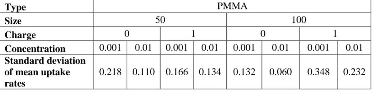
Table 4: Standard deviation of mean uptake rates for PMMA
Type PMMA Size 50 100 Charge 0 1 0 1 Concentration 0.001 0.01 0.001 0.01 0.001 0.01 0.001 0.01 Standard deviation of mean uptake rates 0.218 0.110 0.166 0.134 0.132 0.060 0.348 0.232
In order to understand the effect of 50 nm and 100 nm sizes for negatively charged PMMA, hypothesis testing for the difference between two means is applied. Therefore, we made 50 simulation runs that depend on our prediction model. Mean and standard deviations of 50 samples are calculated for each hour between 0 and 48. By the central limit theorem, since sample size is greater than 40, each sample is independent simple random sampling with approximately normal distribution. We utilized from two-sample t-test to understand whether there is a significant difference between means or not. The hypothesis is stated as follows:
Null hypothesis: effects of 50 nm and 100 nm are same H0: μ1 = μ2
27 Data points Predictions 95% Prediction interval Figure 2: PMMA 50nm predictions
28 Data points Predictions 95% Prediction interval Figure 3: PMMA 100nm predictions
29
Significance level is 0.05 for this analysis and degrees of freedom is n-1=49. t-score test statistic is calculated as ( ) where and are the means of sample 1 and 2, is the hypothesized difference between population means and is the
standard error. Standard error is computed as √( ) ( ) where is the standard deviation of sample 1, is the standard deviation of sample 2, and is the size of sample 1, and is the size of sample 2.
We have a two tailed test; P(t<-2.01)=0.025 and P(t>2.01)=0.025 and we reject null hypothesis when P-value is less than the significance level. Null hypothesis is rejected when t-score is either smaller than -2.01 or greater than 2.01.
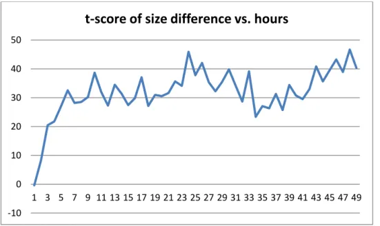
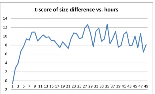
Figures 4 and 5 show the hourly t-score values for negatively charged PMMA NPs. In low concentration case, P-value is less than the significance level only for a small portion of time. Therefore, there is no clear difference between 50 nm and 100 nm NPs. In high concentration case, t-score is always more than 2.01, which shows that 50 nm NPs lead to higher uptake rate. When we consider the results for a targeted delivery system, it is reasonable to prefer negatively charged, 50 nm and high concentration of PMMA NPs since they result in high uptake rate show more stable behavior.
30
Figure 4: t-score of size difference ((-) Charged PMMA NPs, 0.001 Concentration)
Figure 5: t-score of size difference ((-) Charged PMMA NPs, 0.01 Concentration) -50 -40 -30 -20 -10 0 10 20 30 40 50 1 3 5 7 9 11 13 15 17 19 21 23 25 27 29 31 33 35 37 39 41 43 45 47 49
t-score of size difference vs. hours
-10 0 10 20 30 40 50 1 3 5 7 9 11 13 15 17 19 21 23 25 27 29 31 33 35 37 39 41 43 45 47 49
31
5.2. Proposed Model and Results for Silica NP
For Silica nanoparticles, the experiments were made at two distinct times with different incubation periods. In the first series of experiments, measurements were taken at 3, 6, 12, 24, 36, 48 hours of incubation. In the second series of experiments, measurements were taken at 1.5, 4, 9, 18, 30, 42 hours of incubation. For each experiment sets, there are 8 different combinations of Silica NPs as PMMA NPs given in Table 2.
Since there are two different data sets obtained at different experiment series, we fit two different SVR model for Silica NPs and named as Silica I and Silica II models. The values of the parameters for SVR models were determined by expert opinions and are tabulated below.
Table 5: Silica I and Silica II model parameters for Silica NPs
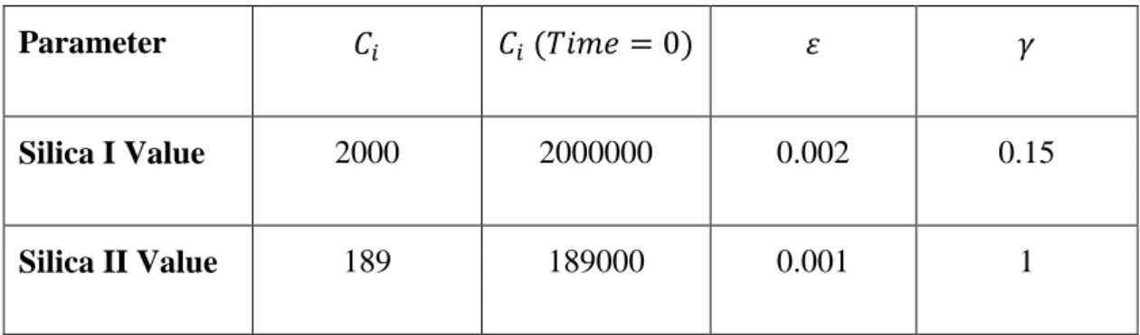
Parameter ( )
Silica I Value 2000 2000000 0.002 0.15
Silica II Value 189 189000 0.001 1
Figure 6 and 7 show the hourly prediction values of the proposed models for Silica NPs. Silica I model has MSE=0.01 and R-squared value=0.88 whereas Silica II model has MSE=0.008 and R-squared value=0.915 as performance indicators of models.
32
Data points 1st set Predictions Silica I 95% Prediction interval Data points 2nd set Predictions Silica II 95% Prediction interval Figure 6: Silica 50nm predictions
33
Data points 1st set Predictions Silica I 95% Prediction interval Data points 2nd set Predictions Silica II 95% Prediction interval Figure 7: Silica 100nm predictions
34
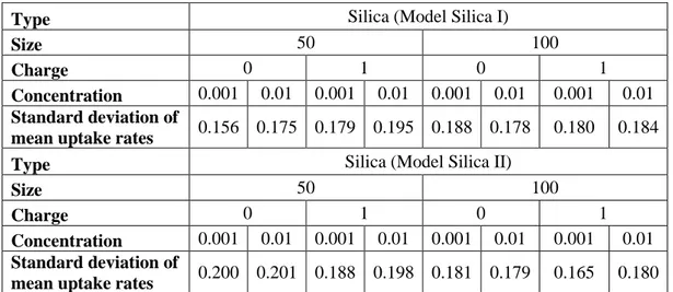
Table 6: Standard deviation of mean uptake rates for Silica
Type Silica (Model Silica I)
Size 50 100
Charge 0 1 0 1
Concentration 0.001 0.01 0.001 0.01 0.001 0.01 0.001 0.01
Standard deviation of
mean uptake rates 0.156 0.175 0.179 0.195 0.188 0.178 0.180 0.184 Type Silica (Model Silica II)
Size 50 100
Charge 0 1 0 1
Concentration 0.001 0.01 0.001 0.01 0.001 0.01 0.001 0.01
Standard deviation of
mean uptake rates 0.200 0.201 0.188 0.198 0.181 0.179 0.165 0.180
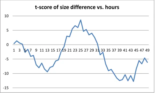
Mean uptake rates for each configuration over 48 hours and their standard deviations are given in table above. Silica NPs have higher uptake rates than PMMA NPs in general. We applied two-sample t-test for difference of 50 nm and 100 nm sizes of Silica NPs. Same procedure is followed as conducted for PMMA NPs. For (-) charged NPs we fail to reject null hypothesis for all 0-48 hours interval since t-scores are sometimes within the range (-2.01, 2.01). However, at other times t-t-scores are mostly less than -2.01 for both models. This shows that although we fail to reject the null hypothesis for whole interval, 100 nm size lead to high uptake rate for most of the time. Same deduction is valid for the (+) charged NPs in 0.001 concentration, because we fail to reject the null test for some parts of the interval and for other parts of the interval score is less than -2.01. For (+) charged NPs in 0.01 concentration, t-scores are always greater than 2.01 for Silica II model and mostly greater than 2.01 for Silica I model. This means that 50 nm size lead to higher uptake rate for (+)
35
charged, high concentration Silica NPs. It is also seen that uptake rates are greater for high concentration than low concentration with constant NP size and charge.
Figure 8: t-score of size difference ((-) Charged Silica NPs, 0.001 Concentration) for Silica I
Figure 9: t-score of size difference ((-) Charged Silica NPs, 0.001 Concentration) for Silica II -14 -12 -10 -8 -6 -4 -2 0 2 4 1 3 5 7 9 11 13 15 17 19 21 23 25 27 29 31 33 35 37 39 41 43 45 47 49
t-score of size difference vs. hours
-15 -10 -5 0 5 10 1 3 5 7 9 11 13 15 17 19 21 23 25 27 29 31 33 35 37 39 41 43 45 47 49
36
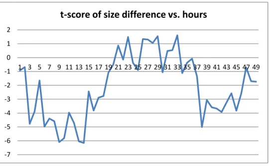
Figure 10: t-score of size difference ((-) Charged Silica NPs, 0.01 Concentration) for Silica I
Figure 11: t-score of size difference ((-) Charged Silica NPs, 0.01 Concentration) for Silica II -7 -6 -5 -4 -3 -2 -1 0 1 2 1 3 5 7 9 11 13 15 17 19 21 23 25 27 29 31 33 35 37 39 41 43 45 47 49
t-score of size difference vs. hours
-35 -30 -25 -20 -15 -10 -5 0 5 1 3 5 7 9 11 13 15 17 19 21 23 25 27 29 31 33 35 37 39 41 43 45 47 49
37
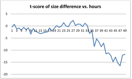
Figure 12: t-score of size difference ((+) Charged Silica NPs, 0.001 Concentration) for Silica I
Figure 13: t-score of size difference ((+) Charged Silica II NPs, 0.001 Concentration) for Silica II -9 -8 -7 -6 -5 -4 -3 -2 -1 0 1 2 1 3 5 7 9 11 13 15 17 19 21 23 25 27 29 31 33 35 37 39 41 43 45 47 49
t-score of size difference vs. hours
-20 -15 -10 -5 0 5 1 3 5 7 9 11 13 15 17 19 21 23 25 27 29 31 33 35 37 39 41 43 45 47 49
38
Figure 14: t-score of size difference ((+) Charged Silica NPs, 0.01 Concentration) for Silica I
Figure 15: t-score of size difference ((+) Charged Silica NPs, 0.01 Concentration) for Silica II -6 -4 -2 0 2 4 6 8 10 12 14 1 3 5 7 9 11 13 15 17 19 21 23 25 27 29 31 33 35 37 39 41 43 45 47 49
t-score of size difference vs. hours
-2 0 2 4 6 8 10 12 14 1 3 5 7 9 11 13 15 17 19 21 23 25 27 29 31 33 35 37 39 41 43 45 47 49
39
5.3. Proposed Model and Results for PLA NP
Different from Silica and PMMA experiments, only one type of size (250 nm) was used in the PLA experiments due to technical limitations. Measurements were taken at 3, 6, 12, 24, 36, 48 hours of incubation. Table 7 shows the combinations of PLA experiments.
Table 7: Experimental groups of PLA nanoparticles
Group Size Charge Density
1 250 nm (+) 0.001 mg/l
2 250 nm (+) 0.01 mg/l
3 250 nm (-) 0.001 mg/l
4 250 nm (-) 0.01 mg/l
As done above, the values of the parameters for SVR models were determined by expert opinions and are tabulated below.
Table 8: Model parameters for PLA NPs
Parameter ( )
Value 500 500000 0.001 0.0014
Figure 16 shows the hourly prediction values of the proposed models for PLA NPs. PLA model performs a good fit with MSE and R-squared values found as 0.004 and 0.915 respectively. Standard deviation of mean uptake rates of hours for PLA NPs is given in Table 9. PLA shows fluctuations fewer than both PMMA and Silica. However, average of mean uptake rates is less than Silica and more than PMMA.
40 Data points Predictions 95% Prediction interval Figure 16: PLA predictions
41
Table 9: Standard deviation of mean uptake rates for PLA
Type PLA
Size 250
Charge 0 1
Concentration 0.001 0.01 0.001 0.01
Standard deviation of mean
uptake rates 0.119 0.128 0.113 0.122
Uptake rates in high concentration are larger than in low concentration. t-test is applied for the difference between means of uptake rates in high and low concentration to prove this result. t-scores for this test are always less than -2.01 which means that high concentration leads to higher uptake rate.
Figure 17: t-score of concentration difference ((-) Charged PLA NPs) -12 -10 -8 -6 -4 -2 0 2 1 3 5 7 9 11 13 15 17 19 21 23 25 27 29 31 33 35 37 39 41 43 45 47 49
42
Figure 18: t-score of concentration difference ((+) Charged PLA NPs)
We also conducted t-test to see the effect of charge difference on uptake rate. However, we obtained t-scores that are either greater than 2.01 or between 0 and 2.01. For low concentration, after sixth hour t-scores are always greater than 2.01;
Figure 19: t-score of charge difference (0.01 Concentration PLA NPs) -12 -10 -8 -6 -4 -2 0 2 1 3 5 7 9 11 13 15 17 19 21 23 25 27 29 31 33 35 37 39 41 43 45 47 49
t-score of concentration difference vs. hours
-1 0 1 2 3 4 5 6 7 1 3 5 7 9 11 13 15 17 19 21 23 25 27 29 31 33 35 37 39 41 43 45 47 49
43
Figure 20: t-score of charge difference (0.001 Concentration PLA NPs)
this means that after six hours of incubation negative charged PLA NPs have higher uptake rates. For high concentration we cannot conclude a general result since t-scores are sometimes higher than 2.01 and are sometimes lower.
-1 0 1 2 3 4 5 6 7 8 9 1 3 5 7 9 11 13 15 17 19 21 23 25 27 29 31 33 35 37 39 41 43 45 47 49
44
Chapter 6
Comparison and Discussion
In this study, cellular uptake rate of nanoparticles is predicted through Support Vector Regression Model. There are also other mathematical studies that investigate the NP-cell interaction and predict the cellular uptake rate. Two studies were made by using the same data used in our models. Therefore, it would be beneficial to make a comparison among those studies and our study.
Cenk [9] developed an artificial neural network model to predict the cellular uptake rate. Dogruoz [10] proposed a mixed effects model for the same purpose. Both studies use the same data, inputs and outputs of the models are as of our model. Predictions of our model, Cenk’s ANN model and Dogruoz’s mixed effects model are shown in Figures 21-30. All three studies suggest that different NP types have different interactions with cells. For PLA NPs, our predictions show similar behavior with other models. However, at the beginning of incubation time the rapid entry into the cell is more obvious in Cenk’s study than Dogruoz’s and our study. For PMMA NPs, predictions are similar in all models, however, Cenk’s model has less fluctuation than our and Dogruoz’s model. For Silica NPs, Cenk uses the two different data sets in the same model without differentiating them. We should not
45
combine those data sets because they may be correlated since it can be thought that they come from different subjects. Therefore, our and Dogruoz’s models seem more appropriate at this point of view. Silica predictions of Cenk’s model generally fall in the region between our first and second Silica models predictions. Our Silica I model and Dogruoz’s first replication predictions are very similar. However, our Silica II model predictions are more fluctuating than Dogruoz’s second replication predictions.
While our and Dogruoz’s models contain prediction intervals, Cenk provides confidence bounds in her model. It is more reasonable to compute prediction intervals because we want to know that where future predictions will fall in. Also Cenk’s model does not guarantee the prediction at time zero will be zero since at that time there is no penetration whereas this problem is solved in our and Dogruoz’s models. Another difference in those models is that while Cenk’s model mathematically guarantees that the predictions will fall in 0-1 range, our and Dogruoz’s models are not capable of this. In Cenk’s ANN model, she uses saturated linear transfer function for output layer which gives the output value between 0 and 1. Actually this property should be satisfied since the uptake rate cannot exceed 1 or fall below 0. In fact, there is one way of doing that, which is transforming the data appropriately. We can use the following transformation for the data. ( ) where is the actual uptake rate and is the corresponding value after the transformation. Then, we can use values for modeling and after modeling we can get the uptake rate predictions by transforming back as . This technique will
46
mathematically guarantee that the uptake rate predictions will be between 0 and 1. We tried this transformation for our study, but it did not give good results because SVR modeling is problem and data dependent. In our case, we have used only 7 different time points and tried to develop a prediction model on 48 hours interval. Therefore, using log transformation technique gave meaningless results at some time points especially where we do not have data.
47
Our model, Data points Predictions 95% Prediction interval Cenk’s ANN model, Predictions 95% Confidence interval Figure 21: PLA predictions of our model and Cenk’s model
48
Our model, Data points Predictions 95% Prediction interval Dogruoz’s mixed model, Predictions 95% Prediction interval Figure 22: PLA predictions of our model and Dogruoz’s model
49
Our model, Data points Predictions 95% Prediction interval Cenk’s ANN model, Predictions 95% Confidence interval Figure 23: PMMA 50 nm predictions of our model and Cenk’s model
50
Our model, Data points Predictions 95% Prediction interval Cenk’s ANN model, Predictions 95% Confidence interval Figure 24: PMMA 100 nm predictions of our model and Cenk’s model
51
Our model, Data points Predictions 95% Prediction interval Dogruoz’s mixed model, Predictions 95% Prediction interval Figure 25: PMMA 50 nm predictions of our model and Dogruoz’s model
52
Our model, Data points Predictions 95% Prediction interval Dogruoz’s mixed model, Predictions 95% Prediction interval Figure 26: PMMA 100 nm predictions of our model and Dogruoz’s model
53
Our model Silica I, Data points Predictions 95% Prediction interval Our model Silica II, Data points Predictions 95% Prediction interval Cenk’s ANN model, Predictions 95% Confidence interval Figure 27: Silica 50 nm predictions of our model and Cenk’s model
54
Our model Silica I, Data points Predictions 95% Prediction interval Our model Silica II, Data points Predictions 95% Prediction interval Cenk’s ANN model, Predictions 95% Confidence interval Figure 28: Silica 100 nm predictions of our model and Cenk’s model
55
Our model Silica I, Data points Predictions 95% Prediction interval Our model Silica II, Data points Predictions 95% Prediction interval Dogruoz’s mixed model - 1st replication, Predictions 95% Prediction interval Dogruoz’s mixed model - 2nd replication, Predictions 95% Prediction interval Figure 29: Silica 50 nm predictions of our model and Dogruoz’s model
56
Our model Silica I, Data points Predictions 95% Prediction interval Our model Silica II, Data points Predictions 95% Prediction interval Dogruoz’s mixed model - 1st replication, Predictions 95% Prediction interval Dogruoz’s mixed model - 2nd replication, Predictions 95% Prediction interval Figure 30: Silica 100 nm predictions of our model and Dogruoz’s model
57
Chapter 7
Conclusion
For the treatment of many diseases such as cancer, researchers have a focus on targeted drug delivery systems. The main objective of this treatment method is to treat only cancer cells of the body. Nanoparticles are used in those systems, to kill or treat the cancer cells by therapeutic agents. The main advantage of those systems is high efficacy of treatment can be provided without harming the healthy cells of the body. Therefore, investigation of nanoparticle-cell interaction is important for targeted drug delivery systems.
The uptake rate, which is the ratio of the NPs adhered to the cell surface or entered in the cell, is affected by the chemical structure, diameter size, surface charge and concentration of NPs and incubation time. Since all the possible NP characterization cannot be tested experimentally to find the ideal NP characterization, we build a mathematical model.
This study develops a modified SVR model for the prediction of uptake rates of NPs. Predictions are made every half an hour between 0 and 48 hours. Type of the nanoparticles have a big effect on the uptake rates. Silica nanoparticles have higher
58
uptake rates than PMMA and PLA nanoparticles. Negatively charged NPs have more stable uptake rates than positively charges NPs. Also, negative surface charge is an effective factor on uptake rate of PMMA nanoparticles. Uptake rates of PLA and Silica are lower in low concentration (1/1000) than in high concentration (1/100).
By the time this study finished, Cenk’s ANN model and Doğruöz’s Smoothing Splines Mixed Effect model studies were the only two studies that use the same factors to model the NP-cell interaction. In future work, these studies can be expanded by using different modeling tools. Moreover, NP-cancer cell interactions could be investigated via SVR modeling. In addition, in vivo-experiments could be conducted and SVR modeling approach can be a useful tool to understand the NP-cell interactions.
59
Bibliography
[1] P. Boyle and B. Levin, “World Cancer Report”, Lyon: International Agency for Research on Cancer, 2008.
[2] N. Howlader, A. Noone, M. Krapcho, et al (eds). “SEER Cancer Statistics
Review, 1975-2009” (Vintage 2009 Populations), National Cancer
Institute. Bethesda, MD, http://seer.cancer.gov/csr/1975_2009_pops09/, 2009.
[3] Y. Zhang, M. Yang, N.G. Portney, D. Cui, G. Budak, E. Ozbay, M. Ozkan, C.S. Ozkan, “Zeta potential: a surface electrical characteristic to probe the interaction of nanoparticles with normal and cancer human breast epithelial cells”, Biomed Microdevices. 10(2):321-8, 2008
[4] B. D. Chithrani, , A. A. Ghazaniand, and Warren C. W. Chan, “Determining the size and shape dependence of gold nanoparticle uptake into mammalian cells,” Nano Letters, vol. 6, no. 4, pp. 662–668, 2006. [5] J. Davda and V. Labhasetwar, “Characterization of nanoparticle uptake by
endothelial cells,” International Journal of Pharmaceutics, vol. 233, pp. 51-59, 2001.
[6] C. Peetla and V. Labhasetwar, “Biophysical characterization of nanoparticle-endothelial model cell membrane interactions,” Molecular
60
[7] J. Lin, H. Zhang, Z. Chen, and Y. Zheng, “Penetration of lipid membranes by gold nanoparticles: Insights into cellular uptake, cytotoxicity, and their relationship,” ACS Nano, vol. 4, no. 9, pp. 5421–5429, 2010.
[8] D. P. Boso, S. Lee, M. Ferrari, B. A Schrefler, and P. Decuzzi, “Optimizing particle size for targeting diseased microvasculature: from experiments to artificial neural networks,” International Journal of
Nanomedicine, vol. 6, pp. 1517-1526, 2011.
[9] N. Cenk. “Artificial neural networks modeling and simulation of the in-vitro nanoparticles - cell interactions,” Master’s Thesis, Bilkent University, 2012.
[10] E. Dogruoz. “Analysis of the in-vitro nanoparticles – cell via smoothing splines mixed effects model” Master’s Thesis, Bilkent University, 2013. [11] C.J. Burges. “A tutorial on support vector machines for pattern
recognition”. Data Mining Knowledge Discovery, 2(2), 121–167, 1998. [12] V.N. Vapnik. “An overview of statistical learning theory”. IEEE Trans
Neural Networks, 10(5):988–99, 1999.
[13] A.J. Smola, B. Scholkopf. “A tutorial on support vector regression”. Stat.
Comput., 14:199–222, 2004.
[14] B. E. Boser, I. M. Guyon, and V .Vapnik. “A training algorithm for optimal margin classifiers”. Fifth Annual Workshop on Computational
Learning Theory, 144–152, Pittsburgh, 1992.
[15] C. Cortes and V. Vapnik. “Support vector networks”. Machine Learning, 20:273–297, 1995.
[16] C.J. Lin, C. Weng. “Simple Probabilistic Predictions for Support Vector Regression”. National Taiwan University, 2009.
61
[17] D. Shu-xin, W. Tie-jun. “Weighted support vector machines for regression and its application”. Journal of Zhejiang University. Vol.38 No.3, pp.302-306, 2004.
[18] Y.B. Dibike., Velickov S., Sololatine D.P, M.B. Abbott. “Model induction with support vector machine: Introduction and application”. ASCE Journal
of Computing in Civil Engineering. 15, 208-216, 2001.
62
Appendix A.1
64
Appendix A.2
65