Continuous and discrete fractional fourier domain decomposition

(1)

CONTINUOUS AND DISCRETE FRACTIONAL

FOURIER DOMAIN DECOMPOSITION

I. $ami1 Yetik’

,

M . A . Kutay2, Hakan Ozaktag3, Haldun M . Ozaktas’

’

Bilkent University, Department of Electrical Engineering, TR 06533 Bilkent, Ankara, Turkey Drexel University, Department of Electrical and Computer Engineering, Philadelphia, PA 19104 USA

East Mediterranean University, Department of Industrial Engineering, Gazi Magusa, TRNC

ABSTRACT

We introduce the fractional Fourier domain decomposition for continuous and discrete signals and systems.

A

procedure called pruning, analogous t o truncation of the singular-value decomposition, underlies a number of potential applications, among which we discuss fast implementation of space-variant linear systems.

1. INTRODUCTION

The continuous spectral decomposition (or expansion) and its discrete counterpart

,

the singular value decomposition (SVD), plays a fundamental role in signal and system analysis, representation and processing. The spectral decomposition of a function h(u, U‘) is

00

where the A, are the eigenvalues and the $,(U) are the eigenfunctions of h(u, U’) (that is, they are solutions of the equation J-”, h(u,u’)f(u’) du’ = Af(u).

Turning our attention t o the discrete case, the SVD of an arbitrary N , x N , complex matrix H is

HN,.XN, = u N , x N , z N , x N , vLcxN,1 (2)

where uj and vj are the columns of U and V . It is common t o assume that the oj are ordered in decreas- ing value.

In this paper we define the continuous and discrete fractional Fourier domain decomposition (FFDD). While the FFDD may not match the SVD’s central importance, we believe it is of fundamental importance in its own right as an alternative which may offer comple- mentary insight and understanding. Although explor- ing the full range of properties and applications of the FFDD is beyond the scope of this paper, we illustrate its usefulness by showing that it can be used for fast implementation of space-variant linear systems. We believe the FFDD has the potential t o become a use- ful tool in signal and system analysis, representation, and processing (especially in time-frequency space)

, in

some cases in a similar spirit t o the SVD.

We refer the reader t o [l, 2, 31 for an introduction t o the fractional Fourier transform as well as an ex- tensive list of references. Here we briefly mention a few vital properties. The a t h order fractional Fourier transform fa(u) =

J-”,

K a ( u , u’)f(u’) du’ (the explicit form

of K,(u,u’) is given in the references) is unitary, the

zeroth order fractional Fourier transform corresponds t o the identity operation and the first order fractional Fourier transform corresponds t o the ordinary Fourier transform. Furthermore, the fractional Fourier transform is index additive, that is, the a1 t h order fractional Fourier transform of the a2th order fractional Fourier transform is equal t o the (a1

+

a2)th order fractional Fourier transform. The at11 order fractional Fourier transform corresponds t o a counter-clockwise rotation of the Wigner distribution of the function by an angle properties are also satisfied by the discrete fractional where

U

and

V

are unitary matrices. The superscript

t denotes Hermitian transpose. is a diagonal matrix whose elements aj (the singular values) are the nonneg- ative square roots of the eigenvalues of HHt and HtH.

The number of strictly positive singular values is equal the form of a n outer-product (or spectral) expansion

to the rank Of H. The

SVD can

be written in

= a.ir/2 in the time-frequency plane. All of these

R

H = ojujv; j=l

0-7803-6293-4/00/$10.00 02000 IEEE.

Fourier transform [4, 51. Finally, we note that the fractional Fourier transform can be simulated with an

O ( N log N ) algorithm. (3)

(2)

2. TH E CONTINUOUS FRACTIONAL FOURIER DECOMPOSITION

Let h(u, U’) be a two-dimensional function, represent-

ing either an image or the kernel of a one-dimensional linear system. Its fractional Fourier domain decomposition is defined as

K a ( u , u”)c(a,

u”)Ka(u”,

U ’ ) du” d a ,

(4)

J_:

1 :

h(u,u’) =

where c (a , U”) is a family of one-dimensional weighting functions with parameter a. The integration interval is limited t o [-2 21, since the fractional Fourier transform is periodic in a with period 4. Comparing the fractional Fourier decomposition with the spectral decomposition given in ( l ) , we can see that the integrands in both expressions consist of three terms. The definition of the FFDD can be rewritten in the form

h ( U , U ’ ) =

-2 -m

where we have defined

Equation (5) can be interpreted as a n expansion of

h(u,

U ‘ ) in terms of the basis functions

Pa(u‘,

U“, U‘“) with c ( a , U!’) corresponding t o the expansion coefficients.

The basis functions in (6) can easily be shown t o be linearly independent as a direct consequence of the fact that (Ka(u”, U ) , Kat ( U , u ” ) ) ~ is nonzero for all a ,

a’.

Here (., denotes a one-dimensional inner product with respect t o the variable U .

3. T H E DISCRETE FRACTIONAL FOURIER DOMAIN DECOMPOSITION

We now turn out attention t o the discrete FFDD. Let

H be a complex N , x N , matrix and { a ] , a 2 , . . . , U N }

a set of N = max(N,,N,) distinct real numbers such that -1

<

a1

<

a 2

<

. . .

<

a N

5

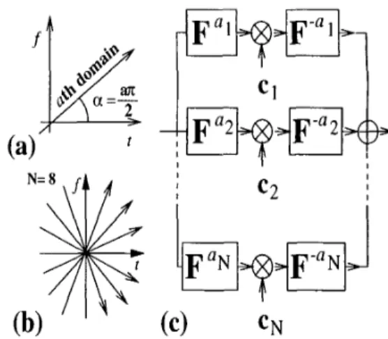
1. For instance, we may take the a k uniformly spaced in this interval.

The corresponding fractional Fourier domains are illus- trated in figure l b . We define the FFDD of H as

N

H N , x N , =

F i e k

[ A k ] N , x N , ( F & : k ) t , ( 7 ) k = l

where A , , A2,

. .

.

,

A N are diagonal matrices each of whose N’ = min(N,, N,) elements c k j , j = 1 , 2 , .

.

,

N‘

are in general complex numbers. It will sometimes be

a convenient way t o represent these diagonal elements

a

=-i-

t

Figure 1: (a) The a t h fractional Fourier domain. T h e

a = 0th and a = 1st domains are the ordinary time

( t )

and frequency

(f)

domains. (b) N equally spaced fractional Fourier domains. (c) Block diagram of the FFDD.

c k l , c k 2 ,

. . .

,

C k N ’ for any k in the form of a column vec-

tor Ck. When H is Hermitian (skew-Hermitian), C k is

real (imaginary). We also note that

( F G : k ) t

= F$c.

The FFDD always exists and is unique, as will be dis- cussed further below.

Comparing and contrasting the FFDD with the SVD will help gain insight into the FFDD. If we compare one term on the right-hand side of (7) with the right- hand side of (2), we see that they are similar in t h a t they both consist of 3 terms of corresponding dimen- sionality, the first and third being unitary matrices and the second being a diagonal matrix. But whereas the columns of U and V constitute orthonormal bases specific t o H, the columns of FGBk and

FG:k

constitute orthonormal bases for the akth fractional Fourier domain. Customization of the decomposition is achieved through the coefficients c k j (and perhaps also the or-

ders a k ) .

Denoting the j t h columns of F i : k and FG:k as

[ F N B k ] j and [ F & : k ] j respectively, it now becomes possi-

ble t o write the kth term of the summation in (7) as a n outer product of the form

cj=l

c k j [ F i : k ] j ( [ F L : k ] j ) t

so that (7) can be rewritten as

N‘

N N ‘

H

7;

c k j [ F & r k ] j ( [ F i : k ] j ) t - (8) k = l j=1

To a certain extent, the inner summation resembles the outer-product form of the SVD given in (3). The

N , x N , matrices [ F L : k ] j ( [ F i : k ] j ) t are of unit rank

since they are the outer product of vectors. We will

(3)

denote these matrices by P k j so that

This equation is simply an expansion of H in terms of the basis matrices p k j , 1

5 k

5 N ,

1

5

j

5 N’,

where the c k j serve as the weighting coefficients of the

expansion.

When H is a square matrix of dimension N, the FFDD takes the simpler form

N

H = F-”k A k

(F-”’)’,

(10) k = l

where all matrices are

N

x

N.

Equation (9) is a linear relation between the matrices H and c k 3 with the four-dimensional tensor P k j

representing the transforniation between them. Let

3-1

denote a column ordering of the matrix

H,

with dimensions N c N , x 1. Also let C denote the

NN’

x 1

column vector obtained by stacking the column vectors

c 1

,

c 2 , . .

. ,

C N on top of each other. Notice that we al-

ways have

NN’

= max(N,,N,)min(N,,N,) = N T N c . These column orderings determine a corresponding ordering which converts the four-dimensional tensor (or two-dimensional array of matrices) P k g into a square matrix P of dimensions N c N , x

N,N,.

(The vector obtained as the column ordering of the matrix P k j for

a specific k j , goes into the [ ( k - 1)N’

+

j ] t h column of the matrix

P.)

Now, we can write (9) as the linear square matrix equation

3-1

=

PC.

This equation will have a unique solution for C and thus Ck3 if and only if the columns of

P

are linearly independent. Since the columns of

P

are merely column orderings of the basis matrices Pk, , this is the same as linear independence of these basis matrices. Recalling the definition of these matrices (just before (9) ), their linear independence follows from the fact that the inner, product of any column of Fa with any column of Fa (a’

#

a ) is always nonzero. Thus the F F D D always exzsts and as unzque

(for given ak).

4. APPLICATIONS

Let H denote a linear matrix operator. Equation (7)

represents a decomposition of this operator into

N

terms. Each term, taken by itself, corresponds t o filtering in the akth fractional Fourier domain [6, 21, where an nkth order forward transform is followed by multiplication with a filter function c k and concluded with an

inverse nkth order t,ransform. If a k = 1, this corre-

sponds to ordinary Fourier domain filtering. If a k = 0,

this corresponds t o multiplication of a signal with a

filter function directly in the time domain. All terms taken together, the FFDD can be represented by the block diagram shown in figure IC and interpreted as

the decomposition of an operator into fractional Fourier domain filters of different orders. An arbitrary linear system H will in general not correspond to multiplica- tive filtering in the time or frequency domain or in any other single fractional Fourier domain. However,

H

can always be expressed as

a

combination of filtering operations in different fractional domains.

A

s u f i c i e n t

number of different-ordered fractional Fourier d o m a i n

filtering operations “span” the space of all linear oper-

ations. The fundamental importance of the FFDD is

that it shows how an arbitrary linear system can be decomposed into this complete set of domains in the time-frequency plane.

If

H represents a time-invariant system, all filter CO- efficients except those corresponding to a k = 1 will be

zero. More generally, different domains will make varying contributions to the decomposition. By eliminating domains for which the coefficients C k l

,

C k 2 ,

.

. ,

C k N ‘ are small, significant savings in storing and implementing

H becomes possible. This procedure, which we refer t o

as pruning the FFDD, is the counterpart of truncating

the SVD. An alternative to this selective elimination procedure will be referred to as sparsening, in which we simply work with a more coarsely spaced set of domains.

In any event, the resulting smaller number of domains will be denoted by

M

<

N.

The upper limit of the summation in (7) is replaced by

M

and the equality is replaced by approximate equality, leading us to

3-1

M

PC.

If we solve this in the least-squares

sense, minimizing

113-1

-

PC(1,

we can find the coefficients resulting in the best M - d o m a i n approximation

to H. This procedure amounts t o projecting

H

onto the subspace spanned by the A4 basis matrices, which now do not span the whole space.

Since the fractional Fourier transform can be com- puted in O ( N log N) time, implementation of the pruned version of figure IC takes O ( M N log N) time.

If

an acceptable approximation to

H

can be found with a rela- tively small value of M , this can be much smaller than the time O(N,Nc) associated with direct implementation of the linear system. Likewise, optical implementation requires a space-bandwidth product of

O( M N ) ,

as opposed to O(N,N,) for direct implementation [7]. In passing, we note that the pruned FFDD is directly related to the concept of parallel filtering [8, 91.

As an example, we consider the problem of recov- ering a signal consisting of multiple chirp-like compo- nents, which is buried in white Gaussian noise such that

(4)

the signal-to-noise ratio is 0.1. We assume the signal consists of 6 chirps with uniformly distributed random amplitudes and time shifts, and that the chirp rates are known with a f 5 % accuracy. We find that the general linear optimal Wiener filter H for this problem can be approximated with a mean-square error of 5.2% by using only M = 6 domains. H can also be approximated by truncating (3) to

M

terms, leading to an implementation time of

O ( M N ) .

For the present example,

M = 6 results in an error of 20%, demonstrating an instance where the FFDD yields better accuracy than the SVD.

Next we consider restoration of images blurred by a space-varying point-spread function whose diameter increases linearly with position. This time we use the

demic Press, San Diego, California, 1999, pp. 239- 291.

[2]

H.

M. Ozaktas, B. Barshan, D. Mendlovic, and L. Onural, “Convolution, filtering, and multiplexing in fractional Fourier domains and their relation to chirp and wavelet transforms”, J. Opt. Soc. Am.

A vol. 11, 1994, pp. 547-559.

[3] L. B. Almeida, “The fractional Fourier transform and time-frequency representations”, IEEE Trans.

Sig. Proc. vol. 42, 1994, pp. 3084-3092.

[4] C. Candan, M. A. Kutay, H.

M.

Ozaktas “The Discrete Fractional Fourier Transform” to appear

in IEEE Trans. Sag. Proc., 2000.

M-domain expansion as a constraint on the linear re- covery filter and optimize directly over the coefficients

C k j to minimize the mean-square estimation error. The

error is found t o be 7% for

M

= 5. One may con-

[5]

S.

C. Pei and M. H. Yeh, “Improved discrete fractional Fourier transform”, Opt. Lett., vol. 22, no. 14, 1995, pp. 1047-1049.

struct a similar constrained optimization problem by using the truncated SVD. However, this leads to a much more difficult nonlinear optimization problem because

uj and vj in (3) are also unknowns, whereas the only

unknowns in (7) are the

&,

leading t o a linear optimization problem.

Other potential applications other than fast implementation of linear systems include data compression, statistically-optimum filtering, and regularization of ill- posed inverse problems, all of which may be based on the same basic idea of appropriately pruning or weighting the different domains.

We have not addressed the problem of optimally choosing the orders a k , which corresponds to choosing

the basis matrices. When M = N , the basis matrices form a complete set and any choice is acceptable. How- ever, certain choices may offer better numerical stabil- ity. When M

<

N I the choice of a k may reflect our

knowledge about the ensemble of matrices H we wish

[6] M. A. Kutay, H. M. Ozaktas,

0.

Arikan, and

L.

Onural, “Optimal filtering in fractional Fourier domains”, IEEE Trans. Sig. Proc. vol. 45, 1997, pp. 1129-1 143.

[7] H. M. Ozaktas and D. Mendlovic, “Fractional Fourier optics”, J . Opt. Soc. Am. A vol. 12, 1995, pp. 743-751.

[8] M. A. Kutay, M. F. Erden, H. RI. Ozaktas,

0.

Arikan, C. Candan, and

0.

Guleryuz, ‘‘Cost- Efficient Approximation of Linear Systems with Repeated and Multi-channel Filtering Configura- tions,” Proc. IEEE Int. Conf. Acous., Speech and

Sag. Proc., Seattle, May 12-15 1998.

[9] M. A. Kutay,

M.

F. Erden,

H.

M. Ozaktas,

0.

Arikan,

0.

Guleryuz, and C. Candan, “Space- Bandwidth Efficient Realizations of Linear Sys-

terns”, to appear in Opt. Lett..

to approximate. This knowledge may be statistical or in the form of restrictions on the set of matrices possible. It is also possible to choose the orders optimally for a single specific matrix.

[lo] B. Barshan, M. A. Kutay, and H.

M.

Ozaktas, “Optimal Filtering with Linear Canonical Trans- forms”, Opt. Commvn., vol. 135, 1997, pp. 32-36.

A

natural extension of the FFDD would be the lin-

ear canonical domain decomposition (LCDD) based on linear canonical transforms [IO].

5. REFERENCES

[l] H. M. Ozaktas,

M.

A. Kutay and D. Mendlovic, “Introduction to the fractional Fourier transform and its applications”, in: P. W. Hawkes, ed., Ad-

vances in Imaging and Electron Physics 106, Aca-