IDENTIFICATION OF BUTTERFLY SPECIES
USING MACHINE LEARNING AND IMAGE
PROCESSING TECHNIQUES
2020
DOCTOR OF PHILOSOPHY
COMPUTER ENGINEERING
Ayad Saad ALMRYAD
IDENTIFICATION OF BUTTERFLY SPECIES USING MACHINE LEARNING AND IMAGE PROCESSING TECHNIQUES
Ayad Saad ALMRYAD
T.C.
Karabuk University Institute of Graduate Programs Department of Computer Engineering
Doctor of Philosophy
Assist. Prof. Dr. Hakan KUTUCU
KARABUK February 2020
“I declare that all the information within this thesis has been gathered and presented in accordance with academic regulations and ethical principles and I have according to the requirements of these regulations and principles cited all those which do not originate in this work as well.”
ABSTRACT
Ph. D. Thesis
IDENTIFICATION OF BUTTERFLY SPECIES USING MACHINE LEARNING AND IMAGE PROCESSING TECHNIQUES
Ayad Saad ALMRYAD
Karabük University Institute of Graduate Programs Department of Computer Engineering
Thesis Advisor:
Assist. Prof. Dr. Hakan KUTUCU February 2020, 70 pages
In today‟s competitive conditions, producing fast, inexpensive and reliable solutions are objectives for engineers. Development of artificial intelligence and the introduction of this technology to almost all areas have created a need to minimize the human factor by using artificial intelligence in the field of image processing, as well as to make a profit in terms of time and labor. In this thesis, we propose an automated butterfly species identification model using artificial neural and deep neural networks.
The study in the thesis consists of two stages. In the first stage, we studied on lab-based butterfly images taken on under a fixed protocol. The species of butterflies in these images are identified by expert entomologists. We used a total of 140 images for lab-based butterfly images of 10 species. After applying some preprocess to the images such as histogram equalization and background removing, we extracted
several features from the butterfly images. Finally, we used an artificial neural network in MATLAB version R2014b using the Neural Network Toolbox for butterfly identification. The ANN model achieved an accuracy of 98%.
In the second stage of the thesis, we studied on field-based butterfly images. We collected 44659 images of 104 different butterfly species taken with different positions of butterflies, the shooting angle, butterfly distance, occlusion, and background complexity in the field in Turkey. Since many species have a few image samples we constructed a field-based dataset of 17769 butterflies with 10 species. Convolutional Neural Networks (CNNs) implemented by Python were used for the identification of butterfly species. Comparison and evaluation of the experimental results obtained using three different network structures are conducted. Experimental results on 10 common butterfly species showed that our method successfully identified various butterfly species.
Key Words : Artificial intelligence, deep learning, computer vision, butterfly species recognition, feature extraction, feature selection.
ÖZET
Yüksek Lisans Tezi
MAKĠNE ÖĞRENMESĠ VE GÖRÜNTÜ ĠġLEME TEKNĠKLERĠ KULLANILARAK KELEBEKLERĠN TANIMLANMASI
Ayad Saad ALMRYAD
Karabük Üniversitesi Lisansüstü Eğitim Enstitüsü Bilgisayar Mühendisliği Anabilim Dalı
Tez DanıĢmanı:
Dr. Öğr. Üyesi Hakan KUTUCU ġubat 2020, 70 sayfa
Günümüzün rekabetçi koşullarında, hızlı, ucuz ve güvenilir çözümler üretmek mühendisler için bir hedeftir. Yapay zekanın geliştirilmesi ve bu teknolojinin neredeyse tüm alanlara tanıtılması, görüntü işleme alanında yapay zekayı kullanarak insan faktörünü en aza indirmenin yanı sıra zaman ve emek açısından kar elde etme ihtiyacını yarattı. Bu tezde, yapay sinir ve derin sinir ağlarını kullanarak otomatik bir kelebek türü tanımlama modeli öneriyoruz.
Tezdeki çalışma iki aşamadan oluşmaktadır. Ġlk aşamada, sabit bir protokol altında alınan laboratuvar tabanlı kelebek görüntüleri üzerinde çalıştık. Bu görüntülerdeki kelebek türleri uzman entomologlar tarafından tanımlanmıştır. 10 türün laboratuvar tabanlı kelebek görüntüleri için toplam 140 görüntü kullandık. Histogram eşitleme ve arka plan kaldırma gibi görüntülere bazı ön işlemler uyguladıktan sonra, kelebek görüntülerden çeşitli özellikler çıkardık. Son olarak, kelebek tanımlama için Neural
Network paketi kullanılarak MATLAB R2014b versiyonunda yapay sinir ağı kullandık. YSA modeli % 98'lik bir doğruluk elde etmiştir.
Tezin ikinci aşamasında alan bazlı (doğadan) kelebek görüntüleri üzerinde çalıştık. Türkiye'de doğada çekilmiş farklı pozisyon, çekim açısı, kelebek mesafesi ve arka plan karmaşıklığı ile alınan 104 farklı kelebek türünden 44659 görüntü topladık. Birçok türün birkaç görüntü örneği olduğundan, 10 tür içeren 17769 kelebeğin alan tabanlı bir veri kümesini oluşturduk. Kelebek türlerinin tanımlanmasında Python tarafından uygulanan Evrişimli Sinir Ağları (CNN) kullanılmıştır. Üç farklı ağ yapısı kullanılarak elde edilen deneysel sonuçların karşılaştırılması ve değerlendirilmesi yapılmıştır. 10 yaygın kelebek türü üzerinde yapılan deneysel sonuçlar, yöntemimizin çeşitli kelebek türlerini başarıyla tanımladığını göstermiştir.
Anahtar Kelimeler : Yapay zeka, derin öğrenme, bilgisayarla görme, kelebek türlerinin tanınması, özellik çıkarma, özellik seçimi.
ACKNOWLEDGMENT
First of all, I would like to express my gratitude to Allah, who has given me these days, always protects me, gives me strength and makes me successful.
I would like to thank Dr. Hakan KUTUCU whom I have benefited from his extensive knowledge and experience in the planning, research, execution, and formation of this thesis. In addition, I would like to thank all of my teachers and colleagues who have always supported me with their help, knowledge, and experience during my undergraduate and graduate education.
Finally, I thank my dear family for their patience, self-sacrifice, and support, and for all physical and spiritual assistance with my whole heart.
CONTENTS Page APPROVAL ... ii ABSTRACT ... iv ÖZET... vi ACKNOWLEDGMENT ... viii CONTENTS ... ix
LIST OF FIGURES ... xii
LIST OF TABLES ... xiv
SYMBOLS AND ABBREVIATIONS INDEX... xv
PART 1 ... 1
INTRODUCTION ... 1
PART 2 ... 3
THEORETICAL BACKGROUND ... 3
PART 3 ... 9
MATERIALS AND METHODS ... 9
3.1. MATERIALS ... 9
3.2. METHOD ... 9
PART 4 ... 20
ARTIFICIAL NEURAL NETWORK ... 20
4.1. ANN CHARACTERISTICS ... 22
4.2. NETWORK STRUCTURE ... 22
4.3. IMAGE DATA PRE-PROCESSING FOR NEURAL NETWORKS ... 23
PART 5 ... 24
Page
PART 6 ... 28
METHODOLOGY ... 28
6.1. ADVANTAGES AND DISADVANTAGES ... 29
6.2. FOREGROUND / BACKGROUND DETECTION ... 30
6.3. MATERIALS ... 31
6.3.1. Dataset ... 31
6.3.1.1. Field-Based Images ... 31
6.3.1.2. Lab-Based Images ... 32
6.3.2. Image Preprocessing Step ... 33
6.3.3. Implementation ... 34
6.3.4. Explanation of The Script ... 35
6.4. EXPERIMENTAL TESTS... 38
6.4.1. Field-Based Images ... 38
6.4.2. Lab-Based Images ... 40
PART 7 ... 43
LOCAL BINARY PATTERN ... 43
7.1. THE BASIC LBP ... 43 7.2 UNIFORM LBP ... 44 7.3. CENTER SYMMETRIC LBP ... 45 PART 8 ... 47 FEATURE EXTRACTION ... 47 PART 9 ... 55
DEEP NEURAL NETWORKS ... 55
9.1. TRANSFER LEARNING ... 58
9.2. VGG16 - VGG19 ... 59
9.3. RESNET 50 ... 60
Page
PART 10 ... 63
CONCLUSION ... 63
REFERENCES ... 65
LIST OF FIGURES
Page
Figure 3.1. Flowchart - explains the steps that will be used in this study. ... 9
Figure 3.2. Block diagram of the experimental design. ... 10
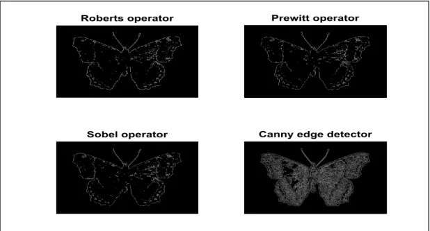
Figure 3.3. Edge detection using various operators. ... 11
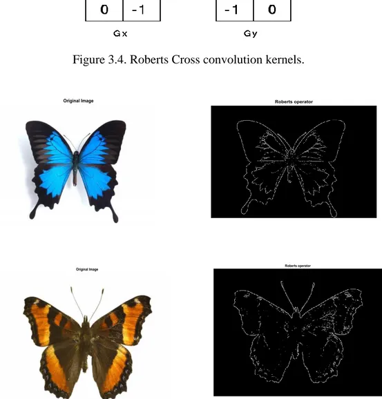
Figure 3.4. Roberts Cross convolution kernels. ... 12
Figure 3.5. Robert‟s operator of the butterfly image... 12
Figure 3.6. Masks for Sobel edge detection operator. ... 13
Figure 3.7. Sobel edge detector of butterfly image. ... 13
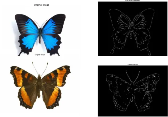
Figure 3.8. Masks for Prewitt edge detection operator. ... 14
Figure 3.9. Prewitt Operator of the butterfly image. ... 14
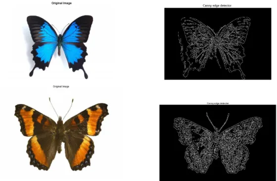
Figure 3.10. Canny edge detector of the butterfly image. ... 15
Figure 3.11. Special effects in an image using different types of noise... 16
Figure 3.12. Salt and pepper noise of butterfly image. ... 16
Figure 3.13. Gaussian noise of butterfly image. ... 17
Figure 3.14. Speckle noise of butterfly image. ... 18
Figure 3.15. Histogram modeling. ... 18
Figure 4.1. A general overview of ANN. ... 20
Figure 4.2. Artificial neural network characteristics. ... 22
Figure 6.1. Flowchart to explain the research methodology. ... 29
Figure 6.2. Sample images in the field-based dataset. ... 32
Figure 6.3. Lab based butterfly images with 14 butterfly species... 33
Figure 6.4. Image preprocessing steps. ... 34
Figure 6.5. Python script of the preprocessing step. ... 35
Figure 6.6. Successful segmentations. ... 39
Figure 6.7. Unsuccessful segmentations. ... 40
Figure 6.8. All steps of the segmentation. ... 41
Figure 6.9. Successful segmentation of lab-based images. ... 41
Figure 7.1. The steps for obtaining the final feature histogram representation using LBP. ... 43
Figure 7.2. Basic LBP computation for a 3 × 3 image patch and the corresponding LBP code. ... 44
Page
Figure 7.3. Circularly symmetric neighbor sets. ... 45
Figure 7.4. Computing the CSLBP pattern for an 8 neighborhood of pixels. ... 46
Figure 8.1. After segmentation. ... 47
Figure 8.2. ULBP and HSV components of a given butterfly. ... 49
Figure 8.3. Schematic diagram of an ANN for prediction of butterfly species with one input layer, one hidden layer, and one output layer. ... 53
Figure 8.4. The view of the ANN in Matlab. ... 53
Figure 8.5. The performance values of the ANN model with one hidden layer and 10 neurons. ... 54
Figure 9.1. CNN architecture. ... 55
Figure 9.2. Convolution process. ... 56
Figure 9.3. Max and average pooling. ... 57
Figure 9.4. Softmax function... 57
Figure 9.5. A visualization of the VGG architecture. ... 59
Figure 9.6. ConvNet configurations for VGGNET. ... 60
Figure 9.7. Resnet architecture. ... 61
Figure 9.8. VGG-16 Accuracy and loss curve. ... 62
Figure 9.9. VGG-19 Accuracy and loss curve. ... 62
Figure 9.10. ResNet50 Accuracy and loss curve. ... 62
LIST OF TABLES
Page Table 6.1. Name and the number of images per butterfly‟s genus in the dataset. ... 32 Table 8.1. Features of 140 butterflies... 49 Table 9.1. The real-world butterfly species images labeled by users. ... 61
SYMBOLS AND ABBREVIATIONS INDEX
SYMBOLS
: Spatial Gradient
: Speckle noise distribution image : the input image
: the uniform noise image : the threshold value : the circle of radius
: the average of texture features : the deviation of texture features : the energy of texture features : the entropy of texture features : the correlation of texture features : the matrix of size
: the maximum value for the ULBP matrix Μ: : the mean
: the standard deviation. : the padding size : the stride number : fully-connected layers : input layer
: convolution layer : pooling layer : output layer
ABBREVIATIONS
RESNET50 : Deep Residual Learning for Image Recognition VGG-16 – 19 : Visual Geometry Group - 16
CNN : Convolutional Neural Networks
RGB : Red-Green-Blu
HSV : Hue-Saturation-Value
ULBP : Uniform Local Binary Patterns LBP : Local Binary Patterns
CSLBP : Center Symmetric Local Binary Patterns SIFT : Scale-Invariant Feature Transform ANN : Artificial Neural Network
MSE : Mean Squared Error
ICA : Linear Discriminant Analysis PCA : Principal Component Analysis SVM : Support vector Machines
ED : Edge Detection
GM : Graph Modeling
JPEG : Joint Photographic Experts Group TIFF : Tag Image File Format
PART 1
INTRODUCTION
Butterflies are insects in the order Lepidoptera. The number of butterfly species in the world varies from 15000 to 21000 according to a recent estimate in [1]. Due to various species, high similarity and the characteristics of the distinction of butterflies are not evident, the identification and classification of butterflies have the problems of low accuracy and slow recognition. Furthermore, the number of taxonomists and trained technicians have decreased dramatically.
The discrimination between butterfly species requires expertise and time, which is not always available, but after the development of software that identifies butterfly species by extracting features from images, the need for experts will reduce. There are two main problems in the existing butterfly species identification research based on computer vision techniques. First, collecting the butterfly dataset is difficult, identifying is time-consuming work for entomologists, and the number of butterflies included in the butterfly dataset is not comprehensive. Second, the butterfly pictures used for training are all pattern pictures with obvious morphological features, lacking the ecological pictures of butterflies in nature. Furthermore, the differences between the two pictures are obvious that makes the combination of research and production difficult and the recognition accuracy is low [2]. Therefore, it is of great importance to make research on the automatic identification of butterflies and improve its accuracy and efficiency. The development of tools for automating the identification of butterfly species has an important contribution to the literature.
This thesis is organized as follows: In Part 2, we discuss the theoretical background of insect classification and identification. We introduce image processing techniques related to butterfly segmentation in Part 3. We give a short review of artificial neural network (ANN) and the ANN architecture to identify butterfly species in Part 4. We
give an extensive literature review of insect classification researches in Part 5. The field butterfly image dataset and the methodology are discussed in Part 6. We introduce local binary patterns which will be used to extract some features from the butterflies in Part 7. In Part 8, we give the features which are extracted and used as input for the artificial neural network. A technical approach based on the different convolutional neural network architectures is introduced in Part 9. Finally, the conclusion section concludes the thesis.
PART 2
THEORETICAL BACKGROUND
Due to various species, high similitude and the attribute of the divergence is not evident, the identification and classification of butterflies have the complications of low precision and steady identification. Therefore, it is very significant to do research on the automatic recognition of butterflies and better its accuracy and orderliness. The development of tools for automating the identification of butterfly species has an important contribution to the literature. The discrimination between butterfly species requires expertise and time, which is not always available, but after the development of software that identifies some butterfly species by extracting features from butterflies.
There exist two main problems in the be living butterfly species recognition research. Firstly, collecting the butterfly set of information is hard, identifying is time-consuming work for entomologists, and various butterflies comprised in the butterfly set of information is not thorough. Secondly, the pictures of the butterflies geared towards training are all pattern pictures having obvious morphological features, missing the ecological pictures of butterflies in the natural ecological environment. Furthermore, the unlikenesses between two pictures are apparent making the merge of production and experimentation difficult and the identification correctness is low.
Kaya et al. [3] proposed two novel local binary patterns (LPB) descriptors for detecting special textures in images. One is established on the correlation between the sequential neighbors of a center pixel with a defined distance and the other is established on determining the neighbors in the same orientation through the central pixel parameter. They tested their descriptors to identify butterfly species on lab-based images of 140 butterflies collected in Van city of Turkey. The highest accuracy they obtained for classifying butterflies by the artificial neural network is
95.71%. Kaya and Kaycı [4] developed a model for butterfly identification depending on color and texture characteristics by the artificial neural network using the gray level co-occurrence matrix with different angles and distances. The correctness of their method reached 92.85%. Wen and Guyer [5] developed a model which combines local and global features for insect classification via five classifiers that are normal densities based linear classifier (NDLC), the minimum least-square linear classifier (MLSLC), nearest mean classifier (NMC), K-nearest neighbor classifier (KNNC) and decision tree (DT). Their experimental results tested on images obtained from actual field trapping for training yielded the classification rate of 86.6%.
Xie et al. [6] proposed a learning model for the classification of insect images by the use of advanced multiple-task sparse representation and multiple-kernel learning techniques. They tested the proposed model on 24 common pest species of field crops and compared it with some recent methods.
Feng et al. [7] improved an insect species identification and retrieval system established on wing characteristics of moth images. Their retrieval system is based on CBIR architecture not being about having a final answer but just issuing a match-list to the user.
Yao et al. [8] designed a model to automate rice pest identification using 156 features of pests. The authors tested the proposed model on a few species of Lepidoptera rice pests with middle size using the support vector machine classifier.
Another study for pest recognition was done by Faithpraise et al. using the k-means clustering algorithm and correspondence filters [9]. Leow et al. [10] developed an automated identification system of copepod specimens by extracting morphological features and using ANN. They used seven copepod features of 240 sample images and estimated an overall accuracy of 93.13%.
Zhu and Zhang [11] proposed a technique to classify lepidopteran insect images by integrated region matching and dual-tree complex wavelet transform. They tested the
method on a database including 100 lepidopteran insects of 18 families and estimated the identification correctness of 84.47%.
Mayo and Watson [12] showed how effective data mining techniques could be for the recognition of species. They used WEKA which is a data mining tool with different classifiers such as Naïve Bayes, instance-based learning, random forests, decision trees, and support vector machines. WEKA was able to achieve an accuracy of 85% using support vector machines to classify live moths by species.
Another work for identification of live moths was conducted by Watson et al [13] who proposed an automated identification tool named DAISY. Silva et al. [14] aimed to investigate the best combination of feature selection techniques and classifiers to identify honeybee subspecies. They found the best pair as the combination of Naïve Bayes classifier and the Correlation-Based feature selector in their experimental results among seven combinations of feature selectors and classifiers.
Wang et al. [15] designed an identification system of insect images at the order level. They extracted seven features from insect images. However, the authors manually removed some attached to insects such as pins. Their method has been tested on 225 specimen images from nine orders and sub-orders using an artificial neural network with an accuracy of 93%.
The discrimination between butterfly species requires expertise and time, which is not always available, but after the development of software that identifies some butterfly species by extracting features from butterflies' wings, the species identification became faster and efficient.
The development of the system to identify insect species needs great efforts. Machine learning techniques like Deep Learning, Convolutional Neural Networks (CNNs), principal component analysis (PCA), linear discriminant analysis (LDA), artificial neural networks (ANNs), support vector machines (SVMs) can be used to create automated identification system.
Pattern recognition and machine learning are jointly studied two branches of artificial intelligence. Pattern recognition use experience gained from improvements in machine learning and image processing techniques. Many studies on pattern recognition include image processing and machine learning. In these systems, image processing techniques are used to identifying the objects in input images and then machine learning is used to learn the system for the change in pattern. With the advent of new methods and techniques on related fields, pattern recognition can be used more and more computer-aided diagnosis, recognition and categorization of objects, etc.
In order to study with images on computers, some steps are required to digitalize the input images. A digital image may be defined as mathematically a two-dimensional function f(x, y), where „x‟ and „y‟ represent the spatial coordinates of digital images and the amplitude of „f‟ at any pair of coordinates is called the intensity of the image at that point. If the image can be stored in computer memory with finite discrete quantities then it is called a digital image.
In order to get some useful information or conversion from analog space to digital space on images, Image processing techniques which include specific operations are required. These techniques rely on carefully designed algorithms. Performed automatically, are changes that take place in images through these algorithms of image processing. The problem of extracting information from images and interpreting this information has been the incentive for the research community of image processing. Image processing techniques can be used in many fields, including medicine, business, industry, military.
Image processing is improved by interdisciplinary fields with contributions from different arms of science like mathematics and physics, computer and electrical engineering and optics. For the application area, image processing is closely related to the other artificial intelligence fields such as machine learning, human-computer interaction, pattern recognition. The different steps associated with image processing comprise importing the image from an optical scanner or digital camera, analyzing and modifying the image (data compression, image enhancement, and filtering), and
creating the desired output image. The general purpose of image processing as a system is the conversion of digital space into a standard pose and obtaining identifiable entity on a uniform background.
Image enhancement can be performed manually or automatically. Manually, the user carried out using Image or special computer software (Photoshop, gimp) may produce finer image pre-processing results. It‟s preferable to use entirely automated methods to build systems with a large number of images as it is time-consuming to use the manual image processing methods.
In general, the first step in image processing is image acquisition. Image processing accuracy highly depends on this step. A sophisticated camera or modern phone camera can be used to obtain high quality and sharp images. In this step some images distributed from the internet web for training and testing image processing systems. It is also of importance when gathering images to reduce glare and shadows. It is recommended to include in the image some known size reference or scale. Wing images can also be shot by scanning the wings. Without leading to occlusion of the areas of interest, the wings should be well mounted in the images tenanting the largest area possible. Images can be of grayscale or color stored in formats like JPEG, TIFF, or others.
After the image acquisition step, digital image processing is performed. This process consists of two sequential sub-processes: image pre-processing and feature extraction. The First sub-process tries to improve input images and the modified image is its output. This step tries to solve many problems such as noise reduction, occlusion removal, etc. Taking an image as input this step produces a reformed image as an output, which should be suitable for the feature extraction step.
The latter sub-process focuses to extract useful sets of computations either characterizing the whole image or a few components thereof and the output comprises information about the content of the image. The image preprocessing sub-process may perform noise removal, enhancement, and segmentation. In many previous studies, Matlab has been used to facilitate the process of image processing
and testing for accurate results before they are implemented in the system or programming language such as Java, C#, Python, etc. In this section, first, we need to process images using Matlab, and we will implement three stages of image processing (Edge Detection (ED), Noise, Graph Modeling (GM)) for a pure and accurate image to be used for matching later.
PART 3
MATERIALS AND METHODS
3.1. MATERIALS
In principle, some of the images were downloaded from the internet to use for the system experience. Each image of an aerial view with a natural background. Since the two sides of the butterfly wing are different, so we will choose the boundary of the butterfly wing to investigate to maintain the consistency. As well to make the image extraction process clear and high resolution, it is best to remove the background.
3.2. METHOD
In this thesis, we will study on feature extraction techniques and CNN architectures in the context of the winged insect (butterflies) classification. The general flowchart is given in Figure 3.1.
The idea of using (Edge Detection (ED), Noise, Graph Modeling (GM)) for butterfly species illustration is inspired by the reality that butterflies can be seen as a composition of micro-patterns which are consequently expressed by this operator. The method for classifying the images suggested in this study is based on texture descriptors obtained from the butterfly images. As demonstrated in Figure 3.2, into four major steps, is how divided our approach can be:
Figure 3.2. Block diagram of the experimental design.
The objective of image preprocessing is cleaning images from various noises. In image processing, noise may occur in the transforming phase of the image from analog to digital form or during the image transmission phase.
In order to perform a useful pre-processing process the key step is to determine the region of objects in the input image. This step is called edge detection. In literature, there are well-known methods for edge detection (Robert‟s operator, Prewitt operator, Sobel operator, and Canny edge detector). If the image contains only one object, these operators help to identify to points which are must be a focus. Figure 3.3 shows output images with different edge detection algorithms on a sample butterfly image.
The general approach of edge detection has four steps listed as follows:
1. Smoothing: In this step, noise is detached without spoiling the true edges. 2. Enhancement: To uncover the true edges, filters are applied to the image.
This step may be called sharpening.
3. Detection: determine which edge pixels should be gotten rid of as noise and which should be kept (usually, thresholding provides the criterion used for detection).
4. Localization: determine the exact location of an edge (sub-pixel resolution might be required for some applications, that is, estimate the location of an edge to better than the spacing between pixels). Edge thinning and linking are usually required in this step.
Some software (MATLAB) or libraries (OpenCV) has released to using to edge detection. These libraries include many special methods for edge detection (Robert‟s, Prewitt, Sobel, Canny operators, etc.).
Figure 3.3. Edge detection using various operators.
Robert‟s operator: The Roberts Cross operator performs on an image a simple, rapid to compute, 2-D spatial gradient measurement. It thus highlights regions of high
spatial frequency which often correspond to edges. In its most common usage, the input to the operator is a grayscale image, as is the output. Pixel values at each point in the output represent the estimated absolute magnitude of the spatial gradient of the input image at that point. Horizontal derivative approximate as Equation 3.1 and vertical derivative approximate as Equation 3.2. It‟s convolution kernel matrices are given in Figure 3.4. The output effect of the Robert Cross operator is shown in Figure 3.5.
(3.1
(3.2)
Figure 3.4. Roberts Cross convolution kernels.
Sobel edge detector: When applied to gray-scale images, the Sobel operator calculates the gradient of each pixel‟s brightness intensity, giving the direction of the larger possible increase from black to white, and also calculates the sum of that direction‟s shift. A 2-D spatial gradient analysis is performed on an image by the Sobel operator. It is usually used in an input grayscale picture to find the estimated absolute gradient magnitude at each point. The Sobel edge detector uses a pair of 3x3 convolution masks, one estimating the x-direction gradient (columns) and the other estimating the y-direction (rows) gradient. It‟s very similar to the director in Prewitt. It is also a derivative mask used for the detection of edges. It also measures the horizontal and vertical edge detection. It‟s got better control of noise. The operator consists of the following pair of kernels of 3x3 convolution (Figure 3.6). The output effect of a Sobel operator is shown in Figure 3.7.
Figure 3.6. Masks for Sobel edge detection operator.
Prewitt edge detector: It is used for edge detection than detect two types of edge horizontal or vertical. The edges are computed by using the difference between corresponding pixel intensities of an image. The masks used for edge detection are all known derivative masks and this operator is called the derivative operator. The kernel matrices are given in Figure 3.8. Also, the output image of this operator is given in Figure 3.9.
Figure 3.8. Masks for Prewitt edge detection operator.
Figure 3.9. Prewitt Operator of the butterfly image.
Canny Edge Detector: The system of Canny seeks edges by looking for local gradient maxima. The gradient will be determined using a Gaussian filter derivative. The method uses two thresholds to detect strong and weak edges and includes weak
edges only when related to strong edges in the performance. Therefore, this approach can rarely be fooled by noise and more liked than the others. The output image of this operator is given in Figure 3.10.
Figure 3.10. Canny edge detector of the butterfly image.
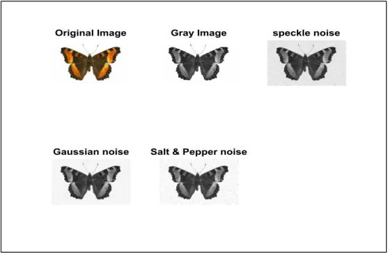
There are various types of noise (speckle, Gaussian, salt-and-pepper). Such forms of noise can be used as special effects in the picture using a butterfly image as shown in Figure 3.11. In this step, RGB-to-gray is first converted and different types of noise are applied to the image through the software.
Figure 3.11. Special effects in an image using different types of noise.
Salt and pepper noise: Due to sharp and sudden changes in the image signal, this noise comes about in the image as shown in Figure 3.12. For images that are distorted by salt and pepper noise, the maximum and minimum values in the dynamic range are taken by the noisy pixels. In general, salt and pepper noise is caused by malfunction of pixel elements in-camera sensors, faulty memory locations or timing errors in the digitization process.
Figure 3.12. Salt and pepper noise of butterfly image.
Gaussian noise: is evenly distributed over the signal. This infers that the sum of the true pixel value and a random Gaussian distributed noise value are each pixel in the noisy image. At every level, the noise is independent of the pixel value size. White
Gaussian noise is a unique case, with the distribution of values in a similar way and at any pair of time-independent statistically. White noise inherits its name from white light. During the processing, for example, sensor noise brought about by poor lighting or high temperature or transmission, the main sources of Gaussian noise in digital images emerge. Figure 3.13 is shown an example of Gaussian noise production on the butterfly image.
Figure 3.13. Gaussian noise of butterfly image.
Speckle noise: in contrast to the Gaussian and salt pepper noise, speckle noise is multiplicative kind of noise. By multiplying a random value with picture pixel values this noise can be cast and represented as
(3.3)
P standing for speckle noise distribution image, I stand for the input image and n for the uniform noise image by means o and variance v. The output image of the speckle noised butterfly image is given below in Figure 3.14.
Figure 3.14. Speckle noise of butterfly image.
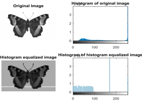
An image histogram provides a comprehensive description of an image. It represents the occurrence of different levels of gray relative to the frequencies. Like other histograms, the histogram of an image often displays frequency. But the frequency of pixel intensity values is shown by an image histogram. The equalization of the histogram is used to improve contrast. Contrast is not always going to be an increase. There may be some cases where the equalization of the histogram may be worse. The contrast is diminished in those situations. Figure 3.15 shows us plotting the histogram of the original image and the histogram-equalized image, using MATLAB commands we can use these types of butterfly image:
Histogram
There exist many applications of histograms in image processing. The first is the image's analysis. By looking at its histogram, we can predict an image. It's like searching for a piece of a body's x-ray. The other use of the histogram is for purposes of brightness. The histograms have broad image brightness applications. Not only in brightness but also in histograms are used to change a picture's contrast. The equalization of an image is another significant use of histograms. And last but not least, thresholding is widely used by the histogram. This is mostly used in the view of the machine.
Extracting and selecting features
Four characteristics of shape, texture, light, and vein are used in the conventional identification theory to distinguish different butterfly species. According to several studies, due to the colorful scales on the wings, it was discovered that the vein features were tough to acquire from the digital image of the butterflies. In fact, butterfly specimens would have different colors for the same species due to the different preservation period. But after the full metamorphosis, the form and texture of the butterfly wings are relatively stable. And the shape of different samples of similar species is less variable than the texture. In addition, there is a significant difference between different species in the shape of butterfly wings. The shape characteristics are therefore used for the identification of the basic level and the texture characteristics are used for further identification. There are many feature selection techniques that are now being used widely in these days, such as Convolutional Neural Networks (CNNs), Independent Component Analysis (ICA), Principal Component Analysis (PCA), and Linear Discriminant Analysis (LDA), this analysis will concentrate on Convolutional Neural Networks (CNN).
PART 4
ARTIFICIAL NEURAL NETWORK
Artificial neural network (ANN), which is a machine learning method, is a parallel computing system to mapping function from inputs to outputs. Basically, ANN includes mathematical nonlinear methods originated to perform accomplish the complex exercise. ANN is mimicked biological brain networks having the capability to the adaptation to nature, learning and recall of information. Over the years, ANN‟s being used in numerous fields of machine learning applications comprising image processing, identification, classification, optimization, power systems, signal processing, and control system.
Figure 4.1. shows the general overview of ANN which includes three types of layers namely, input, hidden and output. The input layer brings the initial data (input features or decision variables) into the system for further processing by subsequent layers of artificial neurons. The hidden layer is connected to the input and output layers. Each connection in this layer takes weight and produces output through an activation function. The output layer produces outputs of ANN.
An ANN is generally formed from multiple connected processing nodes called as artificial neurons and their connection between them. The network consists of seven major components:
1. Weighting Factors 2. Summation Function 3. Transfer Function 4. Scaling and Limiting 5. Output Function 6. Error Function 7. Learning Function.
A classical feed-forward multi-layer perceptron (MLP) architecture can be used for regression or classification tasks. It has two phases namely training and test. Generally, training and test phases use the same dataset which is divided into two groups. In the training phase, for a predetermined specific dataset, until the ANN reaches the desired accuracy, neuron‟s wights are upgraded. The accuracy of the architecture is proportional to the selected parameters and dataset. Thus, parameter optimization of ANN and the fine-grained datasets is essential. If the dataset has no enough samples to cover all its aspects, the accuracy of the network will reduce.
The training phase performs two ways supervised (labeled data) or unsupervised (unlabelled data). For supervised training of MLPs, one of the very general methods is the back-propagation algorithm. This algorithm is grounded on the gradient descent. The weights of the network are randomly initialized and then changed in a direction along the negative gradient of the mean squared error (MSE) so as to minimize the difference between the network output and the desired output.
The training of the network comprises four steps: (1) determining the training data, (2) design the ANN, (3) train the ANN lastly (4) determine the accuracy of the network outputs with the test dataset. After a determined step of the training process, the ANN will have an adequate ability to perform a nonlinear pattern association
between input and target. A well-trained network will effortlessly anticipate the output when a new input data is applied to it.
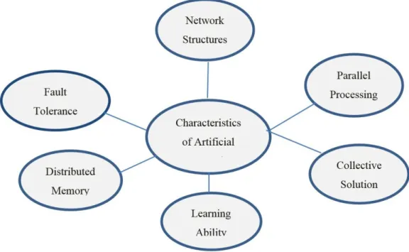
4.1. ANN CHARACTERISTICS
ANN Characteristics Mainly computers are good in calculations that mostly take input process and after which it provides the result based on calculations that are performed on different algorithms that are programmed in the application whilst ANN improves their own commands, the more decisions they make, the better decisions can be made. The network characteristics of ANN is given in Figure 4.2.
Figure 4.2. Artificial neural network characteristics.
4.2. NETWORK STRUCTURE
ANN's network configuration should be uncomplicated and straightforward. There exist primarily two types of recurring and non-recurring structures. Also known as the Auto Associative or Feedback Network is the Recurrent Structure and the Non-Recurrent Structure is also known as the Associative or Feed-forward Network. The signal travels in one direction only in the feed-forward network, and as for Feedback
Network, the signal travels both ways by adding loops into the network. Below are the particulars showing the way signals are fed-forward and feedback in both the network structures.
4.3. IMAGE DATA PRE-PROCESSING FOR NEURAL NETWORKS
In the past few years, deep learning has really entered the mainstream. Deep learning uses neural networks with many hidden layers (dozens in the state of the art of today) and requires large amounts of data from training. In perceptual tasks such as vision, voice, language processing, these models have been particularly effective in gaining insight and achieving human-level accuracy. Several decades ago, theoretical and mathematical foundations were laid. Two factors have led primarily to the growth of machine learning are
1. The availability of massive data sets/training examples in multiple domains and 2. Advancements in raw computing power and the rise of effective parallel
hardware.
The most common parameters of image data input are the number of images, the height of the image, the width of the image, the number of channels and the number of pixel rates.
PART 5
LITERATURE REVIEW
There are many studies in the literature related to insect classification and identification. In the last two decades, there has been a significant increase in the number of researches on neural networks due to the availability of fast computers and a large amount of data. Keanu Buschbacher et al. proposed a new approach called DeepABIS which is based on the Automated Bee Identification System (ABIS). ABIS that is a fully automated approach aims to recognize bee species from the pattern on their forewings. DeepABIS has three important features: (1) DeepABIS employs automated feature generation to reduce the efforts of training the system using convolutional neural networks (CNNs), (2) DeepABIS enables web portals and participatory sensing using mobile smartphones and a cloud-based platform for data collection, (3) DeepABIS is adaptable to other insects beyond bees, such as butterflies, flies, etc. DeepABIS achieved to identify wild bees on the ABIS dataset an average top-1 accuracy of 93.95% and a top-5 accuracy of 99.61%. They then adapted DeepABIS to a butterfly dataset including 5 classes and obtained classification results with an average top-1 accuracy of 96.72% and a top-5 accuracy of 99.99% [16].
Linan Feng et al. develops an automated moth species identification and retrieval system using computer vision image processing techniques. The system is a probabilistic model that infers attributes from visual features of moth images in the training set and learns the co-occurrence relationships of the attributes [17]. They tested their system on a dataset consisting of 4530 images of 50 moth species and estimated the best recognition accuracy of 70% for some species. The lowest accuracy they obtained is approximately 34% for species Narcus Burns. The main difference between their work and the other similar works for insect classification is that they provide intermediate-level features which are Semantically Related Visual
(SRV) attributes on moth wings such as eyespots, white central band, marginal cuticle, and snowflake mosaic.
Kaya et al. [3] proposed two different local binary patterns (LBP) descriptors for detecting special textures in images. The first one is based on the relations between the sequential neighbors of a center pixel with a specific distance and the other one is relies on determining the neighbors in the same orientation through the central pixel parameter. They tested their descriptors to identify butterfly species on lab-based images of 140 butterflies collected in Van city of Turkey. The highest accuracy they obtained for classifying butterflies by the artificial neural network is 95.71%. Kaya and Kaycı [4] developed a model for butterfly identification based on color and texture features by the artificial neural network using the gray level co-occurrence matrix with different angles and distances. The accuracy of their method reached 92.85%.
Wen and Guyer [5] developed a model which combines local and global features for insect classification via five well-known classifiers that are K nearest neighbor classifier (KNNC), normal densities based linear classifier (NDLC), minimum least-square linear classifier (MLSLC), nearest mean classifier (NMC) and decision tree (DT). Their experimental results tested on images collected from actual field trapping for training yielded the classification rate of 86.6%.
Xie et al. [6] improved a learning model for the classification of insect images using advanced multiple-task sparse representation and multiple-kernel learning techniques. They tested the proposed model on 24 common pest species of field crops and compared it with some recent methods.
Feng et al. [7] improved an insect species identification and retrieval system based on wing attributes of moth images. Their retrieval system is based on CBIR architecture which is not about having a final answer but just providing a match-list to the user. The final decision can be made by an expert.
Yao et al. [8] designed a model to automate rice pest identification using 156 features of pests. The authors tested the proposed model on a few species of Lepidoptera rice pests with middle size using the support vector machine classifier. Another study for pest detection and recognition was carried out by Faithpraise et al. using the k-means clustering algorithm and correspondence filters [9].
Leow et al. [10] developed an automated identification system of copepod specimens by extracting morphological features and using ANN. They used seven copepod features of 240 sample images and estimated an overall accuracy of 93.13%.
Zhu and Zhang [11] proposed a method to classify lepidopteran insect images by integrated region matching and dual-tree complex wavelet transform. They tested their method on a database consisting of 100 lepidopteran insects of 18 families and estimated the recognition accuracy of 84.47%.
Mayo and Watson [12] showed that data mining techniques could be effective for the recognition of insect species. They used WEKA which is a data mining tool with different classifiers such as Naïve Bayes, instance-based learning, random forests, decision trees, and support vector machines. WEKA was able to achieve an accuracy of 85% using support vector machines to classify live moths by species. Another work for identification of live moths was conducted by Watson et al. [13] who proposed an automated identification tool named DAISY by analyzing wing attributes and shapes. However, DAISY requires user interaction for image capture and segmentation.
Silva et al. [14] aimed to investigate the best combination of feature selection techniques and classifiers to identify honeybee subspecies. They found the best pair as the combination of Naïve Bayes classifier and the Correlation-Based feature selector in their experimental results among seven combinations of feature selectors and classifiers.
Wang et al. [15] designed an identification system of insect images at the order level. They extracted seven features from insect images. However, the authors manually
removed some attached to insects such as pins. Their method has been tested on 225 specimen images from 9 orders and sub-orders using an artificial neural network and 7 features with an accuracy of 93%. They achieved an accuracy of 92% using a support vector machine and 7 features.
Angelo et al. [18] created a mobile application for the Android platform for insect identification using the Inceptionv3 model, which is a convolutional neural network architecture. The Android application, named Insectify, provides offline functionalities to general users. 10 insects are considered in their study. These are butterfly, bee, beetle, cockroach, cicada, house fly, dragonfly, mantis, wasp, and grasshopper. They conducted the tests to assess the effectivity of the model on images with varying color mode, orientation, and background. The model achieved a maximum accuracy of 95.33% based on the model's first guess of the correct insect common name. The model was able to isolate distinct features in an image captured by mobile phones. Therefore, Insectify may be a useful and portable tool to provide insect identification beneficial to different fields of studies and localities such as farmlands, forests and common households.
Xue et al. proposed a new model to identify butterfly species [19]. Their model includes two significant improvements: extracting the gray-level co-occurrence matrix (GLCM) features in image blocks and weight-based k-nearest neighbor (KNN). The model they improved extracts GLCM features from three image blocks of butterfly images. They do not work on the whole butterfly area. Because extracting GLCM features on the whole area will increase the running time and some important features in the local area will be ignored. After computing GLCM features, they used a weight-based KNN search algorithm for classification. The identification accuracy of their method for 10 butterfly species reached 98%.
PART 6
METHODOLOGY
In this thesis, our study consists of two stages. In the first stage, we studied on lab-based butterfly images taken on under a fixed protocol. The species of butterflies in these images are identified by expert entomologists. We used a total of 140 images taken in [20] for lab-based butterfly images of 10 species. After applying some preprocess to the images such as histogram equalization and background removing, we extracted several features from the butterfly images. Finally, we used an artificial neural network in MATLAB version R2014b using the Neural Network Toolbox for butterfly identification. The ANN model could achieve an accuracy of 96.5% using one input layer, one hidden layer, and one output layer. The details for the model used and the other information are given in the following sections.
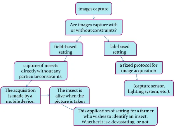
In the second stage of the thesis, we studied on field-based butterfly images. Field-based images of butterflies are taken in nature without any protocol or constraints. These pictures are generally taken using either a mobile device or a digital camera. We gathered 44659 images of 104 species from the website of Butterflies Monitoring & Photography Society of Turkey that consists of field-based butterfly images [20]. To identify the species of the field-based butterfly images, Convolutional Neural Networks which is a class of deep learning was used. Each class was divided into two parts automatically: the training part (80%) and the testing part (20%). Approximately 80% of success was achieved for both test and training data using CNN architecture.
Figure 6.1. Flowchart to explain the research methodology.
6.1. ADVANTAGES AND DISADVANTAGES
According to the common use of mobile devices, field capture is very easy. A lot of users can take butterfly photos in nature. These photos do not require any special hardware and a fixed protocol such as the position of butterflies, the shooting angle, butterfly distance, occlusion, lighting, and background complexity. Therefore, researchers can collect many sample images by themselves or from the internet to construct a dataset of butterflies. However, identification systems working on field-based images are difficult to design and do not generally yield good accuracy.
Collecting the lab-based butterfly dataset is difficult, because it needs a fixed protocol, identifying them is time-consuming work for entomologists, and the number of butterflies included in the butterfly dataset is not comprehensive. However, preprocessing operations such as background removing is quite easy. Therefore, machine learning techniques for classification give more accurate results.
6.2. FOREGROUND / BACKGROUND DETECTION
Before related features are extracted, the system needs to know which region of the image is important. This part is taken care of by segmentation. In some cases, segmentation is learned in a supervised manner as in [60, 61]. The study in [61] feeds the whole image to the classifier, which is supposed to learn to discriminate only on the foreground and therefore to recognize it. The approach in [60] is based on learning on both negative and positive sample images. Negative sample images are images where there is no any insect but only foreground. Learning on such images enables the system to ignore the background. When segmentation is irrelevant, it may be asked to the user. The user can select the region of interest on the given interface by drawing its outlines. However, manual segmentation might be a tedious and time-consuming task considering how numerous the images can get. That is why segmentation is worth automated most of the time.
Some segmentation techniques are based on thresholding which is basically splitting the image histogram into several groups that correspond respectively to the object and the background. The simplest way of performing thresholding is to set the intensity value that separates these two groups. The intensity value can be set statically in the program or by the user who can select the one which gives the best result as in [22,23]. Another way of performing thresholding is to see it as a clustering problem where two or more clusters (which are the regions) have to be formed [24-27].
Otsu's method criterion is about choosing the clusters such that the intra-cluster variation is minimized while the inter-cluster one is maximized [10,25,27]. k-means is used onto the color space to search for centroids representing the different regions in the image based on color similarity [9,26]. The study in [9] uses ISODATA, a clustering algorithm that builds clusters with a given standard deviation threshold. The studies in [10,27] use mean shift clustering in the color space as a preprocessing step to Otsu.
There are other techniques to segment objects from the images. The papers in [28,29] use active contours (snake) that take a simple thresholding mask as a seed point to get a more accurate segmentation. The work in [7] uses background segmentation (which implies the background to be constant). The study in [30] supposed the object in the image gives the longest outline while the research in [6] searches for lines on wing images and uses the symmetry of Lepidoptera as a detection criterion.
6.3. MATERIALS
6.3.1. Dataset
The number of butterfly species in the world varies from 15000 to 21000 according to a recent estimate in [1]. In this thesis, we studied two types of images, field-based images, and lab-based images.
6.3.1.1. Field-Based Images
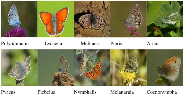
We gathered 44659 images in different 104 classes from the website of Butterflies Monitoring & Photography Society of Turkey [20]. When images were downloaded from the website, we labeled the species which were approved by professionals. The dataset was divided into 104 different classes using these information labels. Since many classes have a few image samples, we restricted it to include 10 classes with the most sample size as shown in Table 6.1. The new dataset has 17.769 images. The number of classes has been reduced to 10 in order to increase the classification accuracy and to remove the classes with fewer samples. Since all images on the website are of different resolutions, they were resized to 224x224 pixels. Sample images for each class are given in Figure 6.2. Since the input images were captured from wide field-of-view cameras, they have some characteristics such as occlusion and background complexity.
Table 6.1. Name and the number of images per butterfly‟s genus in the dataset. Genus Images Polyommatus 5559 Lycaena 2472 Melitaea 2235 Pieris 1530 Aricia 1080 Pyrgus 1036 Plebejus 1003 Nymphalis 989 Melanargia 943 Coenonympha 922
Polyommatus Lycaena Melitaea Pieris Aricia
Pyrgus Plebejus Nymphalis Melanargia Coenonympha
Figure 6.2. Sample images in the field-based dataset.
6.3.1.2. Lab-Based Images
We used images of 140 specimens from 14 butterfly species (see Figure 6.3). For each species, there were 14 specimens.
Figure 6.3. Lab based butterfly images with 14 butterfly species.
6.3.2. Image Preprocessing Step
The preprocessing procedure to segment the butterfly from the input image consists of seven steps. They are shown in Figure 6.4.
Arethusan Chazara anthe Chazara bischoffi Chazara briseis
Hipparchia statilinus
Melanargia hylata Melanargia russiae Melanargia syriaca
Psedochozara beroe
Satyrus favonius Psedochozara pelopea
Pseudochazara geyeri
Figure 6.4. Image preprocessing steps.
6.3.3. Implementation
We implemented image preprocessing steps on Python according to Figure 6.4. The python script is shown in Figure 6.5.
Figure 6.5. Python script of the preprocessing step.
6.3.4. Explanation of The Script
In line 1, we import numpy package for scientific computing
In line 2, we import OpenCv package for image processing
In line 3, we import Pyplot module. Pyplot is a matplotlib module which provides a MATLAB-like interface to plot figures.
In line 5, we read the input butterfly image as img.
In line 11, The cvtColor function in OpenCv is the function that performs transitions between color spaces. The COLOR_BGR2LAB parameter is used to convert from BGR to LAB (CIE). As another parameter, the cvtColor function retrieves the desired (img) display object to be converted. The transformed image object named img is assigned to the image object named Lab. Color spaces in OpenCv are represented by 3-Dimensional bands.
In line 12, cv2.split function in OpenCv splits the image to Bands of the color spaces. It takes the image object (Lab variable) to be separated into bands as a parameter. The bands of Lab image space are a-Dimension, Luminance, and b-Dimension. The bands that are separated here are assigned to variables named a-dim, luminance and b-dim.
In line 14, a band is a 2-dimensional array. To use for the next computations and to solve the array size mismatch problem, a 3-band temporary image object is created using the only a-dim band of the above image.
In line 16 and 17, the image must be a grayscale image for thresholding. Since there is no conversion from LAB color space to grayscale, we first convert the image to BGR, then convert the resulting image to grayscale.
In line 19, we use a function named cv.threshold for thresholding. The first argument is the source image that must be a grayscale image. We already obtained the grayscale image in line 17. The second argument is the threshold value which is used to classify the pixel values. The third argument is the maxVal which represents the value to be given if the pixel value is more than (sometimes less than) the threshold value. OpenCV provides different styles of thresholding and it is decided by the fourth parameter of the function. We use the Otsu algorithm to find the optimal threshold value. Inverse binary thresholding (cv2.THRESH_BINARY_INV) is just the opposite of binary thresholding. The destination pixel is set to zero if the
corresponding source pixel is greater than the threshold value and to max value, if the source pixel is less than the threshold. The formula is as follows:
(6.1)
In lines 22 and 23, we smooth the image in order to reduce noise. The median filter replaces each pixel with the median of its neighboring pixels (located in a square neighborhood around the evaluated pixel). The size of the median filter is 3x3. We also use the functional morphology to apply Morphological Transformation such as opening, closing, morphological gradient, etc. we performed the closing operation. It is useful to remove small holes (dark regions). After the execution of this line, the image object called median was obtained. In line 26, the unwanted pixels obtained after the threshold process which cannot be removed by the median filter have been removed with the dilate morphological function in OpenCv. Dilation is the opposite of erosion. Generally, in cases like noise removal, erosion is followed by dilation. Because, erosion removes white noises, but it also shrinks the object. Therefore, we dilate it. Since noise is gone, they won’t come back, but our object area increases. It is also useful in joining broken parts of an object.
In line 29, function connectedComponentsWithStats retrieves useful statistics about each connected component. After dilation in the previous operation, in line 26, we may have several components in the image. We are interested in the biggest object which is ROI (region of interest). Image with 4 or 8-way connectivity - returns N, the total number of labels [0, N-1] where 0 represents the background label. In our segmentation, we used 4 connectivity. If the 4-pixel neighborhood is similar to the other 4 pixels, which is a neighbor to a pixel, then we have considered it to be a component of the object.
In line 32, we define the pixel number of the smallest object as 100000 pixels by experimental tests.
In line 33, num, zeros return a new array of given shape and type, filled with zeros. That is a black image.
In lines 35-37, All the objects are compared with each other and the small ones are excluded. and as a result, a mask that specifies only for the object to be segmented in the image variable named img2 is obtained.
In line 43, we perform LOGICAL AND operation between the original image and img2 which is desired to be segmented that is found in the above loop. The function bitwise_and calculates the per-element bit-wise logical conjunction when two images have the same size.
In line 46, the show displays the image, write saves image data to the file specified by filename.
In line 48, the pyplot class of the matplotlib library which is imported in line 15 is used below begins with plt. The desired image to be shown is given to the subplots as the parameter respectively.
6.4. EXPERIMENTAL TESTS
6.4.1. Field-Based Images
The segmentation process performs well for some field-based images. However, if the background contains nature objects, such as flowers, stones, leaves, etc. then our script cannot make segmentation very well. Another reason is the light and the color of the butterflies. Some examples for successful and unsuccessful segmentations are shown in Figure 6.6 and 6.7, respectively.
Figure 6.7. Unsuccessful segmentations.
6.4.2. Lab-Based Images
We use different color transformation in lab-based images. The following statements are replaced instead of lines 11,12,14,16,17 of field-based python code, respectively. Here, we use the HSV color space instead of the CIE-Lab color space.
Hsv= cv2.cvtColor(img, cv2.COLOR_BGR2HSV) Hue,Sat,Val = cv2.split(Hsv)
tmpHsv=cv2.merge([Sat,Sat,Sat])
tmpHsv= cv2.cvtColor(tmpHsv, cv2.COLOR_HSV2BGR) HsvGray=cv2.cvtColor(tmpHsv, cv2.COLOR_BGR2GRAY)
The results of all image preprocessing steps are shown in Figure 6.4 are illustrated in Figure 6.8. We show some successful segmentation of lab-based butterfly images in Figure 6.9.
Figure 6.8. All steps of the segmentation.
Chazara anthe
Chazara briseis
Hipparchia statilinus
Psedochozara beroe
Psedochozara pelopea
PART 7
LOCAL BINARY PATTERN
Local binary patterns (LBP) [30] represent one prominent texture descriptor that has shown effective results in computer vision applications. Their histogram can be used as a powerful local pattern descriptor. These local patterns describe micro-structures (e.g., edges, corners, flat region) and their underlying distribution is estimated by the histogram. The histogram of the image represents local structures extracted from the entire image by combining both structural and statistical information. Figure 7.1 shows an example for evaluating the feature histogram representing the butterfly image where the butterfly image is represented by concatenating a set of local LBP histograms. The success of the LBP in these applications motivated us to utilize it in the butterfly recognition problem. There are a number of the LBP variants proposed recently for specific problems.
Figure 7.1. The steps for obtaining the final feature histogram representation using LBP.
7.1. THE BASIC LBP
The basic LBP operator was introduced by M. Pietikäinen [31] which characterizes the spatial structures of local texture patterns in images using a 3×3 square patch around a central pixel as illustrated in Figure 7.2. The LBP is defined as a set of binary comparisons of pixels intensities between the center pixel and its eight