A comparison of hazard rate estimators for left truncated and right censored data

Printed in Great Britain

A comparison of hazard rate estimators for left truncated and

right censored data

BY ULKU UZUNOGULLARI

Faculty of Industrial Engineering, Bilkent University, Ankara, Turkey

AND JANE-LING WANG

Division of Statistics, University of California, Davis, California 95616-8705, U.S.A. SUMMARY

Left truncation and right censoring arise frequently in practice for life data. This paper is concerned with the estimation of the hazard rate function for such data. Two types of nonparametric estimators based on kernel smoothing methods are considered. The first one is obtained by convolving a kernel with a cumulative hazard estimator. The second one is in the form of a ratio of two statistics. Local properties including consistency, asymptotic normality and mean squared error expressions are presented for both estimators. These properties facilitate locally adaptive bandwidth choice. The two types of estimators are then compared based on their theoretical and empirical performances. The effect of overlooking the truncation factor is demonstrated through the Channing House data.

Some key words: Consistency; Kernel estimator; Mean squared error; Optimal bandwidth; Weak convergence.

1. INTRODUCTION

In medical follow-up or in engineering life testing studies one may not be able to observe the variable of interest, referred to hereafter as the lifetime. Among the different forms in which incomplete data appear, right censoring and left truncation are two common ones. Left truncation may occur if the time origin of the lifetime precedes the time origin of the study. Only subjects that fail after the start of the study are being followed, otherwise they are left truncated. Those that are followed are further subject to right censoring during the follow-up period. Left truncation and right censoring may thus arise together. See for example, an AIDS study by Struthers & Farewell (1989) where the 'lifetime' is the incubation period, and the truncation variable is the time from infection until the entry to the study.

Formally, let X be the random variable of interest, called the lifetime variable, with continuous distribution function F(x) = pr (X - x). Let T and C be the random variables for the left truncation and right censoring time respectively. It is assumed that T, C, X, are independent and, without loss of generality, that they are nonnegative. Let Y=

X A C min (X, C) and 8 = _I(Y = _{X), where I(.) is the indicator function. Under}

the left truncation and right censoring model one observes the triplets (Y, T, 8) only if T - Y, otherwise nothing is observed. The observations are thus taken from the conditional distribution of (Y, T, 8) given that T - Y Note that the above reduces to the right censoring model when pr (T = 0) = 1 and to the left truncation model when pr (C =+X) =1.

298 ULKO UZUNOGULLARI AND JANE-LING WANG

The nonparametric product-limit estimator of F for left truncated and right censored data was given by Tsai, Jewell & Wang (1987) and shown to be the nonparametric maximum likelihood estimator of F by Wang (1987). Our focus in the present paper is to estimate the hazard rate A(x) defined by A(x) =f(x)/{1 - F(x)}, where f is the probability density function of F. The left truncation factor is sometimes overlooked by researchers. This will result in underestimating the hazard rate as demonstrated in ? 7, Fig. 5, using the Channing House data of Hyde (1977).

The nonparametric estimation of the hazard rates was initiated by Watson & Leadbetter (1964) who proposed three types of estimators for independent and identically distributed observations. Two of these types are shown to be equivalent by Rice & Rosenblatt (1976). We extend both remaining types of estimators in ? 2 to accommodate left truncated and right censored data. The first type aims at estimating both the hazard function and its derivatives, and is constructed by convolving a kernel with a cumulative hazard estimator; see (2 8). The second type aims only at the hazard function itself and is in the form of the ratio of a kernel subdensity estimator and an empirical function; see (2 12).

Local properties of both types of estimators are studied in ?? 3 and 4 including consistency, asymptotic normality and mean squared error expressions. The derivation of the mean squared error for the ratio estimator, i.e. the second one, is nonstandard for kernel estimators. The optimal bandwidth which minimizes the leading term of the mean squared error is derived for both types of estimators. In particular, the optimal bandwidth for the ratio estimator is the same as the optimal bandwidth of the kernel subdensity estimator in the numerator. The kernel estimator which employs the optimal bandwidth is called the optimal kernel estimator. It is shown in Theorems 3 3 and 4 3 that the kernel hazard estimator employing a bandwidth which is a consistent estimator of the optimal bandwidth has the same limiting distributing as the optimal kernel estimator. This is referred to as locally adaptive bandwidth choice. Choices of consistent bandwidth estimators are suggested for both types of estimators.

The choice of bandwidths is crucial for the quality of the resulting kernel curve estimator. This is even more so for hazard rate estimation than for density estimation since the variance of the kernel estimator for the former tends to infinity for large values of lifetime. The truncation and censoring scheme further complicate the situation; in particular, both the bias and variance may blow up near both tails; see equations (3-6), (41) and (4-2).

The two types of estimators are then compared in ? 5. They have approximately the same variance but different biases. The ratio estimators usually yield very jagged curves unless a smooth empirical function is employed for the denominator. The global perform- ance of the locally adaptive bandwidth choices is compared to that of a fixed global bandwidth and the optimal bandwidth through a simulated sample in ? 6. The procedures are applied in ? 7 to the Channing House data given by Hyde (1977).

Our results in ? 4 extend some of the earlier results for right censored data by Ramlau-Hansen (1983), Tanner & Wong (1983), Yandell (1983) and Muller & Wang (1990). As for truncated data, except for a technical report by the authors and a Ph.D. dissertation by the first author, there are no published results on hazard function estimation to our knowledge.

2. DERIVATIONS OF THE TWO HAZARD ESTIMATORS

Refer to the left truncation and right censoring model in ? 1. Let (1<,, T,, 8,) (i = 1, .. ., n) be the independent and identically distributed random vectors which one observes, where

Yi = Xi A Ci, Si = I( Yi = Xi), Ti S Yi and Xi, Ci, Ti are independent with marginal distribu- tions F, H and G respectively. For any function K with values in [0, 1] denote K(t) =

1 - K (t). Under the independence assumption, the distribution function W of Yi satisfies W = HF. Note that the number of observations n is a random variable. All the arguments hereafter in this paper are conditional on n.

If K is a distribution function, let aK = inf {t: K(t) > O} and bK = sup {t: K(t) < 1} be

the lower and upper endpoint of support of K. Then under the current model, as discussed by Woodroofe (1985), one can expect to estimate F(x) only if

aG - aw = min (aF, aH), bG bw = min (bF, bH).

Otherwise only the conditional distribution FXI(x) = F(x I X ` T) can be estimated, for any T B _{aG. Note, however, that A(x) is always identifiable for x} T X, since AxI,(x) = A(x),

for x ? T. Therefore we do not need to be concerned with the identifiability problem in this paper. Assume that a = pr (T - Y)> 0. The subdistribution function W*1 (t) of the uncensored observations is

W*(y)=pr (Y y, 8 = 1I T Y)

= a-{{ f

_{G(x) dF(x) dH(s)+H(y-)}

_{G(x) dF(x)}.}

Hence

dW*(y) = a- G(y)H(y-) dF(y). (2<1)

Next, define

C(z) = pr _(T-- z -,--

YI

From (2.1) and (2.2), it follows that

dW*(z)/C(z) = dF(z)/F(z-) = A(z) dz, (2 3)

and the cumulative hazard function A is therefore

A(z)

A(t) dt =7

0 o ~C (t)

Let W*1 and Cn be the empirical estimators of W* and C respectively. Then n W*n( y) = n-1 I( Yi --- y, Si = l), (2 5) i=l n Cn(z) = n _E _{I (Ti ---z ---Y,} (2-6) i=l

Note here that nCCn ( Y1) ? 1 for i = 1, . . ., n. Replacing W* and C in (2 4) by their empirical counterparts one can estimate A(z) by

An

A-n (Z) =EI ( Yi --- Y, Si =

l

i=l

This estimator (2s7) is the cumulative hazard function of the product limit estimator of F given by Tsai, Jewell & Wang (1987).

300 ULKU UZUNOGULLARI AND JANE-LING WANG

Since one of our goals is to derive a locally adaptive estimator for A(z) and this involves estimating higher derivatives of A(z), we will present the results for the rth derivative A(r)(z) of A(z), for r ? 0. We consider the following kernel estimator for A(r)(x) by

convolving Krb(X) = b(r?l)Kr(x/b) with

An

r _A

n

Ak (z)

-Krb(z-u)

i=l

where Kr is the kernel and b = bn is the bandwidth. The subscript n is obviously suppressed

in k(r) for simplicity.

We will use a kernel function with the following properties.

Property 1. We have that Kr is in L2([-1, 1]) with support [-1, 1] and is of bounded variation.

Property 2. For some p - r,

(_l)r

ri

( j = r),

IXjKr(X) dX 0 (OSj<p, j *r),

finite but nonzero (j = p).

Note that, for p > 2, Property 2 requires kernels with negative values and that Kr depends on p implicitly. Such a kernel is said to be of order (r, p).

For the bandwidth we require the usual conditions,

b ->0 nb2r+l1 -o. (2*9)

An alternative estimator for A(z) can be obtained via (2-3) by estimating the subdensity w*(z) = dWW*(z)/dz and C(z) separately. Specifically, let K = Ko be a kernel function satisfying Property 1 and Property 2, and b = bn be the corresponding bandwidth sequence. Then a kernel estimator of w*(z) can be obtained by convolving Kb(x) = Ko,b(x)=

V-K(x/b) with W*, in (2 5) for a bandwidth b satisfying (2 9) with r=0:

{

n

w* (z) = Kb(z -u) dW* (u) = n E iKb(z Yi). (2*10)

J ~~~~~~~~i=1

To estimate C(z) the empirical function

Cn(z)

Y(n) is the largest order statistic of the Y's. There are several ways to modify

_Cn,

Cn(z)

Cn(Yi)

A _{fC(Z) if Cn(z)>0(}

where kn -0 as n-co.

An alternative estimator for A(z) is thus available by combining (2 10), (2 11) and this yields

Hazard rate estimators for left truncation and right censoring 301 Unlike (2-8) there is no need to estimate the rth derivative of A(z) for locally adaptive bandwidth choices for I since the optimal bandwidth requires estimation of w 2)(z) but not that of A(2)(z); see (3-7).

Properties of the estimators A(z) and A(r)(z) will be studied in ?? 3 and 4 respectively for aG < z < bw.

3. PROPERTIES OF A(z) AND LOCALLY ADAPTIVE BANDWIDTH

We show in this section properties, including consistency and asymptotic normality of X(z) in (2-12), for z such that aG<z<bw. Notice that 0<C(z)<1 on this range. These properties are then applied to obtain locally adaptive bandwidths. An estimator similar to I was studied by Blum & Susarla (1980) for its global behaviour under the right censoring model. We are mainly concerned with the local behaviour in this paper and our approach is different from theirs.

We first concentrate on estimating the rth derivative w*(r) of w*. To this goal we need to assume that, for some p ? r, w* is p times continuously differentiable at z. Let Kr be a kernel of order (r, p) satisfying Properties 1 and 2, and b be the bandwidth sequence satisfying (2 9). Denote

Brp (-1)P(p!)-' xPKr(x) dx, Vrp=j| K2(x) dx. (3.1) Recall that the kernel estimator for _w,(r) i

n

(z)

(z -y)

=

i=l

It follows from standard results on kernel density estimators based on independent and identically distributed observations that,

bias {W*(r)(z)}= bP rW(P)(z)Br,p + o(bPr), p> r (3-3) var {wI( )(z)}=(nb2r+l)lw*(z) V + o{(nb2r+l)l}(34)

Hence, letting

d = lim nb2p+I < o, (3*5)

n --oo

it follows that (nb2r+l) {w,(r)(z) - W*r)(z)} converges in distribution to

N(dlw*(P)Brp W*(Z) Vrp).

Next notice that pr (Cn(z)= 0)={1-C(z)}n =Cn(z). Hence (2411) implies that

Cn(z) - _Cn(z) = _op(n-2) and thus Cn(z) - C(z) = _{Op(n-). The consistency and asymptotic}

normality of A(z) thus follow by setting r = 0.

THEOREM 3-1. (a) We have that X(z) is a consistent estimator of A(z). (b) We also have that (nb)1{X(z) - _{A(z)} converges in distribution to}

N (d 1{w (P) (z) / C (z)}IBoP pI {A(z) / C (z)}I VO p).

The actual bias and variance expressions of A require some calculations which are postponed to the Appendix.

302 ULKU UZUNOGULLARI AND JANE-LING WANG THEOREM 3-2. For p B 1, the mean squared error of X(z) is

MSEA(z)l= _ C(z)

Vo,p + b2pt C(z) _{BO'p +( o} b2P (3 6)

IV1L~ '~V/Jnb C (z) ' C(z)

0J*

where the first and second terms are respectively, the leading term of the variance and the square of the bias of X(z). The optimal bandwidth which minimizes the leading terms in MSE {Xk(z)} above is

n/(2p+) w*(z) VP }12]/(2p+l)

b'(z) =

n

2p f w (P (z

JOP

(3-7)

The mean squared error expression in (3 6) is a stronger result than the usual asymptotic mean squared error dealt with in the literature for a ratio estimator. The proof of Theorem 3-2 in the Appendix can be adopted almost verbatim to improve some results in the

literature. The optimal rate of the bandwidth

is the same as the usual kernel

density estimator for independent and identically distributed observations. Note that b'(z) in (3.7) is also the optimal bandwidth for the kernel estimator Of of w* and it depends on unknown quantities w*(z) and w*(P)(z). The next theorem shows that any consistent estimator 8(z) of 8'(z) yields a locally adaptive bandwidth.

Let w(z, [3 ) = w*{z; p(z)} and

A(z; ,3) = A{z; /(z)} (3 8)

denote respectively the estimator (24 10) and (2s 12) with bandwidth b

=

Choose 8a and P8b such that 0 < Pa <p'(Z) <P,b < 00 and define the following bandwidth process for Pa 1 P P3b

- _{nP/(2P+l){ W*(z;} f) _w)*(z)}. -

Standard arguments for locally adaptive bandwidth choice based on independent and identically distributed observations (Abramson, 1982; Krieger & Pickands, 1981) show that the process {4n(,()} converges weakly on C[,Pa, Pb] to a Gaussian process. This then implies that

,8 (/z)) - _{'n{ (z)} - nP/C2P+1} (z)[A{z; 8 (z)} -A {z; '(z)}]

tends to zero in probability provided p(z) tends to 8'(z) in probability. Since Cn -> _C(z)

in probability we obtain that

nP/(2P+1)[i{z; / (z)} - _{{z; X'(z)}]}

tends to zero in probability. Slutsky's theorem and Theorem 3* 1 thus imply the following.

THEOREM 3*3. Assume p> rand that the kernel

K,

on the real line. Then for any consistent estimator 1(z) of ,'(z) the limiting distribution of

n +1.(z; f

P)

are the same and is the normal distribution with mean {p8(z)}P{w*(P)(z)1C(z)}B(,p and variance [,P'(z)]-7[A(z)/ C(z)] VO,p.

Remark 1. A consistent estimator of 8'(z) can be obtained by estimating w* and w*(P) consistently at z. For r = 0 and p, the kernel estimators in (3 2), denoted respectively by

W._o(z) and w*(iP)(z) to indicate that they are initial estimators, are indeed consistent. It should be noted that the initial kernels for iw*O and I*(P) are Ko and Kp respectively.

The initial bandwidth bdp for A *(p) _{should be larger than the initial bandwidth bdo for} wi0(z), with n

bdo

-cx)

>o.

A candidate for ,8(z) in Theorem 3-3 is thus

[3(z) = [ *o(Z) _voB,

1

4. PROPERTIES OF A( )(Z) AND LOCALLY ADAPTIVE BANDWIDTH

In this section we present similar results as in ? 3 for the estimator A(r)(z) in (2 8). To proceed, we first draw the attention of the readers to the analogy between the estimator

A(r) in (2.8) and an estimator in an unpublished report of the authors for left truncated data only. Both estimators aim at A(r)(z) and bear similar form except for different estimators of C and the indicator 8 appearing in (2 8) to account for the censoring effect. This similarity allows the results under left truncation to be adapted to our estimator (2-8). Details of the proofs are therefore omitted in this section and referred to the above article.

We assume, for p > r, that A is p times continuously differentiable at z and restrict our attention to aG < z < b, as in ? 3.

THEOREM 441. (a) Forp > r,

bias {A(r)(z)} - _{bPrA(P)(z)Brp + o(bP-r). (44)} (b) If C is continuous at z, then

nb2r+l var {A(r)(z)} = {A(z)/ C(z)} Vrp + o(1). (4 2) (c) Suppose C is continuous at z, then A(r)(z) is a consistent estimator of A(r)(z). The asymptotic normality of A(r)(z) is established via its Hajek projection.

THEOREM 4-2. Suppose C is continuous at z and d = lim nb2p+1 < oo. Then

(nb2r+l) {(r)(z) -A(r)(z)} - _{N(d"A(P)(z)Br,p, {A(z)/ C(z)} Vr,p). (4-3)} We will now consider the local bandwidth choice. It follows from (4.1) and (4 2) that

the optimal bandwidth b*(z) which minimizes the leading term of MSE {A(r)(z)} is b*(z) - 1/(2p+1) [2r+1 A(z) Vrz) 11/(2p+1)

L2( p-r)

A(

_n 1-/+l)/3*(Z) (4*4)

The optimal bandwidth depends on the unknown quantities A(z), C(z) and A(P)(z). Theorem 4 3 states that any consistent estimator ,8(z) of ,8*(z) will yield a locally adaptive bandwidth. The proof is omitted. Let

A(r)(z; /3) _{= A(r){z; A3(z)}} (4*5)

be the kernel estimator (2 8) with bandwidth b = n-11(2p+l) 8(z), and

Un (,!3 ) = n(P-r)/(2P+l){A(r)(z; /3) - A(r)(Z)}

THEOREM 4-3. Suppose C is continuous at z, p > r, and the kernel Kr is Lipschitz of order

a >2 on the real line. Thenfor any consistent estimator,3 (z) of,8*(z) the limiting distributions

of Un(/!3(z)) and U1(, 3*(z)) are both normal with mean {/3*(z)}PrA(P)(z)Brp and variance {/3*(z)}-(2r+l){A(z)/ C(z)} Vr,p-

304 ULKO UZUNOGULLARI AND JANE-LING WANG

Let Xo(z) and A(P) (z) denote the initial kernel estimators according to (2-8) for r =0 and p respectively, and let CQ(z) be as given in (2 11). A candidate for ,B(z) in Theorem 4-3 is

A =

[2r+ 1

o(z)

5. COMPARISONS OF THE TWO TYPES OF ESTIMATORS

Let A(z) denote the estimator A(r)(z) in (2 8) with r= 0. We compare it in this section with the other estimator A(z) in (2 12). The comparison will first be made on the theoretical framework as laid out in ?? 3 and 4. In ? 6 they will be compared on practical performance based on simulated samples. Comments similar to those in this section are also made independently by Patil, Wells & Marron (1991) for independent and identically distributed samples.

First, the variances of the two estimators are asymptotically equivalent but they differ in the biases; see (3*6) and (4 2). Since C(z) tends to zero as z approaches aG or bw the variances of both estimators tend to infinity as z tends to aG or bw.

Secondly, when a fixed bandwidth is employed, the assumptions on F, G and H for properties like consistency and asymptotic normality, centred at the expected value of the estimator, are similar for both estimators. For the adaptive bandwidths in (4 6) with p =A2,

(z,

Thirdly, the estimator

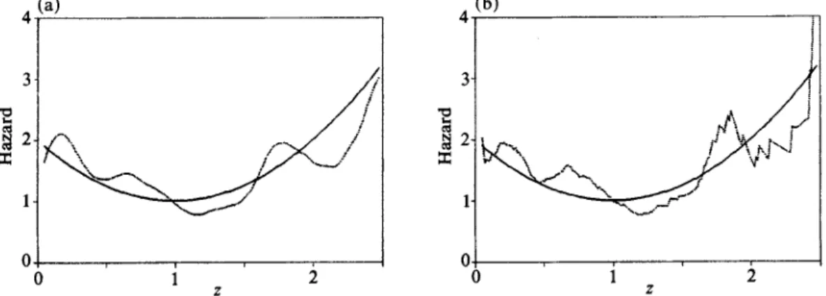
X

Fourthly, when adaptive bandwidths are employed, the initial bandwidths have to be chosen with some care. In reality the initial bandwidths can be determined by a global procedure if such a procedure is available or subjectively by inspecting the range and spread of the data and the location of the point z. Once a bandwidth is chosen one can

(a) (b)

z z

Fig. 1. (a) Dotted line, estimator A(z) in (2.8) with fixed bandwidth b = Ot3; solid line, true curve. (b) Dotted line, estimator X(z) in (2.12) with fixed bandwidth b = O3; solid line, true curve.

either use it as the initial bandwidth for the adaptive procedure or iterate the adaptive procedures a few times, starting with this bandwidth, to produce another initial bandwidth. As mentioned earlier, the initial bandwidths for A(2) and w*(2) should be larger than those for A and wt*.

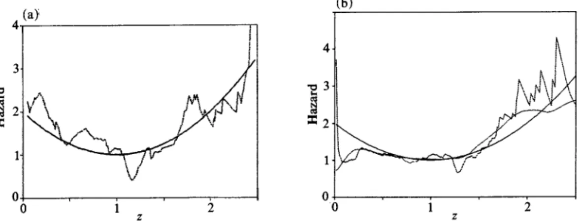
Fifthly, the locally adaptive estimators when applied over a range of z's usually yield spikes at several points; see Fig. 2(a). This can be corrected as suggested by Muller (1988, p. 120) and Schucany (1989). Further discussion is given in the next section.

6.

We demonstrate in this section how to apply the adaptive procedures of ?? 3 and 4 in practice and compare their global performance through simulated samples.

The lifetime variable is simulated from a distribution F with hazard rate A(z)=

(Z _1)2+ 1. This failure rate is chosen so that it has a bowl shape which would resemble

most practical life distributions. The constant 1 is added to avoid A being zero at z = ₁

which distorts the optimal bandwidth expression for X(z). Note that the bowl shape of this hazard function A makes it harder to estimate near both the left and right boundaries as opposed to a hazard function which tails off to zero at either boundary.

Both the censoring and truncation distributions are simulated from exponential distri- butions with means 4 and 0 1 respectively. A random sample (Xi, Ci, T1) of size 200 is simulated independently. This resulted in a censoring proportion of 14-8% for the Y data and a truncation proportion of 17% for the (Y, T) data. The observed sample size n is equal to 166. For estimating A(z) and w*(z), the kernel

KO(x)=

+x

of order r =0, p =2 is used. To estimate A(2)(z) and w*(2)(z) the kernel, K2(x) =315(-_1 + 9X2 _ 15x4

+

of order r =2, p =4 is employed. Both kernels are chosen with reference to Miuller (1988, p. 68) as they have certain optimality properties. Note also that both Ko and K2 above are Lipschitz continuous of order one on (-oo, oo), hence are appropriate for the adaptive bandwidth choice.

A global fixed bandwidth bdo = 03 is chosen for both A(z) and A(z) for all 0<

z

For the adaptive bandwidth estimator we use A(z, ,B) with 13 given in (4 6). Global initial bandwidths bdo=0 3 and bd2 =0 7 are used for

k(z)

13

b*

resulting truncated adaptive bandwidth estimator is plotted in Fig. 3(a). This corrects the spikes but not the left boundary problem. Further research on boundary modification is needed; see, for example, Rice (1984). The theoretical optimal bandwidth estimator is plotted in Fig. 3(b) for the purpose of comparison. The optimal kernel estimator has

306 ULKO UZUNOGULLARI AND JANE-LING WANG (a) (b) 4i 4- 3- 3- 2 0 1 2 z z

Fig. 2. (a) Dotted line, adaptive estimator k(z, f3) in (4.5) with f3 in (4.6); initial bandwidths, bdo = 0 3, bd2 = 0 7; solid line, true curve. (b) Adaptive bandwidth b corresponding to Fig. 2(a).

4(a) (b)

0 2 :0 1 2

z z

Fig. 3. (a) Dotted line, adaptive estimator in Fig. 2(a) with adaptive bandwidth truncated below at 0 15 and above at 06; solid line, true curve. (b) Dotted line, theoretical optimal bandwidth estimator

with b*(z) in (4.4); solid line, true curve.

(a)

(b

4-~~~~~~~~~~~~~~~~~~~~~~~~~~I

0

~ ~

~

~~~~~

z z

Fig. 4. (a) Dotted line, adaptive estimator A(Z, f3) in (3.8) with p3 in (3 9); initial bandwidths, bdo = 0 3, bd2 = O7, with adaptive bandwidth truncated below at 0 15 and above at O}6; solid line, true curve. (b) A second simulated example of A(z, f3) as in Fig. 3(a) and A(z, 3) as in Fig. 4(a); solid line, true

Hazard rate estimators for left truncation and right censoring

a serious boundary problem on both boundaries due to the large optimal bandwidths near both tails. Reexamining Figs l(a), 3(a) and 3(b) there seems to be some benefit in applying the modified adaptive procedures over the fixed bandwidth procedure and they compare favourably to the theoretical optimal procedure.

The above procedures are also applied to the alternative estimator k(z, ,6) where 83 is given in (3 9) and the adaptive bandwidth b is truncated at b* = 0 15 and b* = 0-6. The resulting estimator is shown in Fig. 4(a). It is noteworthy that while the local bandwidth selection improves k appreciably as compared to a global one, it does not seem to benefit A. This phenomenon is also reflected in a second simulated sample which resulted in 16% censoring and 22% truncation. We report, in Fig. 4(b), only the locally adaptive procedures for A(z, ,B) and X(z, f3) for this sample.

To summarize, the estimator A in (2-8) seems to perform better than the alternative estimator A for this particular model. Referring to the first comment in ? 5, this may be attributed to the differences in the bias terms for this particular model.

7. AN EXAMPLE

In this section the procedures in ?? 2-4 are applied to the Channing House data of Hyde (1977). The observations consist of survival data for male members of the Channing House retirement community in Palo Alto, California. The variable of interest, X, is the lifetime in months of the male retired people. The individuals are observed only if they survive long enough to participate in the community. Once they come under observation, the participants are also subject to censoring. The left truncation and right censoring model therefore applies. Here the truncation time T is age in months at entry into study plus one, denoted by v +1 by Hyde (1977), and Y = X A C is the age in months when last seen in the study, denoted by A* there. There are a total of 97 observations. Of them, 46 have died, 46 survived to the closing date of the study and 5 withdrew from the community.

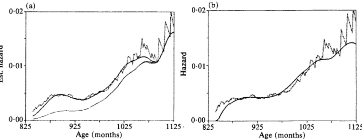
The usual identifiability assumption that aG - aw may not be reasonable here but, as mentioned earlier, this does not matter for hazard rate estimation. Due to the boundary problems and since there are only two Y's, 777 and 781, below 840 and three of them above 1125 we report only the results on the interval [840, 1125] although all the data were used in the estimation procedures. The kernels Ko and K2 are the same as in ? 5. A fixed bandwidth b = 50 is chosen for both A(z) in (2-8) and X(z) in (2.12) for all z in [840, 1125]. The results are given in Fig. 5(a). There is an increasing trend in the hazard function which is expected. This data set has also been analyzed in the past as randomly censored data only. To see how the estimates would differ had the truncation factor been ignored, the same sample is analyzed by letting the truncation variable T 0 and the resulting A(z) is displayed in Fig. 5(a) with the thinner solid line. It is clear that the hazard rate is underestimated uniformly when the truncation effect is ignored and the discrepancy is larger for smaller z's due to the left truncation scheme. This emphasizes the importance of accounting for the truncation effect. Otherwise the result can be optimistically misleading. As for the adaptive bandwidth estimators A(z, f3) with ,B in (4-6) and A(z, 83) with /3 in (3 9), initial global bandwidths bdo = 50, bd2= 100 are used for k(z) and A(2)(z) with adaptive bandwidths truncated to 70 if it exceeds 70. The resulting truncated adaptive bandwidth estimators are displayed in Fig. 5(b), where the increasing trend in hazard rate is even more visible now than in Fig. 5(a). The hazard rate increases rapidly in the early ages below 900 months, i.e. 75 years old, then stabilizes

308 ULKO UZUNOGULLARI AND JANE-LING WANG 0-02 (a) 0 02|(b) O8259512112 O825 (2b)2512 N 0*01- N 0*01- 825 925 1025 1125 825 925 1025 1125

Age (months) Age (months)

Fig. 5. (a) Estimated hazard rate for Channing House data; fixed bandwidth b = 50; darker solid line, A; thinner solid line, kwith the truncation effect neglected; dotted line, A. (b) Adaptive estimators for Channing House data; initial bandwidth bdo = 50, bd2 = 100 with adaptive bandwidths truncated above at 70; solid

line, A; dotted line, A.

between the months 900-960, i.e. ages 75-80, and starts to rise steadily again after age 80. The slight drop near 1120 months, or 93 years, is probably due to boundary effects.

ACKNOWLEDGEMENTS

Research supported in part by an U.S. Air Force Grant. The work of Ulkiu Uzunogullari was done while she was a Ph.D. student at the Department of Statistics, the Wharton School of the University of Pennsylvania. The authors would like to thank the referees for valuable suggestions.

APPENDIX

Proof of Theorem 3 2

To establish the bias and variance expression in Theorem 3 2 we need the following lemma. LEMMA A 1. We have:

(a) E{C.(z)}= C(z) + k.C'(z);

(b) var {Cn(z)}= n 1C(z)C(z)+k 2C (z){I-C (z)-2k-C(z)};

(c) E({Cn(z)-k)= 0(1), for any integer k 1; (d) E({C.(z) - _C(z)}4) = (n-2);

(e) E({C.(z) - C(z)}8) =0(n-4

Proof. Express nC6(z) = BI(B > 0) + nknI(B = _{0), where B - Binomial (n, C(z)). Parts (a) and} (b) follow from direct calculations. Part (c) follows from C(z) < 1 and

E[{Cn(z)}k < (n + I)kCn(Z)+{C(z)}-k(k+ 1)!. Note that (2s 11) implies that

E [{ Cn (z) -Cn (z)} ] = O C (z)},

for any integer k ? 1. Therefore it suffices to prove

in part (d). Notice that Cn (z) - C (z) = n1 l; 7I , where 7Bi are independent and identically dis- tributed mean zero random variables with values between 0 and 1. Therefore when taking expectation of (X m7i)4 only the terms E(iqnjq) and E(q4) are nonzero. Thus we have

E[{C.(z) - _{C(z)}4] =} n4 [nE(?i 4) + ( {E(r')} j = O(n

Part (e) follows by a similar combinatorial argument as in part (d) that

E[{C. (z) -C (z)}8] = O(n -4). C]

Proof of Theorem 3-2. Consider

X(z)-A(z) = _{*(Z)({C(Z)} -_{C(Z)}-1)} + {C(z)}-'[W*(Z(z) -] + {C(z)}-[E{i*(z)} -w_*(z)]

=1+11+111. (A 1)

By the Cauchy-Schwarz inequality, we have

Fri1 _[W*(ZVI2E [ ,, (z) C(Z) ~2

{E(I)}2 E Ew*'z)j

(zE

C

A-, M for some constant M. Applying the Cauchy-Schwarz inequality to the second term B in (A*2) we obtain, for Lemma A l(c), (d), that B=O(n-1). We have thus shown that E(I)=

O(n-112). The bias part in (3 6) now follows from (3 3) and (A 1).

Using similar arguments as above and Lemma A 1(e) with some calculations it can be shown that E(12) = O(n-1). Hence var (I) = O(n-1) = o((nb)-1). The variance part in (3 6) now follows from Lemma A 1(c) and (3 4), applying the Cauchy-Schwarz inequality to cov (I, II) and replacing

w*/C by A. n

REFERENCES

ABRAMSON, I. (1982). Arbitrariness of the pilot estimator in adaptive kernel methods. J. Mult. Anal. 12,562-7. BLUM, J. R. & SUSARLA, V. (1980). Maximal deviation theory of density and failure rate function estimates

based on censored data. In Multivariate Analysis-V, Ed. P. R. Krishnaiah, pp. 213-22. Amsterdam: North-Holland.

HYDE, J. (1977). Testing survival under right censoring and left truncation. Biometrika 64, 225-30. KRIEGER, A. M. & PICKANDS, J. III (1981). Weak convergence and efficient density estimation at a point.

Ann. Statist. 9, 1066-78.

MIULLER, H. G. (1988). Nonparametric Regression Analysis of Longitudinal Data, Lecture Notes in Statistics, 46. Berlin: Springer-Verlag.

MULLER, H. G. & WANG, J. L. (1990). Locally adaptive hazard smoothing. Prob. Theory Rel. Fields 85, 523-38. PATIL, P. N., WELLS, M. T. & MARRON, J. S. (1992). Kernel based estimation of ratio function. J. Nonpara.

Statist. To appear.

RAMLAU-HANSEN, H. (1983). Smoothing counting process intensities by means of kernel functions. Ann. Statist. 11, 452-66.

RICE, J. (1984). Boundary modification for kernel regression. Comm. Statist. A 13, 893-900.

RICE, J. & ROSENBLATT-, M. (1976). Estimation of the log survivor function and hazard function. Sankhyia A 38, 60-78.

SCHUCANY, W. R. (1989). Locally optimal window widths for kernel density estimation with large samples. Statist. Prob. Letters 7, 401-5.

STRUTHERS, C. A. & FAREWELL, V. T. (1989). A mixture model for times to AIDS data with left truncation and an uncertain origin. Biometrika 76, 814-7.

TANNER, M. A. & WONG, W. H. (1983). The estimation of the hazard function from randomly censored data by the kernel method. Ann. Statist. 11, 989-93.

310 ULKU UZUNOGULLARI AND JANE-LING WANG

TSAI, W. Y., JEWELL, N. P. & WANG, M. C. (1987). A note on the product limit estimator under right censoring and left truncation. Biometrika 74, 883-6.

WANG, M. C. (1987). Product limit estimates: A generalized maximum likelihood study. Comm. Statist. A 16, 3117-32.

WATSON, G. S. & LEADBETTER, M. R. (1964). Hazard analysis, I. Biometrika 51, 175-84.

WOODROOFE, M. (1985). Estimating a distribution function with truncated data. Ann. Statist. 13, 163-77. YANDELL, S. B. (1983). Nonparametric inference for rates with censored survival data. Ann. Statist. 11,

1119-35.