Default pricing for mortgages in Turkey

DEFAULT PRICING for MORTGAGES in TURKEY

ONUR BAŞ

105626013

ĐSTANBUL BĐLGĐ ÜNĐVERSĐTESĐ

SOSYAL BĐLĐMLER ENSTĐTÜSÜ

FĐNANSAL EKONOMĐ YÜKSEK LĐSANS PROGRAMI

YRD. DOÇ. DR. ORHAN ERDEM

2009

ii

DEFAULT PRICING for MORTGAGES in TURKEY

Onur BAŞ

105626013

Tez Danışmanı : Asst. Prof. Dr. Orhan ERDEM

...

Jüri Üyesi

: Assoc. Prof. Dr. Ege YAZGAN

...

Jüri Üyesi

: Asst. Prof. Dr. Cem DEMĐROĞLU ...

TABLE OF CONTENTS

I. INTRODUCTION. ... 1

II. THE MODEL ... 6

II.1. Assumptions ... 6

II.2. The House Price ... 6

II.3. Black-Scholes-Merton Pricing Formula ... 7

II.4. Default Rate ... 8

II.5. Risk Premium ... 10

II.6. Data Description ... 11

II.7. The Model Results ... 12

II.8. The Crisis Scenario ... 15

III. CONCLUSION ... 17

iv LIST OF FIGURES

Figure II.4.1. Default Rate (2006-2009). ... 9

Figure II.4.2. Justified Default Rate... 10

Figure II.7.1. Risk Premium, Loan to Value Ratio and House Price Variance. ... 13

Figure II.7.2. Risk Premium, Loan to Value Ratio and Conract Rate. ... 14

Figure II.8.1. Istanbul Stock Exchange and Non-Performing Consumer Loans Ratio... 15

Figure II.8.2. Risk Premium, Loan to Value Ratio and House Price Variance for Crisis Scenario. ... 16

LIST OF TABLES

Table II.6.1. The Parameters Used in The Model. ... 11 Table II.7.1. Risk Premiums for Different LTV Ratio and House Price Variance Levels. . 12 Table II.7.2. Risk Premiums for Different LTV Ratio and Contract Rate Levels. ... 14 Table II.8. Risk Premiums for Different LTV Ratio and Contract Rate Levels for Crisis Scenario. ... 16

vi ÖZET

Bu çalışma, mortgage kredilerindeki risk primini opsiyon fiyatlama tekniğine göre hesaplamayı amaçlamaktadır. Çalışmada mortgage yükümlülükleri mortgage kredisi sahiplerinin temerrüt etme ya da etmeme tercihlerine göre oluşturulan bir put opsiyonu gibi değerlendirilmiştir. Uygulama olarak da Türkiye’de ticari bir bankadan datası alınan mortgage kredisinin risk primi hesaplanmıştır.

ABSTRACT

This study tries to calculate the risk premium of a mortgage loan using an option-based pricing framework. The mortgage loan commitments are valued as put options under the consideration of mortgage holders’ choice to default or not to default. We used real mortgage data from a Turkish commercial bank, and ended up with a numeric result for the risk premium.

I. INTRODUCTION

The global financial crisis started to show its financial effects in August 2007 and emerged in Septemper 2008. Markets around the world lost value since the crisis started and governments started to play the leading role by announcing rescue packages to heal their financial systems. Actual and expected credit losses on U.S. mortgages were the main reasons for the crisis.

To begin with, mortgage loans were increasing and asset prices were appreciating till the first symptoms of the crisis appeared. During this period lending standards seemed to ease in U.S. Subsequent to this fluctuation mortgage loans became more available for risky borrowers and loan to value ratios increased. When house price appreciation ended and decline in house prices started, low-income and risky borrowers tended to default. These defaults caused mortgage-backed securities to default or to be downgraded. The market forced financial institutions to decrease the value of the securities held as assets on their books through write-downs, significantly reducing the book value of these assets to reflect the decreased market value and recording these adjustments as losses on the income statement. The financial insititutions that holds these securities in their assets had to write off these losses.

The recent economic crisis showed that mortgage loan defaults have important impacts on financial markets. The rising volume of the mortgage loans and mortgage loan default rates and their results raise the importance of pricing these assets and predicting the default behaviour of mortgage loan borrowers. For this reason option pricing method can be useful for valuation of the mortgage loans since the model has the power to project the default behavior in itself.

In U.S. lenders have been using risk-based interest rate pricing or credit scores since the mid 1990s. The premium paid per unit of risk did indeed become significantly larger over this time period (Edelberg, 2003). Lenders began to use estimates of default risk to assess different interest rates for mortgage loans because of the decrease in data storage costs and improvement in underwriting technology. Financial and demographic characteristics such as age, marriage status, number of children, whether the family has a checking account or not, education, income, net worth, level of assets, variables that reflect borrowing attitudes

and credit card expenses are the main indicators for lenders to score the risk level for a borrower. In this respect, risk-based pricing can be described as the practice of lenders charging each borrower a specific interest rate based on credit risk rather than charging one single house rate. A greater emphasis was placed on lending in lower income neighborhoods and to lower income borrowers, increasing the profitability of developing a technology to lend to higher risk households. Adding to the pressures on conventional lenders, Fannie Mae – which previously had purchased only low-risk loans and essentially did not vary any of the financial terms with the riskiness of the loan – introduced a new and improved automated underwriting system in 1995 and began to accept higher risk loans (Edelberg, 2003). Subsequently, Fannie Mae began to change some of the terms with the loan’s level of risk. In 1996 both Fannie Mae and Freddie Mac made it clear that lenders who wanted to sell mortgage loans (to them) would be well-advised to include a credit bureau score as part of the loan package (McCorkell, 2002). Accordingly, lenders could, and did, begin to issue higher risk mortgages (Freeman and Hamilton, 2002). The results of this pricing system is the premium paid per unit of risk increased over this time period with the difference between high- and low-risk borrowers’ interest rates at least nearly doubling for mortgage loans (Edelberg, 2003). There are many arguments if interest rates and fees paid by mortgage borrowers reflect the cost and risk in risk-based pricing system.

In Turkey mortgage pricing includes default risk but there is not a sophisticated risk-based scoring system like it is in U.S. Funding cost, net income from the loan and default cost are the main indicators for pricing. Default risk is taken into account according to the historical default performance of the borrowers. In order to be compatible with Basel II standards Turkish banking system is developing its structure for risk-based scoring system but the system has not been started to be implemented exactly.

Various mortgage derivative pricing techniques are available in the literature. Option-based pricing techniques are one of those. The idea which comes from modeling mortgage derivatives as options goes back to Merton (1977), who derives a formula to evaluate the price of the loan insurance. The seminal contributions of Black and Scholes (1973), and Merton (1973) are among the other most influential papers in option pricing. Option pricing methologies can be divided into two sub catagories: Models with strategic prepayment and default characteristic, models with exogenous prepayment and default

3

characteristic. Kau et al (1985), Kau et al (1993), Crawford and Rosenblatt (1995), Kau and Slawson (2000), Hilliard et al. (1998) are of the first type. Kalotay et al (2004) supports these type of models with empirical evidence. Bardhan et al (2006) is of the second type. They question the strategic prepayment and default in the sense that not all the people act as if they are financial engineers. As a result they take the loss of the insurer as an option, and using Black and Schole’s formula come up with a closed form formula for the mortgage insurance premium that the borrower is supposed to pay. Their findings are in line with Hendershott and Van Order (1987).

Kau et al (1993) used option pricing techniques for determining the effect of changes in mortgage contracts or in the economic environment. According to their model the prepayment decision is influenced by interest rates, whereas the house price influences the decision to default. Default occurs when the value of the mortgage to the lender, which is the cost of the mortgage to the borrower, exceeds the house price. Default does not occur as soon as the value of promised payments exceeds the value of the house, because this would ignore the value of being able to terminate the contract in the future. Thus the house price and the term structure of interest rates were chosen as the underlying sources of uncertainty in the model. The value of the house was assumed to follow a standard lognormal process. The results indicate that considerable variability in insurance prices is required in order to respond to changes in loan to value ratios and house prices and their study revealed that option pricing models can be useful for mortgage insurance pricing. Crawford and Rosenblatt (1995) showed theoretically and empirically the effect of frictions on the individual strike price by option pricing method. When transaction costs are considered, the rational borrower will default only when the value of the collateral falls below the mortgage value by an amount equal to the net transaction costs. The transaction costs which they included were the costs of moving, brokerage fees, taxes, future deficiency payments, and the stigma associated with default; and are offset by free rents during delinquency. Since, for most borrowers, net transaction costs are positive, Standard measures of equity may be significantly negative by the time the rational borrower exercises the default option (Crawford & Rosenblatt, 1995). Their study indicated that transaction costs influence a borrower’s strike price and reduce the probability of default. Kau and Slawson (2000) extended option pricing method by adding transaction costs, suboptimal termination and decision probabilities. The purpose of their study was to

consolidate previous works that depart from the frictionless model. They developed a model for pricing a mortgage which allows for transaction costs for both default and prepayment, suboptimal termination together with separate transaction costs for default and prepayment, and suboptimal nontermination through the use of decision probabilities. Since it can handle transaction costs, bivariate binomial model was used in a contingent claims framework. Transaction costs are prepayment penalties whereas suboptimal termination occurs when the borrower terminates the mortgage by either prepaying or defaulting for exogenous (nonfinancial) reasons, such as divorce and a job in another state. Decision probabilities are explanation for suboptimal non-termination when the financial model says that the borrower should. The model allowed the borrower to make specific decisions at each point in time and, because of this, the binomial model is easily extended to include frictions. The pricing of a mortgage involved the modeling of the underlying state variables. The state variables used in the study were house price and the spot rate of interest. The standard lognormal process was used for the house price. The results showed that any increase in transaction costs, increases the value of the mortgage asset for both the lender and the borrower.

Differently from the methods mentioned above, Bardhan et al (2006) used an option pricing method developed by Black and Scholes and Merton (1973) for valuing the mortgage insurance contracts. They calculated the risk premium according to the borrower’s default by representing the default as a portfolio of put options on the borrower’s collateral. They assumed that agents in the economy are risk neutral. In their model collateral value is assumed as a risk-free asset in the economy and has a constant return followed a geometric Brownian motion process. They also quantified the legal inefficiencies and took them into account when pricing mortgage insurance contracts. In contrast to related litareture, there is only one state variable in the model namely the collateral value. The interest rate was not included to the model as a state variable that is consistent with the empirical findings reported in Hendershott and Van Order (1987) who provide evidence that mortgage insurance premiums are not very sensitive to interest rate volatility. Their study indicated that mortgage insurance premium increases, ceteris paribus, with an increase in volatility of the collateral, the probability of default, the mortgage contract rate (or, equivalently, mortgage installment payments), or the time delay in the repossession of the collateral. As they priced a Serbian government-backed mortgage insurance contracts their study marked that their method can be useful in

5

emerging market economies where other methods may be difficult or complex to implement.

In this study option pricing theory which is developed by Bardhan et al is used for the valuation of mortgage loans. There are two main reasons why I apply this method. Firstly, it is simple to use. Secondly, it is based on real data. For the risk premium calculation, smoothed actual default rates of TL mortgage loans have been used in the model. The mortgage loan commitments are valued as put options under the consideration of mortgage holders choice to default or not to default till the expiration date of the mortgage liability. The house price is assumed to follow a stochastic process in the model, for this reason, the house price is calculated according to the Geometric Brownian motion. The difference between the house price and remaining loan balance is described as the borrower’s portfolio and the main assumption is that the borrowers act to maximize this portfolio. Set of default choices till the expiration date of the mortgage loan determines the risk premium for the lender and the risk premium is equal to the sum of the present values of the every month’s expected loss. Default choice probabilities are calculated exogenously out of the model and included to estimate the expected loss for each option decision. In the study actual default rates of TL mortgage loans of a commercial bank have been used.

In order to analyse the properties of the model, different sets of numerical solutions were examined. Since it is assumed that the house price follows a random walk, average of many numerical calculations are taken as the model results in order to avoid possible abnormalities in the study.

The study proceeds as follows. In the next section, the model is defined. Firstly, assumptions of the model are summarized and option pricing formula used in the study is presented. Then, default rate is described in detail and risk premium calculation is expressed. Next, data and methodology are presented. Finally, results for different economic parameters are revealed and analysed. In the conclusion, our findings and ideas are summarized.

II. THE MODEL II.1. Assumptions

In our model there are two sides in the economy: the lender and the borrower. The lender gives T-year mortgage loan (B0) to the borrower for the amount of loan to value ratio

(LTV) times the collateral value which is house price in our study (H0) at t=0. The mortgage loan has a fixed interest rate (c) till the expiring date and is supposed to be higher than risk free interest rate (r).

At time t = 0; B0 = LTV*H0

0 ≤ t ≤ T c > r

c and r are the monthly interest rates and it is assumed that loan payments are paid monthly. Then we can write the monthly payment amount (y);

T 0 0

y = B c B c(1 c)− + II.2. The House Price

The house price (H) is assumed to follow a standard log-normal process as Black and Scholes and Merton developed in 1973.

Any variable whose value changes over time in an uncertain way is said to follow a stochastic process (Hull, 2003). Historical values of a variable have not got an effect on the present value and the future value of the variable. Only the present value of the variable has the power to predict the future value. Predictions for the future are uncertain and must be expressed in terms of probability distributions (Hull, 2003). The process followed by the house price in the model is a Wiener process.

The house price (H) is assumed to follow a standard Geometric Brownian Motion:

H H

dH(t)

( s)dt dz

7

This formula represents the Geometric Brownian motion in which dzH is a Wiener process.

µ is the expected return on the house (collateral) and s is the service flow. We assume s as a dividend in Black, Scholes and Merton (1973). In the absence of the taxes service flow s is the rent house should earn (Kau, 1993) and it is represented as the percentage of the house price. σH is the standard deviation of the house price. (µ-s)dt term indicates that

house price (H) has an expected drift rate of risk free rate minus service flow rate (µ-s) per unit of time. (µ-s) can be described as the expected growth rate of the house price. σH dzH

term adds variability to the path followed by the house price (H). After applying the model Black, Scholes and Merton developed, it is assumed that percentage changes in house price in a short time period are normally distributed.

As a result change in house price depends on the current house price and unpredictable component. Since we assume that agents in the economy are risk neutral, expected return on collateral is equal to the risk free interest rate (µ = r) (Kau, 1998). Because the risk neutral investors do not require risk premium, all expected returns on all assets become equal to the risk free rate. This assumption will also provide to discount expected payoffs at the risk free interest rate.

II.3. Black-Scholes-Merton Pricing Formula

The mortgage loan is a put option that allows the borrower to sell the value of his indebtedness in return for the proceeds from the loan (Kutner, 1989).

Black, Scholes and Merton option pricing theory with constant dividend yield is used in our model for the valuation of the mortgage loan. In the option pricing theory strike price is the remaining loan balance.

(

)

(

)

p is price of the European put option and s is the rent income of the house. r is the risk free interest rate and H0 is the house price at time zero. K is the strike price and it represents the

remaining loan balance in the model where σ stands for house price volatility. In the formula N(x) is the cumulative probability distribution function for a standardized normal distribution.

Option pricing theory reflects the mortgage holders behaviour. When the cost of the mortgage to the borrower exceeds the house price, the default occurs. The difference between the house price and remaining loan balance can be described as the borrower’s portfolio. The borrower takes decisions in order to maximize this portfolio. The borrower has two alternatives to maximize his position which can be achieved either by defaulting or continuing his loan. Borrower’s decision to default or not to default depends on the remaining loan balance and the house price. If the house price (Ht) is greater than the

remaining mortgage loan balance, there is no need for borrower to pay the loan balance and defaults, but if the remainig mortgage loan balance is less than the house price, the borrower does not default.

II.4. Default Rate

In the model the mortgage risk premium is equal to the sum of the present values of the every month’s expected loss. Expected loss for a month during the mortgage life is equal to the weighted put option value by the conditional probability of default at that month. The conditional probability of defaulting at time t is equal to the probability of not to default at time (t-1) times probability of default at time t.

9

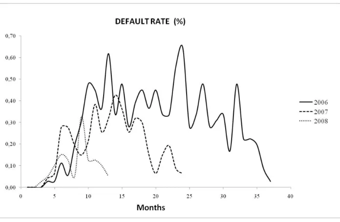
Figure II.4.1. Default Rate (2006-2009)

Figure II.4.1. shows the actual default rates of TL mortgage loans of a commercial bank between 01.01.2006 and 31.01.2009. The graph represents the what percentage of the TL mortgage loans defaulted at which month since the beginning of the loans.

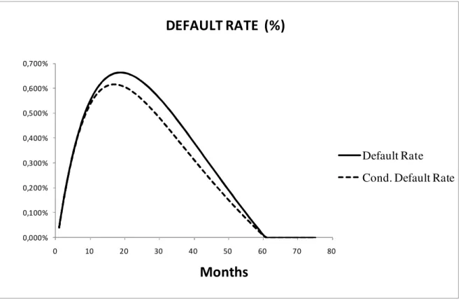
Figure II.4.2. Justified Default Rate 0,000% 0,100% 0,200% 0,300% 0,400% 0,500% 0,600% 0,700% 0 10 20 30 40 50 60 70 80 Default Rate Cond. Default Rate

DEFAULT RATE (%)

Months

Figure II.4.2. is the exponentionally smoothed version of the Figure II.4.2.

II.5. Risk Premium

Default decision is mathematically represented by the put option computation in option pricing theory. There are t put options in number till the expiration date and sum of conditional default rate weighted put option values give the mortgage risk premium. Upon stating Black-Scholes-Merton pricing formula and the conditional default rate, present value of the risk premium (RP0) is given by the following expression:

( )

∑

Pd(t): Conditional probability of defaulting at time t

p(t): Put option value at time t r: Risk free interest rate

RP0 can be defined as the present value of the accumulated expected loss of a mortgage

11 II.6. Data Description

The mortgage loan is a put option that allows the borrower to sell his indebtness in returns for the proceeds from the loan. The most important component of this commitment is the house price. The borrower can exercise the option depending upon the changes in house price between the time the commitment is made and the time at which the commitment expires.

In the study actual default rates of TL mortgage loans of a commercial bank between 01.01.2006 and 31.01.2009 have been used (The name of the bank is not revealed for confidental purposes). This data is used to calculate the conditional and unconditional default rate. After building the data set each month’s average default rate has been calculated but this data has not been used directly in numerical analysis. In order to forecast the default rate of the following months after 31.01.2009, the data has been justified by the sample-fit model which was developed by Nelson and Siegel in 1987.

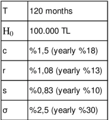
Table II.6.1. The Parameters Used in The Model T 120 months H0 100.000 TL c %1,5 (yearly %18) r %1,08 (yearly %13) s %0,83 (yearly %10) σ %2,5 (yearly %30)

The put option value is linear in the size of the loan and depends on the risk free interest rate, contract rate, maturity, loan to value ratio (LTV), house price volatility and rent return. The numerical solutions have been provided to analyze the effect of house price volatility, LTV ratio and the contract rate. In the analysis it is also assumed that there are no transaction costs but related literature revealed that transaction costs increase the option value.

II.7. The Model Results

In order to analyse the properties of the model, different sets of numerical solutions were examined. Since it is assumed that house price follows a random walk, every result is the average of many numerical calculations.

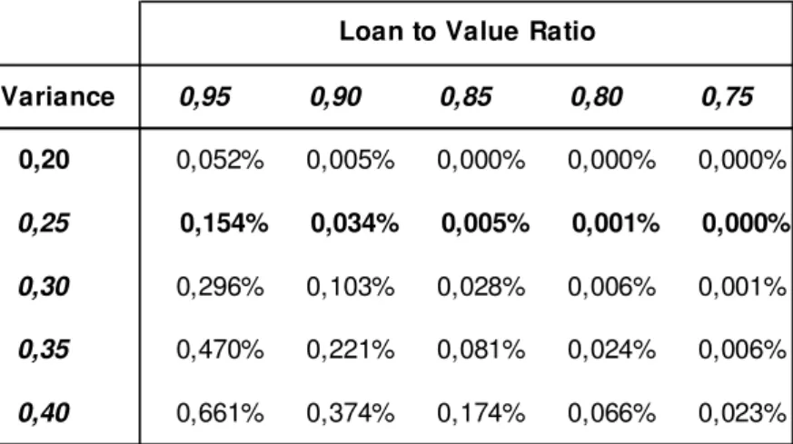
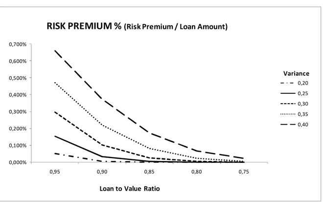
The effects of house price variance and LTV ratio are shown in Table II.7.1. The risk premiums are represented as a percentage of mortgage loan since absolute risk premium values can be meaningless as the mortgage loan balance changes according to the LTV ratio changes. The results are compatible with the expectations.

Table II.7.1. Risk Premiums for Different LTV Ratio and House Price Variance Levels

Variance 0,95 0,90 0,85 0,80 0,75 0,20 0,052% 0,005% 0,000% 0,000% 0,000% 0,25 0,154% 0,034% 0,005% 0,001% 0,000% 0,30 0,296% 0,103% 0,028% 0,006% 0,001% 0,35 0,470% 0,221% 0,081% 0,024% 0,006% 0,40 0,661% 0,374% 0,174% 0,066% 0,023%

Loan to Value Ratio

The most significant parameter is the LTV ratio. LTV ratio determines the loan amount and the promising payments of the borrower. Our calculations confirm that increase in LTV ratio makes the risk premium greater.

There are different calculation results for several house price volatilities in Table II.7.1. Effect of increased house price volatility raises the risk premium which is consistent with the theoretical predictions.

Graphical representation of the results is displayed in Figure II.7.1 and shows that the change in house level variance shifts the risk premium curve. While increase in variance level shifts the risk premium curve to the right, decrease in variance shifts the risk premium curve to the left. The house price variance is assumed to be 25% in Turkey. The results under different volatility possibilities for the future are also simulated.

At low levels of LTV ratio risk premium calculation can be ignored since it is about 0,001% at 80% LTV ratio, but as it gets higher, risk premium becomes significant and

13

should be included in pricing. There is no any legal pressure for LTV ratio in Turkey, but banks generally tend to give mortgage loans at 75-80% of the house price for risk aversion. Although low LTV mortgage loans are dominating the mortgage loan composition in Turkey, mortgage loans over 80% LTV ratio can not be underestimated. If risk perception changes and high LTV ratio mortgage loans’ weight starts to increase, option pricing technique can be essential.

Figure II.7.1. Risk Premium, Loan to Value Ratio and House Price Variance

0,000% 0,100% 0,200% 0,300% 0,400% 0,500% 0,600% 0,700% 0,95 0,90 0,85 0,80 0,75 0,20 0,25 0,30 0,35 0,40

RISK PREMIUM %

Loan to Value Ratio

Variance

As can be seen from the figure above change in LTV levels causes changes along the risk premium curve. Increase in LTV raises risk premium values while the decrease in LTV ratio reduces the risk premium.

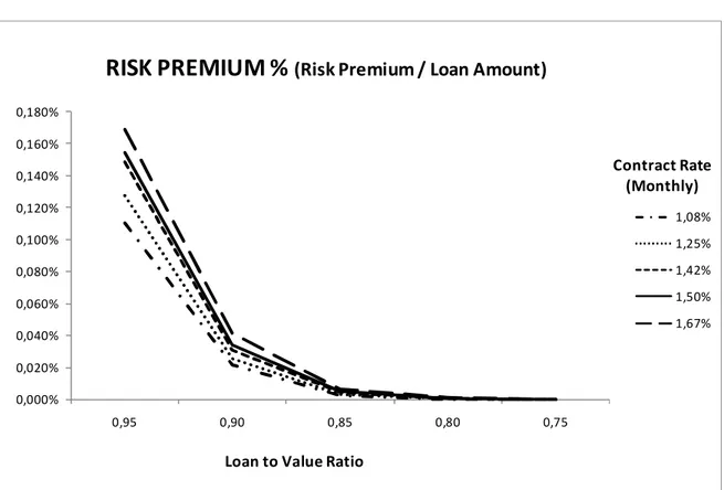
Table II.7.2 shows the different risk premiums for different contract rates. It is obvious that risk premium increases as the contract rate increases. Like LTV ratio, contract rate affects option value and has a positive relation with risk premium. As contract rate increases, mortgage liability of the borrower increases, too. However the effect of contract rate is more limited than the LTV ratio and house price variance.

Table II.7.2. Risk Premiums for Different LTV Ratio and Contract Rate Levels

Conract Rate (Monthly) 0,95 0,90 0,85 0,80 0,75

1,08% 0,110% 0,022% 0,002% 0,000% 0,000%

1,25% 0,127% 0,026% 0,004% 0,000% 0,000%

1,42% 0,149% 0,031% 0,005% 0,001% 0,000%

1,50% 0,154% 0,034% 0,005% 0,001% 0,000%

1,67% 0,169% 0,041% 0,007% 0,001% 0,000%

Loan to Value Ratio

Figure II.7.2 shows different combination of opportunity costs.

Figure II.7.2. Risk Premium, Loan to Value Ratio and Conract Rate

0,000% 0,020% 0,040% 0,060% 0,080% 0,100% 0,120% 0,140% 0,160% 0,180% 0,95 0,90 0,85 0,80 0,75 1,08% 1,25% 1,42% 1,50% 1,67%

RISK PREMIUM %

Loan to Value Ratio

Contract Rate (Monthly)

15 II.8. The Crisis Scenario

Figure II.8.1. Istanbul Stock Exchange and Non-Performing Consumer Loans Ratio

Ja n u a ry 0 6 M a rc h 0 6 M a y 0 6 Ju ly 0 6 S e p te m b e r 0 6 N o v e m b e r 0 6 Ja n u a ry 0 7 M a rc h 0 7 M a y 0 7 Ju ly 0 7 S e p te m b e r 0 7 N o v e m b e r 0 7 Ja n u a ry 0 8 M a rc h 0 8 M a y 0 8 Ju ly 0 8 S e p te m b e r 0 8 N o v e m b e r 0 8 Ja n u a ry 0 9 ISTANBUL STOCK EXCHANGE INDEX NON-PERFORMING CONSUMER LOANS RATIO

ISTANBUL STOCK EXCHANGE INDEX &

NON-PERFORMING CONSUMER LOANS RATIO

Stock exchange index is an important indicator for the economic performance. Figure II.8.1 shows that non-performing consumer loans ratio increases during the period where Istanbul Stock Exchange decreases. Because non-performing mortgage loans data do not exist for Turkish banking sector, total consumer loans (mortgage, auto and general purpose loans) performance is used in Figure II.8.1.

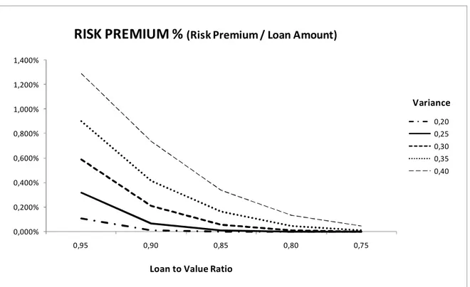
When the economy collapses, it is expected that consumer loans default rate and house price variance increase. Table II.8. shows risk premiums for different variance levels and LTV ratios if the default rate doubles.

Table II.8. Risk Premiums for Different LTV Ratio and Contract Rate Levels for Crisis Scenario Variance 0,95 0,90 0,85 0,80 0,75 0,20 0,110% 0,011% 0,001% 0,000% 0,000% 0,25 0,317% 0,069% 0,011% 0,001% 0,000% 0,30 0,586% 0,211% 0,057% 0,011% 0,002% 0,35 0,899% 0,413% 0,168% 0,050% 0,013% 0,40 1,291% 0,738% 0,335% 0,133% 0,045%

Loan to Value Ratio

Figure II.8.2. Risk Premium, Loan to Value Ratio and House Price Variance for Crisis Scenario 0,000% 0,200% 0,400% 0,600% 0,800% 1,000% 1,200% 1,400% 0,95 0,90 0,85 0,80 0,75 0,20 0,25 0,30 0,35 0,40

RISK PREMIUM %

Loan to Value Ratio

17 III. CONCLUSION

In this study option pricing theory is used for the valuation of mortgage loans. Mortgage holders behaviour is reflected by the option pricing theory.

The model results marked that the findings are compatible with the predictions and similar with the related literature. Firstly, LTV ratio and house price variance are the main parameters that affect mortgage loan risk premium. Both of them have got significant effects on the magnitude of the risk premium. In addition, contract rate has also effect on risk premium. Like LTV ratio, contract rate affects option value and has a positive relation with risk premium. As contract rate increases, mortgage liability of the borrower increases, too. However, results indicate that the effect of contract rate is more limited than LTV ratio and house price variance.

At low levels of LTV ratio risk premium calculation can be ignored since it is about 0,001% of the mortgage loan at %80 LTV ratio but as it gets higher risk premium becomes significant and should be included in pricing. There is no any legal pressure for LTV ratio in Turkey, but banks generally tend to give mortgage loans at 75-80% of the house price for risk aversion. Although low LTV mortgage loans are dominating the mortgage loan composition in Turkey, mortgage loans over 75% LTV ratio can not be underestimated. If risk perception changes and high LTV ratio mortgage loans’ weight starts to increase, option pricing technique can be essential.

Considering the findings of the present study, several suggestions for further research can be made. Prepayment decisions and transaction costs can be included in the model so that their effect on risk premium can also be analyzed.

REFERENCES

Ambrose, B.W. & Buttimer, R.J. & Capone, C.A. (1997). Pricing mortgage default and foreclosure delay. Journal of Money, Credit and Banking, 29(3), 314-325.

Banking Regulation and Supervision Agency Statistical Data. Retrieved July 1, 2009 http://www.bddk.org.tr/websitesi/turkce/Istatistiki_Veriler/Istatistiki_Veriler.aspx

Bardhan, A. & Karapandza, R. & Urosevic, B. (2006). Valuing mortgage insurance contracts in emerging markets. The Journal of Real Estate Finance and Economics, 32(1), 9-20.

Black, F. & Scholes, M. (1973). The Pricing of Options and Corporate Liabilities. Journal of Political Economy, 81, 637-654

Brealey, R.A. & Myers, S.C. & Allen, F. (2006). Corporate Finance. New York: McGraw-Hill.

Clauretie, T.M. & Jameson, M. (1990). Interest rates and the foreclosure process: an agency problem in fha mortgage insurance. The Journal of Risk and Insurance, 57(4), 701-711.

Crawford, G.W. & Rosenblatt, E. (1995). Efficient mortgage default option exercise: evidence from loss severity. The Journal of Real Estate Research, 10(5), 543-555.

Edelberg, W. (2003). Risk-based pricing of interest rates in household loan markets. FEDS Working Paper, 62.

Freeman, L. & Hamilton, D. (2002). A Dream Deferred or Realized: The Impact of Public Policy on Fostering Black Homeownership in New York City Throughout the 1990's. AEA Proceedings, 92(2), 320-324.

Hendershott, P. & Van Order, R. (1987). Pricing Mortgages: Interpretation of the Models and Results. Journal of Financial Services Research 1(1), 19-55.

Hilliard, J.E. & Kau, J.B. & Slawson V.C. (1998). Valuing prepayment and default in a fixed-rate mortgage: a bivariate binomial options pricing technique. Real Estate Economics, 26(3), 431-468.

19

Istanbul Stock Exchange Closing Values of Main Stock Market Price Indices. Retrieved July 1, 2009 from http://www.ise.org/data.htm

Kalotay, A. & Yang, D. & Fabozzi, F. (2004). An Option-Theoretic Prepayment Model for Mortgages and Mortgage-Backed Securities. International Journal of Theoretical and Applied Finance, 7(8), 949-978.

Kau, J.B. & Keenan, D.C. (1999). Patterns of rational default. Regional Science and Urban Economics, 29(6), 765-785.

Kau, J.B. & Keenan, D.C. & Muller, W.J. (1985). Rational Pricing of Adjustable Rate Mortgages. Real Estate Economics, 13(2), 117-128.

Kau, J.B. & Keenan, D.C. & Muller W.J. (1993). An option-based pricing model of private mortgage insurance. The Journal of Risk and Insurance, 60(2), 288-299.

Kau, J.B. & Slawson V.C. (2000). Frictions and mortgage options. Retrieved April 14, 2009 from http://ssrn.com/abstract=191948

Kutner, G.W. & Seifert, J.A. (1989). The valuation of mortgage loan commitments using option pricing estimates. The Journal of Real Estate Research, 4(2), 13-20.

McCorkell, Peter L. (2002). The Impact of Credit Scoring and Automated Underwriting on Credit Availability. The Impact of Public Policy on Consumer Credit, eds. Thomas Durkin and Michael Staten, Massachusetts: Kluwer Academic Publishers, 209-219.

Merton, R. (1973). Theory of Rational Option Pricing. Bell Journal of Economics and Management Science, 4, 141-183.

Merton, R. (1977). An Analytic Derivation of the Cost of Deposit Insurance and Loan Guarantees: An Application of Modern Option Pricing Theory. Journal of Banking and Finance 1, 3-11.

Pooter, M. (2007). Examining the Nelson-Siegel class of term structure models in-sample fit versus out-of-sample forecasting performance. Tinbergen Institute Discussion Paper. White A.M. (2004). Risk-based mortgage pricing: present and future research. Housing Policiy Debate, 15(3), 503-531.