Investigation the risk of autism by evaluating prenatal and postnatal exposure to traffic-related air pollution

(1)

KADİR HAS UNIVERSITY SCHOOL OF GRADUATE STUDIES PROGRAM OF COMPUTER ENGINEERING

INVESTIGATION THE RISK OF AUTISM BY

EVALUATING PRENATAL AND POSTNATAL

EXPOSURE TO TRAFFIC-RELATED AIR POLLUTION

TAMER DEMİR

MASTER’S THESIS

(2)

Ta mer DEMİ R M.S . The sis 2020 S tudent’ s F ull Na me P h.D. (or M.S . or M.A .) The sis 20 11

(3)

INVESTIGATION THE RISK OF AUTISM BY

EVALUATING PRENATAL AND POSTNATAL

EXPOSURE TO TRAFFIC-RELATED AIR POLLUTION

TAMER DEMİR

MASTER’S THESIS

Submitted to the School of Graduate Studies of Kadir Has University in partial fulfillment of the requirements for the degree of Master’s in the Program of

Computer Engineering

(4)

DECLARATION OF RESEARCH ETHICS / METHODS OF DISSEMINATION

I, TAMER DEMİR, hereby declare that;

 this Master’s Thesis is my own original work and that due references have been appropriately provided on all supporting literature and resources;

 this Master’s Thesis contains no material that has been submitted or accepted for a degree or diploma in any other educational institution;

 I have followed “Kadir Has University Academic Ethics Principles” prepared in accordance with the “The Council of Higher Education’s Ethical Conduct Principles”

In addition, I understand that any false claim in respect of this work will result in disciplinary action in accordance with University regulations.

Furthermore, both printed and electronic copies of my work will be kept in Kadir Has Information Center under the following condition as indicated below:

� The full content of my thesis/project will be accessible from everywhere by all means.

TAMER DEMİR 24/06/2020

(5)

KADIR HAS UNIVERSITY SCHOOL OF GRADUATE STUDIES

ACCEPTANCE AND APPROVAL

This work entitled INVESTIGATION THE RISK OF AUTISM BY

EVALUATING PRENATAL AND POSTNATAL EXPOSURE TO TRAFFIC-RELATED AIR POLLUTION prepared by TAMER DEMİR has been judged to be

successful at the defense exam held on 24/06/2020 and accepted by our jury as TYPE

OF THE THESIS.

APPROVED BY:

Assoc. Prof. Dr. Tamer DAĞ (Advisor) Kadir Has University ______________

Assoc. Prof. Dr. Habib ŞENOL Kadir Has University ______________

Assoc. Prof. Dr. Tansal GÜÇLÜOĞLU Yıldız Technical University ______________

I certify that the above signatures belong to the faculty members named above.

_______________ Prof. Dr. Sinem AKGÜL AÇIKMEŞE Dean of School of Graduate Studies DATE OF APPROVAL: 24/06/2020

(6)

ABSTRACT

Autism spectrum disorder (ASD ) which is a group of neurodevelopmental disorder that appears during the first few years of a child’s life affecting a child’s communication and socialization abilities with increasing prevalence. Recently, several recent studies have found associations between exposure to traffic-related air pollution (TRAP) and ASD. The primary aim of this study is to investigate/examine the relation between TRAP and four air pollutants (NO2, O3, PM10, PM2.5) and ASD during prenatal or post-natal by

using multiple logistic regression models and variable selection methods. Results show that the adjusted odds ratio (AOR) for ASD per IQR increase was strongly associated for exposure to NO2 during the first year period, was moderately associated for

exposure to NO2 (from interstate highways during the third trimester; from the county

highway during the first year; from city street during the first year; from all roads during the all pregnancy; from all roads during the first trimester) and O3 during the second

year, and weakly associated with exposure to NO2 from interstate highways during the

second trimester, O3 during the first trimester and PM2.5 during the second year.

Additionally, comparing fourth to first quartile exposures the AOR was 15.47 for NO2

from interstate highways during the third trimester, was 5.00 for NO2 from all roads

during the first trimester, and comparing third to first quartile exposures the AOR was 2.31 for PM2.5 during the second year. As a result, a strong relationship between NO2

exposure and ASD was detected for each 7.1 ppb [IQR] increase in NO2 during the first

year and subjects exposed to a higher level of NO2 during the first and third trimester,

and PM2.5 during the second year was also associated with increased risk of ASD.

Keywords: Autism spectrum disorder (ASD), Air pollution, Multiple logistic

(11)

ii

DOĞUM ÖNCESİ VE SONRASI TRAFİK KAYNAKLI HAVA KİRLİLİĞİNE MARUZ KALMA İLE OTİZM SPEKTRUM BOZUKLUĞU (ASD) ARASINDAKİ

İLİŞKİYİ ORTAYA ÇIKARMAK

ÖZET

Otizm spektrum bozukluğu (ASD), hızlıca artan bir yaygınlıkla çocukluğun ilk yıllarında ortaya çıkan ve çocuğun iletişim ve sosyalleşme yetilerini etkileyen nörogelişimsel bozuklular grubudur. Son zamanlarda trafik kaynaklı hava kirliliğine (TRAP) maruz kalma ve Otizm spektrum bozukluğu (ASD) arasındaki ilişkiyi ortaya çıkaran çalışmalar yapılmıştır. Bu çalışmanın temel amacı, trafik kaynaklı hava kirliliği ve 4 hava kirleticisi (NO2, O3, PM10, PM2.5) ve Otizm spektrum bozukluğu (ASD)

arasındaki ilişkiyi lojistik regresyon modellerini ve değişken seçim yöntemlerini kullanarak ortaya çıkarmak / incelemektir. Sonuçlar, [IQR] artışı başına ASD için ayarlanmış olasılık oranının (AOR), ilk yıl boyunca NO2'ye maruz kalmayla güçlü,

ikinci yıl boyunca O3’e, NO2'ye (üçüncü üç aylık dönemde eyaletler arası otoyollardan;

ilk yıl boyunca ilçe otoyolundan; ilk yıl boyunca şehir caddesinden; tüm gebelik boyunca tüm yollardan; ilk üç aylık dönemde tüm yollardan çıkan) maruz kalmayla orta derecede, ve ikinci üç aylık dönemde eyaletler arası otoyollardan çıkan NO2'ye ilk

üç aylık dönemde O3’e ve ikinci yılda PM2.5’e maruz kalma ile zayıf bir şekilde ilişkili

olduğunu göstermektedir. Ek olarak, dördüncü ve birinci çeyrek maruz kalmaları karşılaştırıldığında, üçüncü üç aylık dönemde eyaletler arası otoyollardan çıkan NO2

için AOR 15.47, ilk üç aylık dönemde tüm yollardan çıkan NO2 için 5.00 idi ve üçüncü

ile birinci çeyrek maruz kalmaları karşılaştırıldığında, AOR ikinci yılda PM2.5 için 2.31

idi. Sonuç olarak, ilk yıl NO2'deki her 7.1 ppb [IQR] artış için NO2’ye maruz kalma ile

ASD arasında güçlü bir ilişki tespit edildi ve ayrıca birinci ve üçüncü üç aylık dönem boyunca NO2’nin, ikinci yıl boyunca PM2,5’nin daha yüksek düzeyine maruz kalan

denekler artan ASD riski ile ilişkilendirildi.

Anahtar Sözcükler: Otizm spektrum bozukluğu (ASD), Hava kirliliği, Çoklu lojistik

(12)

iii

ACKNOWLEDGEMENTS

I would like to express my appreciation to all people who gave a contribution to my thesis. First and foremost, I would like to thank Assoc. Prof. Dr. Tamer Dağ for his support and guidance throughout the thesis process.

I would also like to thank my mum and my wife, Hilal, for the support they provided me throughout my entire life.

(13)

iv

DEDICATION

(14)

v

LIST OF TABLES

Table 2.1: Prevalence of ASD in 8-year-olds (2014) [18]. ... 7

Table 2.2: Prevalence of ASD based on ADDM Network studies published from 2007 to 2018 (surveillance years 2000-2014) [19]. ... 8

Table 3.1: Distance to Freeway and Major Road Data Collection ... 16

Table 3.2: “Traffic-Related Air Pollution (TRAP) Estimates” Table Attributes ... 19

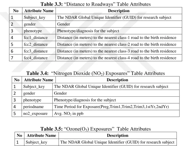
Table 3.3: “Distance to Roadways” Table Attributes ... 19

Table 3.4: “Nitrogen Dioxide (NO2) Exposures” Table Attributes ... 19

Table 3.5: “Ozone(O3) Exposures” Table Attributes ... 19

Table 3.6: “Particulate Matter 10 (PM10) Exposures” Table Attributes ... 20

Table 3.7: “Particulate Matter 2.5 (PM2.5) Exposures” Table Attributes ... 20

Table 3.8: Transformed “Nitrogen Dioxide (NO2) Exposures” Table tempNO2 ... 20

Table 3.9: Transformed “Ozone(O3) Exposures” Dataset tempO3... 21

Table 3.10: “Exposure” Dataset Attributes ... 22

Table 3.11: The distribution of the subjects in “Exposure” Dataset ... 23

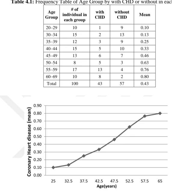
Table 4.1: Frequency Table of Age Group by with CHD or without in each group ... 33

Table 4.2 Probability( ) -Odds Relation ... 41

Table 4.3: Wald test output ... 46

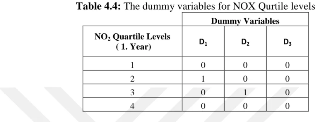
Table 4.4: The dummy variables for NOX Qurtile levels ... 56

Table 4.5: The Log-odds of Disease and Odds of Disease for Quartile levels ... 56

Table 5.1: The summary of “Exposure” table based on phenotype ... 67

Table 5.2: The summary of “Exposure” table based on gender ... 68

Table 5.3: The summary of “Exposure” table based on Autistic ... 68

Table 5.4: Statistical measures for “NdarExposure.txt” ... 69

Table 6.1: Summary results of the fitting model.full ... 77

Table 6.2: Odds ratios(OR) and confidence intervals(CI) results for each coefficient of the model.full ... 80

Table 6.3: Results of fitting of the model.full ... 83

Table 6.4: The list of selected variables that are significant at the 0.25 level... 85

(15)

vi

Table 6.6: Results of fitting of model.2 ... 87

Table 6.7: Results of fitting of model.int, the interactions whose p-values < 0.001 ... 90

Table 6.8: The results of Backward elimination w.r.t. p-value ... 95

Table 6.9: The output of the step() function with trace=1 option ... 96

Table 6.10: The output of model.s$anova ... 97

Table 6.11: Output of summary(model.s) ... 98

Table 6.12: Summary results of the fitting model.q ... 101

Table 6.13: Summary results of fitting model.q.s ... 104

Table 6.14: The OR values and their CI for model.s... 106

Table 6.15: Estimated ORs for per IQR change... 107

Table 6.16: Strength of associations with Autism... 108

Table 6.17: The OR% groups for a per IQR change ... 108

Table 6.18: The OR values and their CI for model.q.s... 109

Table 7.1: The significant or important variables w.r.t. Wald test ... 113

Table 7.2: The variables associated with ASD risk ... 114

Table 7.3 The ORs for each change in IQR for model.s ... 115

Table 7.4: The OR values > 1, the relative increase in the odds of ASD from one level of quartile to another, for model.q.s ... 116

(16)

vii

LIST OF FIGURES

Figure 1.1: Cross-Industry Standard Process for Data Mining (CRISP-DM) [13] ... 4

Figure 2.1: The Estimated ASD Prevalence Rate (per 1000) based on Table 2.2 Data .. 8

Figure 4.1: The objects in region R are outliers. ... 28

Figure 4.2: Boxplot ... 29

Figure 4.3: Mean, median, and mode of symmetric versus positively and negatively skewed data. ... 30

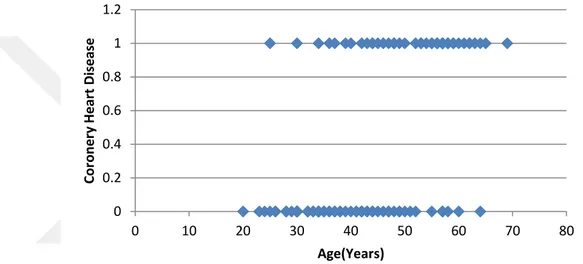
Figure 4.4: Scatterplot of coronary heart disease (CHD) status by age for 100 subjects ... 32

Figure 4. 5: Plot of the percentage of subjects with CHD in each AGE group. ... 33

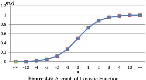
Figure 4.6: A graph of Logistic Function ... 34

Figure 4.7: Histogram Examples ... 64

Figure 4.8: Density Plot Examples ... 65

Figure 5.1: Commands to achieve Statistical measures for “NdarExposure.txt” ... 68

Figure 5.2: Commands to achieve Histograms for “NdarExposure.txt”... 70

Figure 5.3: Histogram of some attributes(a) ... 71

Figure 5.4: Histogram of some attributes(b) ... 72

Figure 6.1: Scatter plots of linearly related variables with log-odds ... 91

(17)

viii

LIST OF ABBREVIATIONS

ASD Autism spectrum disorder

CDC Centers for Disease Control and Prevention

ADDM The Autism and Developmental Disabilities Monitoring WHO World Health Organization

TRAP Traffic-related air pollution HAP Hazardous air pollutant

NDAR National Database repository for Autism Research ADHD Attention deficit hyperactivity disorder

CHD Coronary Heart Disease

MLE Maximum Likelihood Estimation AIC Akaike Information Criterion BIC Bayesian information criterion LRT Likelihood Ratio Test

LR Likelihood Ratio GOF Goodness Of Fit IQR Interquartile Range

NIH National Institutes of Health AOR Adjusted Odds Ratio

(18)

1

1. INTRODUCTION

1.1 Background to the Study

Autism spectrum disorder (ASD) is considered as a group of neurodevelopmental disorder that is characterized by difficulties with communication and social interaction and restricted, repetitive and stereotyped behaviors, interests, and activities present in early childhood [1, 2]. The prevalence of ASD was estimated 1 in 59 in the US according to the CDC’s ASD prevalence report [3] in April 2018 and was 4 times more common in boys than girls. It also showed a dramatic rise, approximately from 0.67 (1 in 150) in 2002 to 1.69 (1 in 59) in 2014 [4]). The symptoms are generally evident in the early developmental life of a child, usually 2-3 years old and many children are not diagnosed as soon as the baby is born.

Recently, many researchers have been trying to find out the causes of ASD, but they couldn’t find the exact causes of ASD. Epidemiological studies suggest that both genetics and environment likely play a role in ASD [5, 6]. The environmental factors were suggested to account for around 40% for autism [7, 8]. Similarly, the genetic factors are responsible for around 50% of the risk for ASD [8]. So, some studies have demonstrated that understanding the contribution of environmental factors to ASD might be easier than genetics and helpful on the increasing prevalence of ASDs [9].

1.2 Statement of the Problem and Motivation

The recent increase in brain disorders such as ASD, ADHD, and Down syndrome and the birth of my nephew with Down syndrome have motivated me to work on these issues. I asked myself “Why the prevalence of autism has increased without sufficient explanation and what can I do?”

(19)

2

When we think about what is going on parallel in the world with the rise of autism, it can be seen that the environment is excessively polluted by toxic wastes caused by urbanization, industrialization, and increase in the transportation due to globalization, that is, increase in the number of vehicles.

So, environmental factors or exposures including all nongenetic factors, from viruses and medications to chemicals agents during prenatal, natal, and postnatal development may influence brain development, leading to neurodevelopmental abnormalities that can contribute to ASD [7].

Researcher have noted several environmental risk factors related to ASD before and during birth, such as increased maternal and paternal age, maternal health during pregnancy, maternal lifestyle, pregnancy complications and prenatal exposure to environmental toxins(heavy metals, pesticides, industrial pollutants, and air pollution)

As a result, in my study, as a criminal of autism, air toxins that pollute the environment, especially traffic-related pollution (TRAP) made me motivated to study ASD despite the genetic susceptibility.

1.3 Objectives

This study aims to investigate the relation between traffic-related air pollution (TRAP) and four air pollutants (NO2, O3, PM10, PM2.5) and ASD during prenatal or post-natal

1.4 Methodology

The available data for my research has been collected from the National Database repository for Autism Research (NDAR) data repository [10].

My working data is a collection whose title is “Distance to Freeway and Major Road” and its investigator is Rob McConnell. This collection contains birth address-based measures on the distance to the interstate highway, state highway, major road, and local

(20)

3

road for study subjects enrolled in the CHARGE study, and the subjects for this project were pregnant mothers.

Multiple logistic regression was used to test the relation between air pollutants (NO2,

O3, PM10, PM2.5) and ASD.

The likelihood ratio and Wald test were used to illustrate how the significance of regression parameters in multiple logistic regression.

Since the number of explanatory variables is large (i.e., 40 or more), variable selection methods were used to choose the best subset of the predictors among many variables associated with the outcome.

1.5 Significance of the Study

The early years of a child’s life particularly the period from birth to 2 years old are very important for brain development. The brain grows incredibly in two years. 80% of brain development is completed in this period. During this stage, children are highly influenced by the environment. Many factors in addition to genes such as inadequate nutrition and exposure to toxins or infections during and after pregnancy affect brain development. This period is likely to be critical in neurodevelopmental disorders including autism [11, 12].

So, the first reason why this study is important for me is that I focused on the air pollutant exposures from four different roads occurring from the first trimester through the child’s first year which are the periods of brain development. Secondly, we tried to make clear the role of timing for TRAP during pregnancy and early life and tested the relation between TRAP and ASD. Finally, identifying air pollutant exposures that contribute to autism is important to prevent ASD by reducing ambient pollution with the help of government policies and therefore informing a large number of people especially sensitive groups of pregnant women and children.

(21)

4

1.6 Organization of Study

In this project, the data mining techniques were used according to CRISP-DM, in which a given data mining project has a life cycle consisting of six phases, as illustrated in Figure 1.1. Note that the iterative nature of CRISP is symbolized by the outer circle, the significant dependencies between phases are indicated by the arrows. The phase sequence can be changed due to different conditions. That is, the next phase in the sequence often depends on the outcomes associated with the previous phase [13].

Figure 1.1: Cross-Industry Standard Process for Data Mining (CRISP-DM) [13]

The organization of this thesis as follows:

Chapter 1 deals with the background of the study (ASD and causes), statement of the problem (motivation), objectives of the study, methodology, and significance of the study.

Chapter 2 introduces the ASD domain, what ASD is, its causes and prevalence, and environmental factors playing role in ASD. It also examines the related literature review.

(22)

5

Chapter 3 is a data understanding phase that describes the source of data, datasets, and data fields.

Chapter 4 gives the theoretical background, the applied data preprocessing, logistic regression, and variable selection methods.

Chapters 5 covers the analysis of data and evaluates the quality of the data, cleaning the raw data, and dealing with missing and outlier data before proceeding to the modeling phase.

Chapter 6 covers model building and model evaluation phases. It presents the implementation of logistic regression, how to fit the logistic regression model, how to teste the significance of coefficients, and interpret the model coefficients. Additionally, it describes the variable selection methods and provides the results for each model in the study.

Chapter 7 presents a summary of the main findings achieved in Chapter 6.

(23)

6

2. AUTISM & LITERATURE REVIEW

2.1 What is Autism?

Autism spectrum disorder (ASD) is a group name given to a collection of neurodevelopmental disorders such as Autistic Disorder, Childhood Disintegrative Disorder, Asperger Syndrome, Rett’s Disorder, and Pervasive Developmental Disorder. Its symptoms and characteristics can be described as a lack of social dialog with other people, lack of communication skills, repetitive, stereotypical attitudes, body movements especially appearing in the early developmental life of a child. These symptoms and characteristics can occur in different combinations and degrees ranging from mild to severe and also no two Autistic children resemble each other [14, 10, 15].

2.2 Prevalence of ASD

Autism prevalence shows how common ASD is in the general population. In the United States, an ASD prevalence estimates report [16] was published by the Centers for Disease Control and Prevention (CDC) in 2018. The report subjects’ data whose records of 8 years old children living in 11 areas of the United States were collected by The Autism and Developmental Disabilities Monitoring (ADDM) Network surveillance system during 2014. The summary of the ASD prevalence report is shown in Table 2.1 [17].

(24)

7

Table 2.1: Prevalence of ASD in 8-year-olds (2014) [18]. Prevalence 1 in x Prevalence % Sex Boys 1 / 38 2.70% Girls 1 / 152 0.70% Race / Ethnicity White 1 / 58 1.70% Black 1 / 63 1.60%

Asian / Pacific Islander 1 / 74 1.40%

Hispanic 1 / 71 1.40%

Overall 1 / 59 1.70%

According to Table 2.1,

 The overall average prevalence of ASD 1 in every 59

 ASD is 4 times more common in boys than girls. For example, it is 0.7% for girls, whereas 2.7% in boys.

 ASD occurs in the children of different races and ethnic groups and the prevalence for non-Hispanic white children is higher than non-Hispanic black children.

The results of many studies conducted in Asia, Europe, and North America were found to be between 1% and 2% for average prevalence [19]. The estimated prevalence of ASD with the collected data of the children living in 11 different sites between 2000 and 2014 years across the US are shown in Table 2.2 [19]. It is concluded that the estimated prevalence of ASD increased by approximately 16% between 2012 and 2014, 25% between 2006 and 2008, 71% between 2002 and 2008, and 100% between 2004 and 2014.

(25)

8

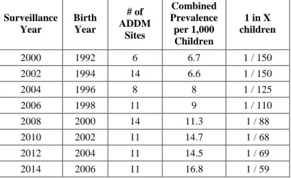
Table 2.2: Prevalence of ASD based on ADDM Network studies published from 2007

to 2018 (surveillance years 2000-2014) [19]. Surveillance Year Birth Year # of ADDM Sites Combined Prevalence per 1,000 Children 1 in X children 2000 1992 6 6.7 1 / 150 2002 1994 14 6.6 1 / 150 2004 1996 8 8 1 / 125 2006 1998 11 9 1 / 110 2008 2000 14 11.3 1 / 88 2010 2002 11 14.7 1 / 68 2012 2004 11 14.5 1 / 69 2014 2006 11 16.8 1 / 59

Based on the data in Table 2.2 dramatic increases in the prevalences of ASD can be seen in Figure 2.1

Figure 2.1: The Estimated ASD Prevalence Rate (per 1000) based on Table 2.2 Data

Finally, while ASD was a rare disease, now it is 1 in 59 among children. Why this dramatic growth has been? It may be explained with better diagnosis and more advanced diagnostic criteria [20].

1 in 150 1 in 150 1 in 125 1 in 110 1 in 88 1 in 68 1 in 69 1 in 59 0 2 4 6 8 10 12 14 16 18 20 2000 2002 2004 2006 2008 2010 2012 2014 Esti m ate d AS D Pr e val e n ce R ate (p e r 1000 ) Survilance Years

(26)

9

2.3 Causes and Risk Factors

Recently, increasing autism prevalence rates have been found in many studies without enough explanation about it. Although scientists are still trying to understand the causes of ASD, they couldn’t manage to identify the exact causes of autism. There may be many risk factors that can cause a child more likely to have an ASD. It is generally believed that genetics and environmental factors both play a role in ASD [5, 6].

Genetic risk factors are present at birth especially in DNA such as gene mutations, gene deletions, or duplications, however environmental risk factors or all non-genetic factors may cause to develop ASD during prenatal or postnatal periods [21].

2.3.1 Genetic Factors

Many researcher believe that there is a strong role of genes in the development of ASD [22]. Twin and family studies support the genetic theory [23]. For example, ASD is 50 to 200 times more common in siblings of autistic probands than normal population [22] and, parents who have a child with ASD have a 2%–18% chance of a second affected child [24]. While the contribution of genetic factors to ASD was 7–8% of autism cases in 2010 [25], but this contribution has increased about 10-30% with the help of higher diagnostic tools [26].

2.3.2 Environmental Factors

The environment can be defined as a combination of external physical factors that affect the development of a child. These factors can be either viruses, medications or chemicals, and physical agents [27]. In fact, the first environment for a child is the womb in which the baby develops, and it is involved in the development of autism. Environmental factors may influence brain development at different stages. They act together in harmony with susceptible genes. They are some interactions with each other, which may lead to changes in gene expression. Additionally, genes may indirectly change the biochemistry of the brain by affecting the metabolism and activity of foreign

(27)

10

chemicals such as pesticides. Changes to DNA, not inherited from parents, causing damage to the genetic code environmental exposures are associated with ASD risk [27]. Scientists believe that de novo mutations lead to some children to susceptible to ASD when exposed to certain environmental factors [28].

Environmental factors are thought to be responsible for around 40% for ASD and 10– 40% of the risk for ADHD [29].

Changes in over 1,000 genes have been thought to affect the risk of developing ASD, but most of these variations have only a small effect when combined with environmental risk factors, such as increased maternal age, pregnancy complications, and others that have not been identified. “Non-genetic factors may contribute up to about 40 percent of ASD risk” [30].

The different environmental risk factors may be associated with ASD involves events before and during birth, such as

 Increased maternal and paternal age

 Maternal Health during pregnancy (Maternal stress, maternal obesity, diabetes or immune factors)

 Maternal Lifestyle (Medication usage such as prenatal vitamins and folic acid and related nutrients, substance use, drug usage, alcohol usage, and smoking)

 Pregnancy complications

 Metabolic complications like gestational diabetes,

 Delivery complications such as birth asphyxia leading to oxygen deprivation of the baby’s brain,

 Neonatal complications such as low birth weight, preterm birth.

 Prenatal or postnatal exposure to environmental toxins

 Heavy metals such as lead and mercury,

 Pesticides such as organophosphate pesticides (OPs) or organochlorines pesticides (OCPs),

(28)

11

 Industrial Pollutants like Phthalates or Polychlorinated Biphenyls(PCB),

 Air pollution such as hazardous air pollutants(benzene, methylene chloride), criteria air pollutants (NO2, O3, PM2.5, PM10), metals(lead,

cadmium), and traffic-related pollution (TRAP) [27, 31].

In my study, criteria air pollutants (especially NO2, O3, PM2.5, PM10), and TRAP were

focused due to the working datasets.

2.3.2.1 Air pollution

Air pollution which is also called air toxics or air pollutants is a combination of many kinds of gases, droplets, and solid particles in the air. Because of the increase in population and the need for energy, it has become a very important problem all over the world [32, 33, 34].

Air pollution has been mostly caused by the air toxics emitted from different sources, primarily transportation(e.g., automobile, trucks, buses exhaust), secondly industrial emissions (e.g., factories, refineries, power generation) and thirdly indoor sources(e.g. smoking, cooking, heating, and lighting, vapors from building materials, paints)

[35, 36, 37].

There are many types of air pollutants, but the major ones that make the air quality worse are particulate matter (PM), sulfur dioxide (SO2), carbon monoxide (CO),

nitrogen dioxide (NO2), ozone (O3) and lead [38].

According to the World Health Organization (WHO) statistics reports that around 7 million people die every year from exposure to polluted air [39]. Additionally, hazardous air pollutants (HAPs) have negative impacts on health, they may cause cancer or other serious health effects, such as neurological or respiratory disease and birth or developmental defects[38].

(29)

12

There is increasing evidence that TRAP which is emitted by vehicles especially in urban areas contributes to air quality and may affect pregnancy outcomes and child development [40, 41].

It has been reported that the emissions caused by the transportation sector are approximately 55%, 10%, and 10% for NOx, VOCs, and PM2.5 and PM10 respectively

in the U.S [41].

The traffic-related air pollutants (NO2, NO, O3, SO2, CO, and PM) were mainly focused

on in these studies. Most of the studies showed a positive association between maternal exposure to the abovementioned pollutants and ASD.

In 2011, Volk et al. [1] investigated the relationship between distance to the major roads of the children’s homes and ASD. Children who lived within 309m of a freeway have higher odds of having autism than children who lived bigger than 1149 m from a freeway [1]. Further, in 2013, Volk et al. [2] further discovered that exposure to TRAP, NO2, PM2.5, and PM10 during the first year of life was associated with autism.

2.3.2.1.1 Nitrogen Oxides (NOx)

Nitrogen oxides (NOx) are a group of gases that are composed of nitrogen(N) and

oxygen (O). Two of the most common nitrogen oxides are nitric oxide (NO) and nitrogen dioxide (NO2). Nitrogen oxides are emitted from motor vehicle exhaust and

high-temperature combustion processes such as power plants or industrial plants by burning of coal, oil, diesel fuel, and natural gas.

Particulate matter and ground-level ozone are formed by the reaction NOx with sunlight

or other chemicals in the air. Acid rains are also formed by the end of the interaction of NOx with water, oxygen, and other chemicals(eg., sulfur dioxide) in the atmosphere.

If you live near power or industrial plants or if you are in heavy traffic, further if you smoke cigarettes, you can be exposed to nitrogen oxides by breathing air [42, 43].

(30)

13

There have been some studies finding the relation between ASD and NO2 in literature.

In 2013, Volk et al. [2] found that exposure to nitrogen dioxide during gestation was also associated with ASD. Then, Ritz et al. [44] found NO2 exposure in all trimesters to

be associated with ASD in 2018. Finally, in 2109, Oudina et al. [4], found that exposure to nitrogen dioxide during the prenatal period was associated with autism. On the other hand, Gong et al. [3], Gong et al. [45], Pagalan et al. [46], Raz et al. [34] studies reported no associations.

2.3.2.1.2 Particulate Matter

Particulate matter (PM) is a mixture of solid or liquid tiny particles suspended in the air which are approximately 1 to 10 micrometers(µm) in size.

The Particulate matter (PM) is identified according to aerodynamic diameter  PM10: inhalable coarse particles with a diameter smaller than 10 µm  PM2.5: fine inhalable small particles with a diameter smaller than 2.5 µm

Many particles are emitted into the atmosphere from transportation (vehicles), industry (factory), combustion of fossil fuels, natural (e.g. by dust storms). These particles are also formed in the atmosphere as a result of complex chemical reactions between pollutants such as sulfur dioxide and nitrogen oxide.

Since these particles are very small, they are more dangerous when breath, they may reach inside the lungs. They have important effects on human health, such as cardiovascular, lung, skin diseases, and sometimes cause premature deaths [34, 37, 47, 48].

PM2.5 were positively associated with ASD in the following studies:

Becerra et al. [37] and Volk et al. [2] in 2013, Talbott et al. [49] and Raz et al.[39] in 2015, Chen et al. [50] and Ritz et al. [44] in 2018, Geng et al. [51] and Jo et al. [52] in 2019.

(31)

14

However, in 2 other studies, Guxens et al.[53] and Pagalan et al. [54], found no association between ASD and PM2.5, even though their study populations also consisted

of Californian children.

PM10 was positively associated with ASD in the following studies:

Volk et al. [2] in 2013, Kalkbrenner et al. [55] in 2015, Kim et al. [56] in 2017, Chen et al. [50] in 2018.

In contrast, the following studies found no association between PM10 and ASD:

Gong et al. [3], Guxens et al. [53], Gong et al. [45], Ritz et al. [44], Yousefian et al. [57].

2.3.2.1.3 Ozone

Ozone (O3) is a natural gas molecule made up of three oxygen atoms joined together.

Ozone can be classified as Good and Bad Ozone. Good ozone is found naturally in the upper Stratosphere which forms an ozone layer around the Earth and protects from the sun's harmful ultraviolet radiation by absorbing them. On the other hand, Bad or ground-level ozone is found in the Troposphere where the lowest layer of Earth's atmosphere. It does not exist naturally but is mainly formed through chemical reactions between nitrogen oxides (NOx) and volatile organic compounds (VOC) when sunlight reacts with the pollutants emitted from the human activities (e.g, vehicles, power plants, factories, refineries, etc.).

Ground-level ozone is the major component of “smog”. It is very harmful to humans and plants life because it contaminates the air and oxidizes biological tissues.

Someone can be exposed to unhealthy highest levels of Ozone on hot sunny days in urban areas while exercising or working outdoors in the middle of the day.

Exposure to ozone may damage the lungs and reduce lung function especially in developing children. Additionally, it may give damage to a fetus and may increases the

(32)

15

risk of premature death, especially in people having heart and lung disease [58, 59, 60, 34, 37].

In, Becerra et al. [37] and Jung et al. [61] in 2013 studies, the relation between ASD and Ozon(O3) is found. However, Volk et al. [2], Kerin et al. [62], Kaufman et al. [63] found no associations between ASD and Ozon (O3).

(33)

16

3. DATA

3.1 Data Collection

The data used in this thesis has been collected from the National Database repository for Autism Research (NDAR) data repository which is developed by The National Institutes of Health (NIH) [64].

Researchers requesting to access data contained in NDAR Collections, first of all, should submit data use certification DUC and this submission should be approved by Data Access Comite (DAC). This request procedure takes a little bit of time.

3.2 Datasets

The data documents which are in text format with the titles shown in Table 3.1 are downloaded from the NDAR data repository [64], by first logging in and clicking Data Dictionary [65] then searching and filtering for the “Exposure” category. Table 3.1 shows the information about the datasets in “Distance to Freeway and Major Road Data” Collection.

Table 3.1: Distance to Freeway and Major Road Data Collection

No Datasets Title Txt Files Number of

Subjects

Number Of Records

1 Traffic Related Air Pollution (TRAP) Estimates trp_estimates01 1039 6206

2 Distance to Roadways roaddistance02 1049 1049

3 Nitrogen Dioxide (NO2) Exposure no2_exposure01 1049 6284

4 Ozone(O3) Exposures o3_exposure01 1049 6284

5 Particulate Matter 10 (PM10) Exposures pm10_exposures01 1049 6284

(34)

17

The working data is a collection with the title “Distance to Freeway and Major Road” and whose investigator is Rob McConnell. The data in these collections belong to the CHARGE study of pregnant mothers. It contains the measure of some exposures estimated according to the distance to some roads. The subjects enrolled in the CHARGE study in the above data collections, shown below, includes also both pregnant mother and their child info. The phenotype of the child is associated with the mother's data. CHARGE subjects were preschool children between 24 and 60 months of age and were born between 1997 and 2006 in California when they joint with the organization.

The exposures measures were estimated for each trimester of pregnancy and the first year of life by using the mother’s address and the Environmental Protection Agency’s Air Quality System data [2].

The information contained in these datasets are:

 Traffic-related air pollution (TRAP) estimate: dataset contains traffic-related air pollution (TRAP) estimate averages for 5 time periods. They are constructed based on mothers’ address locations. The concentrations of nitrogen oxides from freeways, non-freeways, and all roads located within 5 km of each child’s home are estimated by using the CALINE-4 line source dispersion model. Here, nitrogen oxides (NOx) concentrations can be viewed as an indicator of the TRAP mixture since they showed a perfect correlation with other traffic-related pollutants before [2].

 Distance to Roadways: contains the distances (in meters) to nearest class-1,

class-2, class-3, and class-4 roads to subjects birth residence(on birth address)  Nitrogen Dioxide (NO2) Exposure: contains NO2 estimated averages for 5 time

periods. Nitrogen oxides (NOx) concentrations can be viewed as an indicator of the TRAP mixture since they showed a perfect correlation with other traffic-related pollutants.

 Ozone (O3) Exposures: contains ozone estimated averages for 5 time periods

 Particulate Matter 10 (PM10) Exposures: contains PM10 estimated averages for

(35)

18

 Particulate Matter 2.5 (PM2.5) Exposures: contains PM2.5 estimated averages

for 5 times.

Where exposure during 6 time periods under study includes:  Preg: All pregnancy,

 Trim1: First trimester,  Trim2: Second trimester,  Trim3: Third trimester.  1stYr: First year,  2ndYr: Second year.

and road type and their definitions are given as:  Class-1: Interstate highway

 Class-2: the US and state highways

 Class-3: Secondary state or county highway

 Class-4: Local, neighborhood, rural road, city street

The exposure measurements for PM2.5, PM10, O3, and NO2 were estimated from the US

EPA’s Air Quality System (AQS) data by using the regional air quality data [2].

3.3 Data fields of the Datasets

“Traffic-Related Air Pollution (TRAP) Estimates”, “Distance to Roadways” “Nitrogen Dioxide (NO2) Exposures”, “Ozone(O3) Exposures”,

“Particulate Matter 10 (PM10) Exposures”, “Particulate Matter 2.5 (PM2.5) Exposures” dataset attributes were shown in Table 3.2, Table 2.3, Table 3.4, Table 2.5, Table 3.6, and Table 3.7 respectively.

(36)

19

Table 3.2: “Traffic-Related Air Pollution (TRAP) Estimates” Table Attributes

No Attribute Name Description

1 Subject_key The NDAR Global Unique Identifier (GUID) for research subject

2 gender Gender

3 phenotype Phenotype/diagnosis for the subject

4 periodname Time Period for Exposure(Preg,Trim1,Trim2,Trim3,1stYr,2ndYr)

5 roadtype1_nox Avg. NOx in ppb estimate from Interstate Highways 6 roadtype2_nox Avg. NOx in ppb estimate for US and State Highways

7 roadtype3_nox Avg. NOx in ppb estimate for secondary state or county highways

8 roadtype4_nox Avg. NOx in ppb estimate for local, neighborhood, rural road, or city street 9 roadtypeAll_nox Avg. NOx in ppb estimate from all road types

Table 3.3: “Distance to Roadways” Table Attributes

No Attribute Name Description

2 gender Gender

4 fcc1_distance Distance (in meters) to the nearest class-1 road to the birth residence

Table 3.4: “Nitrogen Dioxide (NO2) Exposures” Table Attributes

2 gender Gender

5 no2_exposure Avg. NO2 in ppb

Table 3.5: “Ozone(O3) Exposures” Table Attributes

2 gender Gender

4 periodname Time Period for Exposure

(Preg,Trim1,Trim2,Trim3,1stYr,2ndYr)

(37)

20

Table 3.6: “Particulate Matter 10 (PM10) Exposures” Table Attributes

2 gender Gender

5 pm10 Avg. exposure to PM 10 in ppb

Table 3.7: “Particulate Matter 2.5 (PM2.5) Exposures” Table Attributes

2 gender Gender

4 periodname Time Period for

Exposure(Preg,Trim1,Trim2,Trim3,1stYr,2ndYr)

5 pm25 Avg. PM 2.5 in ppb (part per billion)

All the tables in Table 3.1 were imported to new tables in Microsoft Access. Then, “Nitrogen Dioxide (NO2) Exposures”, “Ozone(O3) Exposures”,

“Particulate Matter 10 (PM10) Exposures” and “Particulate Matter 2.5 (PM2.5)

Exposures” tables were also transformed and transposed into new temporary tables such

as tempNO2, tempO3, tempPM10 and temp25 respectively with a large number of rows but a small number of dimensions as in Table 3.8 and Table 3.9.

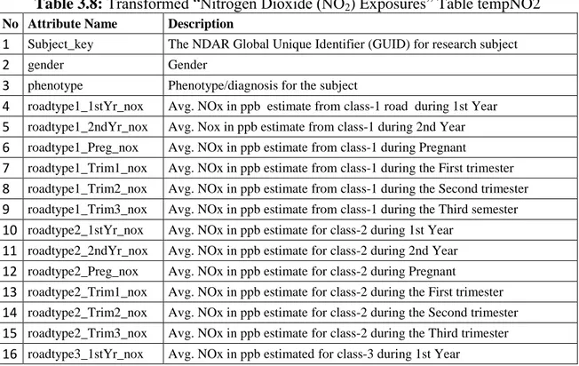
Table 3.8: Transformed “Nitrogen Dioxide (NO2) Exposures” Table tempNO2

2 gender Gender

4 roadtype1_1stYr_nox Avg. NOx in ppb estimate from class-1 road during 1st Year

5 roadtype1_2ndYr_nox Avg. Nox in ppb estimate from class-1 during 2nd Year

6 roadtype1_Preg_nox Avg. NOx in ppb estimate from class-1 during Pregnant

7 roadtype1_Trim1_nox Avg. NOx in ppb estimate from class-1 during the First trimester

8 roadtype1_Trim2_nox Avg. NOx in ppb estimate from class-1 during the Second trimester

9 roadtype1_Trim3_nox Avg. NOx in ppb estimate from class-1 during the Third semester

10 roadtype2_1stYr_nox Avg. NOx in ppb estimate for class-2 during 1st Year

11 roadtype2_2ndYr_nox Avg. NOx in ppb estimate for class-2 during 2nd Year

12 roadtype2_Preg_nox Avg. NOx in ppb estimate for class-2 during Pregnant

13 roadtype2_Trim1_nox Avg. NOx in ppb estimate for class-2 during the First trimester

14 roadtype2_Trim2_nox Avg. NOx in ppb estimate for class-2 during the Second trimester

15 roadtype2_Trim3_nox Avg. NOx in ppb estimate for class-2 during the Third trimester

(38)

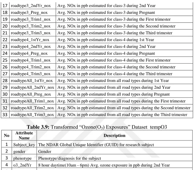
21

17 roadtype3_2ndYr_nox Avg. NOx in ppb estimated for class-3 during 2nd Year

18 roadtype3_Preg_nox Avg. NOx in ppb estimated for class-3 during Pregnant

19 roadtype3_Trim1_nox Avg. NOx in ppb estimated for class-3 during the First trimester

20 roadtype3_Trim2_nox Avg. NOx in ppb estimated for class-3 during the Second trimester

21 roadtype3_Trim3_nox Avg. NOx in ppb estimated for class-3 during the Third trimester

22 roadtype4_1stYr_nox Avg. NOx in ppb estimated for class-4 during 1st Year

23 roadtype4_2ndYr_nox Avg. NOx in ppb estimated for class-4 during 2nd Year

24 roadtype4_Preg_nox Avg. NOx in ppb estimated for class-4 during Pregnant

25 roadtype4_Trim1_nox Avg. NOx in ppb estimated for class-4 during the First trimester

26 roadtype4_Trim2_nox Avg. NOx in ppb estimated for class-4 during the Second trimester

27 roadtype4_Trim3_nox Avg. NOx in ppb estimated for class-4 during the Third trimester

28 roadtypeAll_1stYr_nox Avg. NOx in ppb estimated from all road types during 1st Year

29 roadtypeAll_2ndYr_nox Avg. NOx in ppb estimated from all road types during 2nd Year

30 roadtypeAll_Preg_nox Avg. NOx in ppb estimated from all road types during Pregnant

31 roadtypeAll_Trim1_nox Avg. NOx in ppb estimated from all road types during the First trimester

32 roadtypeAll_Trim2_nox Avg. NOx in ppb estimated from all road types during the Second trimester

33 roadtypeAll_Trim3_nox Avg. NOx in ppb estimated from all road types during the Third trimester

Table 3.9: Transformed “Ozone(O3) Exposures” Dataset tempO3

No Attribute

Name Description

2 gender Gender

4 o3_2ndYr 8 hour daytime(10am - 6pm) Avg. ozone exposure in ppb during 2nd Year

5 o3_Preg 8 hour daytime(10am - 6pm) Avg. ozone exposure in ppb during Pregnant

6 o3_Trim1 8 hour daytime(10am - 6pm) Avg. ozone exposure in ppb during the First trimester

7 o3_Trim2 8 hour daytime(10am - 6pm) Avg. ozone exposure in ppb during the Second trimester

8 o3_Trim3 8 hour daytime(10am - 6pm) Avg. ozone exposure during the Third trimester

Then, a new “Exposure” table was created by joining tempNO2, tempO3, tempPM10, and temp25 tables with the “subject key” field and inserting their data into the “Exposure” table. The newly formed “Exposure” table shown in Table 3.10 consists of 1039 records or instances corresponding to a single subject. It contains a total of 61 separate data fields having 1 text, 2 categorical, 59 numerical fields. Details of the fields are given in Table 3.10.

(39)

22

Table 3.10: “Exposure” Dataset Attributes

2 gender Gender

4 fcc1_distance Distance (in meters) to the nearest class-1 road to the birth residence 5 fcc2_distance Distance (in meters) to the nearest class-2 road to the birth residence 6 fcc3_distance Distance (in meters) to the nearest class-3 road to the birth residence 7 fcc4_distance Distance (in meters) to the nearest class-4 road to the birth residence 8 roadtype1_1stYr_nox Avg. NOx in ppb estimate from class-1 road during 1st Year 9 roadtype1_2ndYr_nox Avg. Nox in ppb estimate from class-1 during 2nd Year 10 roadtype1_Preg_nox Avg. NOx in ppb estimate from class-1 during Pregnant

11 roadtype1_Trim1_nox Avg. NOx in ppb estimate from class-1 during the First trimester 12 roadtype1_Trim2_nox Avg. NOx in ppb estimate from class-1 during the Second trimester 13 roadtype1_Trim3_nox Avg. NOx in ppb estimate from class-1 during the Third semester 14 roadtype2_1stYr_nox Avg. NOx in ppb estimate for class-2 during 1st Year

15 roadtype2_2ndYr_nox Avg. NOx in ppb estimate for class-2 during 2nd Year 16 roadtype2_Preg_nox Avg. NOx in ppb estimate for class-2 during Pregnant

17 roadtype2_Trim1_nox Avg. NOx in ppb estimate for class-2 during the First trimester 18 roadtype2_Trim2_nox Avg. NOx in ppb estimate for class-2 during the Second trimester 19 roadtype2_Trim3_nox Avg. NOx in ppb estimate for class-2 during the Third trimester 20 roadtype3_1stYr_nox Avg. NOx in ppb estimated for class-3 during 1st Year

21 roadtype3_2ndYr_nox Avg. NOx in ppb estimated for class-3 during 2nd Year 22 roadtype3_Preg_nox Avg. NOx in ppb estimated for class-3 during Pregnant

23 roadtype3_Trim1_nox Avg. NOx in ppb estimated for class-3 during the First trimester 24 roadtype3_Trim2_nox Avg. NOx in ppb estimated for class-3 during the Second trimester 25 roadtype3_Trim3_nox Avg. NOx in ppb estimated for class-3 during the Third trimester 26 roadtype4_1stYr_nox Avg. NOx in ppb estimated for class-4 during 1st Year

27 roadtype4_2ndYr_nox Avg. NOx in ppb estimated for class-4 during 2nd Year 28 roadtype4_Preg_nox Avg. NOx in ppb estimated for class-4 during Pregnant

29 roadtype4_Trim1_nox Avg. NOx in ppb estimated for class-4 during the First trimester 30 roadtype4_Trim2_nox Avg. NOx in ppb estimated for class-4 during the Second trimester 31 roadtype4_Trim3_nox Avg. NOx in ppb estimated for class-4 during the Third trimester 32 roadtypeAll_1stYr_nox Avg. NOx in ppb estimated from all road types during 1st Year 33 roadtypeAll_2ndYr_nox Avg. NOx in ppb estimated from all road types during 2nd Year 34 roadtypeAll_Preg_nox Avg. NOx in ppb estimated from all road types during Pregnant

35 roadtypeAll_Trim1_nox Avg. NOx in ppb estimated from all road types during the First trimester 36 roadtypeAll_Trim2_nox Avg. NOx in ppb estimated from all road types during the Second trimester 37 roadtypeAll_Trim3_nox Avg. NOx in ppb estimated from all road types during the Third trimester 38 no2_1stYr Avg. NO2 in ppb during 1st Year

39 no2_2ndYr Avg. NO2 in ppb during 2nd Year 40 no2_Preg Avg. NO2 in ppb during Pregnant

(40)

23

42 no2_Trim2 Avg. NO2 in ppb during the Second trimester 43 no2_Trim3 Avg. NO2 in ppb during the Third trimester 44 o3_1stYr Avg. ozone exposure in ppb during 1st Year

45 o3_2ndYr 8 hour daytime(10am - 6pm) Avg. ozone exposure in ppb during 2nd Year 46 o3_Preg 8 hour daytime(10am - 6pm) Avg. ozone exposure in ppb during Pregnant 47 o3_Trim1 8 hour daytime(10am - 6pm) Avg. ozone exposure in ppb during the First _trimester 48 o3_Trim2 8 hour daytime(10am - 6pm) Avg. ozone exposure in ppb during the

Second trimester

49 o3_Trim3 8 hour daytime(10am - 6pm) Avg. ozone exposure during the Third trimester

50 pm10_1stYr Average exposure to PM 10 in ppb during 1st Year 51 pm10_2ndYr Average exposure to PM 10 in ppb during 2nd Year 52 pm10_Preg Average exposure to PM 10 in ppb during Pregnant

53 pm10_Trim1 Average exposure to PM 10 in ppb during the First trimester 54 pm10_Trim2 Average exposure to PM 10 in ppb during the Second trimester 55 pm10_Trim3 Average exposure to PM 10 in ppb during the Third trimester 56 pm25_1stYr Average PM 2.5 in ppb during 1st Year

57 pm25_2ndYr Average PM 2.5 in ppb during 2nd Year 58 pm25_Preg Average PM 2.5 in ppb during Pregnant

59 pm25_Trim1 Average PM 2.5 in ppb during the First trimester 60 pm25_Trim2 Average PM 2.5 in ppb during the Second trimester 61 pm25_Trim3 Average PM 2.5 in ppb during the Third trimester

The summary of the subjects in “Exposure” table was shown in Table 3.11

Table 3.11: The distribution of the subjects in “Exposure” Dataset

Phenotype # of

Subjects

AUTISM SPECTRUM AFFECTED 141

AUTISM SPECTRUM SEVERELY AFFECTED 338

NEUROLOGICAL CONTROL 136

NOT DEFINED 152

TYPICAL CONTROL 272

TOTAL 1039

There are some mechanisms and rules used for phenotype categorization when they are shared data in NDAR. Subjects Categorization is performed based upon the following order:

1. Fragile X 2. Controls

(41)

24

 Non-Spectrum Typical Control (e.g. typical, sibling, parent)  Non-Spectrum Neurological Control

3. Autism Spectrum  Severely Affected  Mildly Affected  Affected

Fragile X is defined according to provided genetic test results for the Fragile X mutation of the FMR1 gene.

Typical controls are typically developing individuals. The Neurological disorders sub‐phenotype control group includes subjects with a learning disability, Attention Deficit Hyperactivity Disorder, developmental disability, intellectual disability/MR, or other neurological disorders, excluding Fragile X and subjects with positive genetic test result for Non‐Spectrum Neurological conditions.

NDAR categorizes Typical and Neurological Disorder control subjects based on results from the ADI‐R, ADOS, IQ, and Vineland Survey assessments. NDAR also categorizes the AUTISM SPECTRUM AFFECTED, AUTISM SPECTRUM SEVERELY AFFECTED phenotypes according to cut-offs, for each Assessment (ADI‐R, ADOS, IQ, and Vineland Survey). Note that a minimum of three assessments ‐including ADI‐R and ADOS – plus one other measure (Vineland or an IQ) is needed for the categorization of an autism spectrum phenotype. 'Not defined" means that not enough data provided to define phenotype. In the absence of a diagnosis, NDAR categorizes control subjects based on the results from the ADI-R, ADOS, IQ, and Vineland Survey assessments.

(42)

25

4. METHODS

4.1 Data Preprocessing

Data preprocessing is an important phase of the data mining process which aims to improve data quality and efficiency of the data mining process. Since the real world row data is not perfect and dirty, it modifies the data to make it more suitable and transforms raw data into an understandable format for data analysis [66, 13].

Most of the analyzed raw data have generally common data quality problems

 Completeness: Not all attributes in the data table have correct values for missing value and some records might have missing values because of some technical reasons. For example , a survey might be filled out by skipping age information.  Accuracy: It refers to the deviation of the data value from the true or expected value. For numerical attributes, out of range values or the reduction in the correctness of the data can be caused by noise or wrong measurements.

 Inconsistent: Inconsistent values in data occur when entering wrong codes or

information instead of what should be. Let’s say, the user entered birthday to be May 07, 1993, and the age attribute displays 50.

The major steps involved in data preprocessing are data cleaning and data transformation. They are useful for the databases that need to preprocessing. Data preprocessing can be responsible for 10–60% of time and effort in the whole data mining process [13].

(43)

26

4.1.1 Data Cleaning

Data cleaning is a process that improves data quality. It involves filling in missing values, correction of simple errors, correcting inconsistencies, removing noise, duplicate records, and outliers [67, 66]. It is a necessary time-consuming procedure and needs serious effort for successful data mining [68].

4.1.1.1 Handling Missing Values

Missing data may stem from many different causes. While analyzing data, it is quite often encountered that no data value is stored in certain records for some of the attributes quite often occur in datasets. For example, a sensor may be defective and may not send healthy data, or some participants in a survey may refuse to answer or skips some questions, or mistakes are made in data entry when data collection is done improperly [67].

Missing data may become a serious problem as the data analysis becomes more complex. Data analysts have to be deal with missing values. If the missing values are not handled properly by the analyst, then inaccurate inferences about the data or false conclusions can be made at the end.

An important question is “How can we deal with the attributes having missing values ?” Several strategies in handling a dataset with missing value can be followed, especially replacing the missing value with a value according to various criteria [13]. Some common methods are as follows:

 Deleting records(rows) with unknowns: This is usually done when the record contains several fields with missing values.

 Dropping attributes with unknowns: This is usually done when the particular attribute(variable) contains more missing values that the rest of the variables in the dataset.

(44)

27

 Replace missing value with a constant: Generally, an analyst decides which constant to be replaced with missing values. A common choice is to replace all missing values by the same constant such as “unknown”, -∞ , or NA (not available). In R, it is supported by many functions such as sum, prod, quantile, and sd through the na.rm option and a missing value is represented by NA (not available).

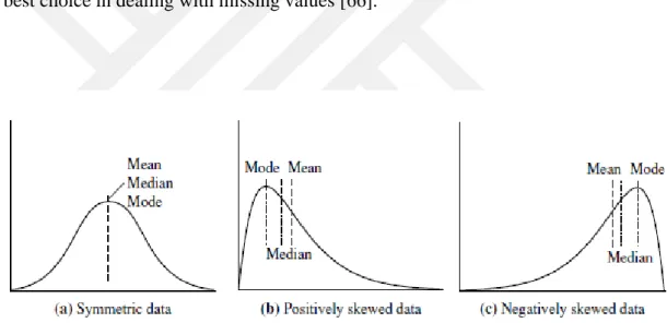
 Replace the missing value with Measures of Central Tendency: The most commonly used measures of central tendencies are the mean, median, and mode. Missing values for a given attribute are replaced by mean, median, or mode For normal data distributions, especially for symmetric data, mean can be used. But, for skewed data distribution, the median can be used.

 Replace the missing values with the most probable value: This may be determined with imputed values based on the other characteristics of the record. The question “What would be the most likely value for this missing value, given all the other attributes for a particular record?” should be answered. [66, 67].

4.1.1.2 Handling Noisy Data

When we say noisy , it refers to the change of a value, the addition of meaningless data or out of range values like a person filling out the numeric value -679 in the salary field or some negative four-digit random number in the age field. Noise is one of the random problems which is involved in measurement error. The process of removing noise from a dataset is termed as data smoothing. The following techniques can be used for noise reduction and data smoothing:

 Binning: It is a technique where the data is sorted and then partitioned into equal frequency bins. Then the noisy data may either be replaced with the bin mean bin median, or the bin boundary.

 Regression: Regression is used to find a mathematical equation to fit the data which helps to smooth out the noise [66].

(45)

28

4.1.1.3 Outliers Detection and Treatment

In Data Science, an outlier is simply an extreme value or data objects that have different characteristics from most of the other data objects in the dataset [69]. Causes of outlier may be due to measurement errors, incorrect data entry, or incorrect selection of a sample [67]. Figure 4.1 below provides a visual understanding of Outliers. According to Figure 4.1, the objects in region R can be identified as an outlier. Because, the other group of objects in the dataset is close to each other, falls into the same cluster, and follow the same distribution [66].

If there are outliers in the dataset, they can drastically change the results of the data analysis and give unreliable results. For example, they can increase the variance, decrease normality, and reduces the reliability of the tests [13, 70].

Figure 4.1: The objects in region R are outliers.

4.1.1.3.1 Outlier Detection

Outlier detection is the most important process of finding anomalies. It is used in many

applications such as fraud detection, or image processing. There are two outlier detection methods which are called univariate and multivariate. While the univariate method detects outliers on one variable, on the other hand, the multivariate method detects unusual combinations on all the variables.

In our analyses, we will be concerned with The Box Plot Rule[71] for outlier detection in univariate numerical data. It is a graphical tool used to construct a boxplot for more or less unimodal and symmetrically distributed data and to display a dataset based on

(46)

29

the five-number summary, such as the minimum, first quartile, median, third quartile, and maximum. In this method, the interquartile range (IQR) is used to find outliers and to filter out very large or small numbers. To create a boxplot as in Figure 4.2, the rules of the method are as: Firstly order the data from smallest to largest. Secondly, find the median, the first quartile(Q1), the third quartile(Q3), min, and max of the data. Then calculate the IQR which is the difference between the first and third quartile values. (Q3 - Q1). Next, calculate the lower fence, 1.5 X IQR. Q3 - [(IQR) x 1.5], and calculate the upper fence, 1.5 X IQR. Q3 + [(IQR) x 1.5]. Then, draw and label the axes of the graph and a box from Q1 to Q3 with a vertical line through the median. Finally, draw a whisker

from Q1 to the min and from Q3 to the max.

As a result, an outlier is any value that lies more than the upper fence or below the lower fence. Outliers lie outside the fences, that is, if a data point is below Q1 –

1.5×IQR or above Q3 + 1.5×IQR [72]. If we consider "extreme values", they are the

values lies between Min and Q1 – 3×IQR and Max and Q3 + 3×IQR. The outliers are

marked with asterisks(*) and extreme values are X [73].

Finally, it is assumed that values are normally clustered around some central value. The IQR demonstrates how the middle values spread out and how too far some of the other values from the central value are. These "too far" points are called "outliers" because they "lie outside" the range in which we expect them [73].

(47)

30

Additionally, histograms can also be used as a graphical method to identify outliers for numeric variables.

4.1.1.3.2 Removing Outliers

There are lots of strategies for dealing with deal with outliers. They are similar to the methods of missing values. In this research, the strategy of how to remove and when to replace outliers depends on the distribution of the data. Most of the data in applications are not symmetric, that is, they are either positively skewed or negatively skewed shown in Figure 4.3. Therefore, if we have approximately normal (symmetrical) distributions for continuous data, where all observations are nicely clustered around the mean which is a good option. However, for skewed distributions shown in Figure 4.3, the median is the best choice in dealing with missing values [66].

Figure 4.3: Mean, median, and mode of symmetric versus positively and negatively