1
Carbon emissions effect of energy transition and globalization: Inference from
the low, lower middle, upper middle and high-income economies
Andrew Adewale ALOLA 1, 2,
*
1 Department of Economics and Finance
Istanbul Gelisim University, Istanbul, Turkey
*Email: [email protected]
2 Department of Financial Technologies,
South Ural State University, Chelyabinsk, Russia
Udi JOSHUA
33 Department of Economic,
Federal University Lokoja, P.M.B 1154 Lokoja, Kogi state Nigeria.
Email –
[email protected]
Abstract
The importance of income to environmental sustainability especially in the perspective of economic development has been rigorously examined in recent times. To further deepened the environmental sustainability narrative, the current study explore the cases of income-classified countries vis-à-vis the high income, low income, lower middle income, and the upper middle income countries and territories. As such, the current study examined the impact of renewable energy and fossil fuel energy consumption and globalization on CO2 emissions over the
period of 1970 to 2014 for the case of (1) the panel of income-classified countries and territories and (2) the time series of each of the income-classification. By employing the Pooled Mean Group of the Autoregressive Distributed Lag (ARDL) approach, the study found that fossil fuel consumption in the panel of examined income classification aggravates environmental hazards in
2
both the short-long run while the share of renewable energy usage improves the environmental quality only in the short-run. Like the renewable energy consumption, globalization exacts negative and positive impact in the short-run and long run respectively. From the second (time series) approach, the study found that fossil fuel energy worsen the environment in each of the fours income-categorized economies. Similarly, renewable energy usage exerts a significant and desirable impact on the environment in all but one (lower middle income) of the four income-categorized economies. However, globalization observably plays a significant and desirable role only in the lower middle-income economies. Hence, the study posits policy guide in the context of increased diversification of energy portfolio for each of the four income-categorized countries and territories especially the lower middle-income economies.
Keyword: environmental sustainability; renewables; fossil fuel; carbon emissions: income-categorized economies.
1. Introduction
The debate on the relationship between economic transformation and energy usage is inexhaustible because of the peculiarity of the sector in promoting the course of economic advancement. Achieving and sustaining economic expansion and development remains the age-long key goal of every economy. Nations at different stages source for resources couple with key factors that could serve as engine to achieving this yearning objective. However, it is almost impossible to transform any economy whether developing or the so-called developed ones without energy consumption incorporated in the growth equation. This is because energy is a key factor that engineer economic activities and importantly that of the productive sectors of the economy such as the industrial sector. Invariably, energy consumption itself is not without negative consequences despites it significant contribution to economic expansion. Environmental degradation is the direct product of primary economic activities such as the extraction of the natural resources, agricultural activities as well as secondary economic activities such as the productive activity of the industrial sector (Ozturk, 2010; Alola & Alola, 2018; Recep & Faik, 2018; Danish, & Wang, 2019; Zhu et al., 2019). Thus, there is a tradeoff between energy usage-driven economic expansion and environmental degradation. Either a country would choose to expand and risk environmental
3
degradation cause by carbon emission or remain static as an opportunity cost/alternative of energy usage.
Because there is economic intuition for adopting the opportunity cost of energy usage, thus it is correct to assume that all economies of the world are prompt to future environmental degradation resulting from carbon emission. Thus, the relationship between economic well-being and ecological purity must be balanced if a nation desired to achieve a healthy and sustainable economic performance that will transcend to the future generation. The economic transformation that took place globally in the late 1980s is believed to be responsible for a higher derived demand for energy usage and consequently causing carbon emissions (Shahbaz et al., 2015). Shahbaz et al (2015) further revealed that the world development indicator shows that the annual per capital gross domestic product accelerates from $3596.67 in 1986-1990 to $10159.36 in 2010-2011. This trend keeps increasing significantly annually. For instance, in 2014 the figure increases to $15,342.848 and in most recently 2018 it escalated to $17,948.304. This sharp increase in the per capital income in turn cause a commensurable derive demand for energy usage, as the demand for energy consumption shifted tremendously from 1496.09-1917.98 kg of oil equivalent per capital in the time range between late 1970s to 1980 and 2010 to 2011. For the year 2014 specifically, energy consumption increases from the previous years to 1,922.488 (WDI 2018). This drastic change in energy demand cause by initial economic transformation transcended to significant expansion in carbon emission from 4.20 metric tons in 1986-1990 to 4.89 metric tons in 2010-2011 and to 4.981 metric tons for 2014 in particular.
Moreover, evidence from previous studies such as Bekun et al (2019a, 2019b) and Saint et al (2019) are few of the several studies that have affirmed the economic-carbon emission nexus. For instance, the World Bank in 2013 reported that world trade as a percentage of GDP accounts for 60.14% which increased to 71.70% in 2017 while trade in service as a percentage of GDP represents 12.25% in 2013 which equally improves to 12.95% in 2017 (World Development Indicator, WDI, 2018). The report further states that the rate of growth of trade flows increase from 1.04% in 2013 to 1.50% in 2017 despite the negative growth rate recorded in 2015 (-6.46 %) and 2016 (-1.59%). Thus, it is believed that trade globalization is an agent of technology, knowledge and innovation transfer from one country to another that play critical role in promoting the course
4
of economic expansion and performance. Furthermore, globalization traditionally assist in the process of redistribution of the unevenly deposition of natural resources, essential products and other raw materials across the globe. This assertion is aligned with the work of (see Shahbaz et al., 2013; Saint Akadiri, Alola & Akadiri, 2019; Zafar et al., 2019).
By attempting to explore the above motivations, the current study is aimed at achieving the objective of further revealing the impact of renewable energy usage, fossil fuel energy, and globalization especially for the case of low-income countries and territories, high-income countries and territories, lower middle-income countries and territories, and upper middle-income countries and territories. Although Ozturk, Aslan and Kalyoncu (2010), Shahbaz et al (2015) and Azam and Khan (2016) are the two close studies that have explore some of the income-categorized countries (low income high income, lower middle income, and upper middle income countries and territories
1), the current study is designed to further close the research gap in the extant studies through a
novel approach. The novelty of the current study is in folds. Firstly, this study employs the four World Bank income classification data (income group aggregate) for the (31) low-income economies, (79) high-income economies, (47) lower middle-income economies, and the (60) upper middle-income economies of total 217 countries and territories (see the Appendix A). Secondly, both the panel model of the four categories of income economies and the time series of each of the four categories of income economies are employed in a novel approach. To the best of authors’ knowledge, the aforementioned approaches are employed for the first time for the case of the aforementioned income-categorized economies, thus the contribution of the current study is a significant one.
The other sections of the study are arranged as follows. In section two and three, the extant literature and data description with methodological approach are respectively presented. The
1 According to the World Bank, Low income countries are countries or territories with a GNI per capita, calculated using the World
Bank Atlas method, of $1,025 or less in 2018. Low middle-income countries are countries or territories with a GNI per capita between $1,026 and $3,995. High-income economies are those in which 2017 GNI per capita was $12,055 or more. The Upper-middle-income economies are those in which 2017 GNI per capita was between $3,896 and $12,055.
5
empirical findings are subsequently discussed in section four while the last section (5) presents the concluding remarks with relevant policy recommendations.
2. A brief literature review
It appeared on the logical surface that energy consumption would automatically induce carbon emission without subjecting it to empirical investigation. However, this is not accepted in the research world as empirical assertions are only made after empirical investigation. The quest to ascertain the relationship connecting energy usage carbon emission and economic expansion has produced several conflicting outcomes. Some of the previous studies lent their voices to the positive contribution of energy consumption to quality environment while others oppose it, stressing that energy usage contribute to the expansion of carbon emission in addition to it positive contribution to economic progress. Others see energy usage from the perspective of economic transformation and development. example, the study of Saint et al., (2019) which adopted the ARDL bound test approach for the South Africa economy revealed that energy usage contributes to the increase in carbon emission while reverse is the case with real income per capital both in the near and future distance. The causal test proves that only energy usage induces environmental improvement and the real income per capital. The overall result indicates that environmental poor quality is proportional to the level of energy consumption as against other assertions that linked energy utilization with the rate of economic expansion. Similarly, Sarkodie and Adams (2018) make use of the ARDL bound testing to cointegration to investigate a disaggregated energy usage for the South Africa economy. The revelation from the findings shows that fossil fuel is a good contributor to carbon emission expansion in South Africa whereas renewable energy consumption sponsors the reversal direction of carbon emission. However, at the aggregate level energy consumption and economic expansion add to poor quality of the environment.
Destek and Sarkodie (2019) found an inverse as well as a two-way link between the variable of interest. Bekun et al., (2019) carried out similar study for the 16-EU countries and found that renewable energy usage is key to improving environmental quality in the study area. The study observed that economic expansion is one of the causes of carbon emission in addition to the detrimental role of fossil fuel on environmental quality. According to Bekun et al., (2019) only energy usage induces the quality of environment. Using an ARDL bound test for South Africa,
6
their findings further revealed that energy expansion is responsible in part to the economic acceleration in South Africa. Not only that they went further to establish through their finding that economic growth rather decreases the course of carbon emission. The study of Emir and Bekun (2019) revealed the existence of co-movement between the variables of interest. Further outcome shows that a bidirectional link between energy intensity and economic acceleration couple with an inducement only from energy usage to economic expansion. The study of Ulucak and Bilgili (2018) confirmed the EKC hypothesis depicting an inverse relationship between economic growth and carbon emission. Other related studies that lent their support to the ongoing debate include (see Apergis & Payne 2010; Apergis, N., & Ozturk, 2015; Ozturk, 2015; Solarin, Al-Mulali & Ozturk, 2017; Akadiri et al., 2019; Alola et al., 2019b;Ike et al., 2020; Lasisi et al., 2020).
Furthermore, the submission from the study of Shahbaz et al (2013 a & b) maintain that energy consumption serves as a panacea for economic expansion. They see energy usage as a key determining factor in the quest to achieving a sustainable economic acceleration, thus contradicting the work of (Jinke et al. 2008). According to them, the demand for energy consumption is induce by acceleration in the level of economic expansion. By this, they mean that when an economy experiences a sharp growth, the demand for coal consumption particularly to aid in power generation will be natural. Supporting this view are the work of (see Zhang and Xu 2012). Some studies that support feedback relationship between coal consumption and economic expansion includes (see Lee and Chang 2005; Adedoyin et al., 2020). Few other studies remain neutral as regard the influence of energy on economic expansion. These include (Jinke et al., 2008 & 2009; Stern 1993; Lee &Chang 2005; Koçak et al., 2019).
On the other hand, the relationship between trade openness and carbon emission has received serious attention from scholars who as usual failed to agree. For instance, Zafar et al., (2019) investigate the said relation in the case of OECD countries and the result indicates that trade openness play a role in improving environmental quality of the study area by reducing carbon emission which aligned with the work of Shahbaz et al., (2012 & 2013). On the contrary, the work of (see Mahrina & Sari 2019; Bekun et al., 2020) submit that globalization is one of the causes of economic breakdown through the promotion of carbon emission. The work of Omri et al., (2015) found a two-way interaction connecting economic expansion and carbon emission and that only
7
trade openness drives carbon emission in the MENA economies. Shahzad et al., (2017) investigate this contention for the Pakistani economy by adopting the ARDL bound test approach. The result indicates an inverse relationship between energy usage and economic expansion that suggest that an increase in energy usage will reduce carbon emission and improve environmental quality. The result further prove that trade openness and financial improvement add to carbon emission expansion both in the near and future distances. The granger causality on the other hand revealed a one-way causal effect flowing only from trade openness, energy usage and financial development to carbon emission. Similarly, the study of Shahbaz et al., (2017) carry out a panel study and found that trade openness is detrimental to an open economy both at the global level as well as for the regional classification base on income. The study found a mutual interaction between trade openness and carbon emission at global scene while a one-way causal effect was discovered for the high and low-income economies. Bernard and Mandal (2016) found a remarkable result in their study. Their findings revealed that energy usage, CO2 emission, trade openness and population explosion pose serious damage to the eco-system of the study area.
3. Data description and methodology
3.1 Data description
This study uses both the time series and panel data that is balanced for the low income, high income, lower middle income, and the upper middle-income countries and territories (comprising of 217 economies, see the list in the appendix) over the experimental period of 1970 to 2014. The estimation adopts carbon dioxide (CO2) as environmental variable for the dependent variable in
the model. The independent variables that are utilized include the renewable energy consumption, globalization, and the fossil fuel energy usage. The above-mentioned data series (income group aggregate) were retrieved from the World Bank (2017) Development indicator. Considering that, the cases examined are income-categorized and because of the unavailability of data for the low-income countries, the Gross Domestic Product (GDP) has been excluded from the estimation model. Additionally, the data span has been restricted to 1970-2014 due to the limited time period availability for CO2 series. Further information about the employed data is outlined in the Table
8
In addition, the summary statistics of the investigated series is further estimated and presented in the lower part of Table 1. Accordingly, it is found that the high-income economies have the highest CO2 emission with a mean of 11841424 Kilotons (Kt) followed by the upper middle-income
economies with the mean of 8079644 Kt of CO2 emission. Although a record high of 16827139
Kt of CO2 emissions is recorded in the upper middle income economies as against13753428 Kt in
the high income economies, the minimum level of CO2 emissions in the high income economies is however higher (9411515 Kt) against 2760635Kt in the case of upper middle income economies. Similarly, the trend of variation in the other series also implies that the high-income economies consumed more renewable and fossil fuel energy as well as having higher globalization. Thus, the order of variation of the series is higher in the high-income countries followed by the upper middle-income countries, the lower middle-income countries, and the low-income economies as shown in Table 1. The evidence of correlation among the variables is also presented in Table 2.
9 Table 1: Indicators and Descriptive Statistics
High Income Descriptive statistics
Variable Mean Median Maximum Minimum Skewness Kurtosis Jarque-Bera
CO2 11841424 11726315 13753428 9411515 -0.089 1.715 3.154 global 62.153 59.399 72.732 52.964 0.365 1.603 4.654*** rene 10.286 12.239 13.245 2.994 -0.981 2.321 8.081* fossil 86.036 83.406 94.716 81.257 0.827 2.103 6.641** Low Income CO2 137779.7 136616.8 221304.6 53524.11 -0.063 1.920 2.216 global 33.432 31.230 47.103 24.313 0.546 2.039 3.936 rene 2. 437 2.420 3.072 1.800 0.085 1.829 2.624 fossil 37.778 37.327 46.305 20.258 -0.922 3.822 7.645**
Lower Middle Income
CO2 2044470 2002253 4184823 658521.8 0.554 2.343 3.113
global 40.508 37.220 54.580 30.253 0.457 1.718 4.645**
rene 2.932 3.262 3.623 1.421 -1.124 2.891 9.494*
fossil 52.175 60.778 66.138 30.829 -0.388 1.431 5.742***
Upper Middle Income
CO2 8079644 7516624 16827139 2760635 0.833 2.753 5.313***
global 47.178 42.897 62.098 36.546 0.554 1.789 5.053***
rene 3.369 3.483 5.278 1.438 -0.296 1.880 3.009
fossil 79.540 83.145 87.542 65.654 -0.508 1.960 3.967
Note: WDI represents world development indicator (https://data.worldbank.org/). The CO2, global, rene, and fossil are respectively the Carbon dioxide, globalization, renewable energy consumption, and fossil fuel energy consumption.
Variables Code Unit of measurement Source
Globalization GLOBAL constant 2010 $ USD WDI
Renewable Energy Consumption RENE % of total final energy WDI
Carbon dioxide emissions CO2 (Kt) WDI
10
Table 2: Correlation Matrix_______________________________________________________
______________________________________________________________________________
Note: (*) Significant at the 1%. The CO2, global, rene, and fossil are respectively the Carbon dioxide, globalization, renewable energy consumption, and fossil fuel energy consumption.
3.2 Model and Methodology
In the context of the current studies, several relevant and recent studies have assessed the nexus of emissions, energy consumption, globalization, with few prioritizing the examined case to reflect income categorization (Shahbaz, Solarin, & Ozturk, 2016; Ozturk & Solarin, 2016; Jebli, Youssef & Ozturk, 2016; Ozcan, Ulucak & Dogan, 2019; Saint Akadiri et al., 2020a;Saint Akadiri et al., 2020b Usman, Alola & Sarkodie, 2020). While the current study examined the impact of renewable and fossil fuel energy consumption by also incorporating globalization, it implements this for the case of low income, lower middle income, upper middle income, high-income countries and territories in both time series and panel studies. The models employed for the purpose are presented as: 2 = ( , , ) (1) 2 = + + + + (2a) 2 = + + + + (2b) In order to utilize data with consistent variance, the logarithmic values of the series are employed. From the equations 1 and 2 above, the denotes the constant term while the βi (i = 1, 2, and 3)
Variable
CO2 FOSSIL RENE GLOBAL
CO2 1
FOSSIL 0.890* 1
RENE 0.762* 0.571* 1
11
represents the slope coefficients and εit is the stochastic term. Specifically, i represents the (4) cross
sections; low income, lower middle income, upper middle income, and high income economies and t is the time period (1970-2014) in a panel estimation panel as presented in equation 2a as against the time series estimation presented in 2b.
3.3 Panel Pooled Mean Group (PMG) estimation
As a prerequisite for panel data analysis, the stationarity of the estimated series (CO2,
globalization, renewable and fossil fuel energy consumption) is ascertained. To accomplish this task, the study employs two panel unit root tests: the Levin, Lin and Chu (LLC) and Im, Pesaran and Shin (IPS) by Levin, Lin & Chu (2002) and Im, Pesaran & Shin (2003) respectively. The result of the unit root tests as indicated in Table 3 implies a mixed order, thus the presenting the appropriateness of the PMG Autoregressive Distributed Lag (ARDL) by Pesaran et al. (1999). Importantly, considering that the standard ARDL estimation models are unequipped for controlling for bias, a blend of PMG estimator by Pesaran et al. (1999) and ARDL model provides a remedy for such deficiency as against other dynamic panel data model such as the generalized method of moments (GMM). Thus, the employed PMG-ARDL pathway for (2a) is presented as:
Δ = ∅ + ∑ Δ ( ) + ∑ Δ ( )+ (3)
= ( )− (4) where lny is the logarithmic value of the regressand variable (LCO2), lnX denotes the logarithmic
values of the regressors (renewable energy consumption (rene), the fossil fuel consumption (fossil), and globalization (global)) with same number of slacks q across singular cross-sectional units i in time t, Δ denotes the difference operator, ϕ is the alteration or adjustment coefficient, θ implies the long term coefficient that yields β and ψ enhances the behaviour of the model after reaching convergence while ε is the error term.
To further examined the impart of renewable energy consumption the fossil fuel consumption and globalization in the category of income-categorized countries, the time series approach is employed for each of the categories (say the low income, lower middle income, upper middle income, and high income countries and territories) In this case, the appropriateness of the ARDL-bound testing approach by Pesaran, Shin & Smith (2001) is maximized. The ARDL is effective
12
at estimating either small or a large sample size dataset. Also, the ARDL especially in the current case is appropriate in examining the short-run and long-run relationships. Thus, the unrestricted Autoregressive Distributed Lag (ARDL) method is employed for the above equation (2b) but the step-by-step approach by Pesaran Shin & Smith (2001)2 is not provided here for lack of space
3.3 Panel Granger Causality test
The Dumitrescu and Hurlin (2012) (referred herewith as DH) Granger causality test for heterogeneous non-causality is considered an effective approach in this context. The DH Granger causality approach is deemed applicable when T is larger than N, and vice versa. The DH is built on a vector autoregressive model (VAR) that is considered robust even in the presence of cross-sectional dependency. In this estimation, the asymptotic and semi-asymptotic are the two distinct distributions that are present in the procedure. However, the asymptotic distribution is employed in this case since T is larger than N as against the semi-asymptotic distribution that is considered appropriate when N is larger than T. Thus, the linear model specification is presented as:
yit= gi(k ) k=1 K
å
yi ,t-k+ bi( k) k=1 Kå
xi ,t-k+ei ,t (5)where K represents the lag length,
g
i( )k is the autoregressive parameter, whileb
i( )k represents the regression coefficient which is allowed to vary within the groups. The causality test is normally distributed and allows for heterogeneity. However, the homogenous non-stationary hypothesis is employed to estimate causal nexus with heterogeneous models. Thus, the null and alternative hypotheses for homogenous non-stationary causality are specified as follows:0
:
i0
H
b
=
=
i1,...
N
1:
i0
H
b =
=
i1,...
N
10
ib
=
iN
1+
1,
N
1+
2,....
N
2 Pesaran, M. H., Shin, Y., & Smith, R. J. (2001). Bounds testing approaches to the analysis of level
13
where the unknown parameter is denoted by
N
1 , which satisfies the condition0 £ N
1/ N < 1
. Consequently, the ratio ofN N
1/
is expected to be less than 1. But, shouldN
1=
N
,it then presents that no causality across cross-sections, thus this translates to failure to reject the null of homogenous non-stationary causality. But,N =
10
implies a causal nexus in the macro panel approach.4. Result and discussion
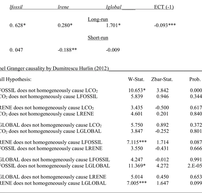
4.1 The panel short and long run impact
The results of the aforementioned ARDL Pooled Mean Group estimation and the panel Granger causality are presented in Table 4. Considering the significant elasticities of 0.047 and 0.626 in the short-run and long-run respectively, the ARDL Pooled Mean Group estimate presents that the consumption of fossil fuel energy is detrimental to the environment in the panel of low income, lower middle income, upper middle income, and high income countries and territories. This shows that there is no departure from the extant studies as regard the positive impact of fossil fuel consumption on CO2 emissions. Several studies especially that examined the impact of fossil fuel
consumption on the environment have equally reported that this type of energy portfolio worsen environmental quality (see Jebli, Youssef & Ozturk, 2016; Alola et al., 2019; Sharif et al., 2019 Adedoyin, Alola & Bekun, 2020; Asongu et al., 2020). For instance, the study of Nathaniel, Anyanwu and Shah (2020) supported that fossil fuel energy aggravates CO2 emission especially in the Middle East and North Africa (MENA) countries.
However, the impact of the renewable energy consumption on CO2 emissions in the short-run is
desirable. As such, a one percent increase in the renewable energy consumption is responsible for 18.8% decrease in the emission of CO2 emissions in the panel of income-categorized countries. In
previous studies such as Alola, Yalçiner and Alola (2019) for the case of Coastline Mediterranean Countries (CMCs), Saint Akadiri, and Alola (2020) for the United States, the renewable energy consumption is observed to yield desirable environmental sustainability. Interestingly, the impact of the renewable energy consumption on CO2 emissions is observably undesirable in the long run
since it causes 28% increase in CO2 emissions. Although, this observation is unexpected, previous
14
globalization on CO2 emissions is also observed to be negative and non-significant in the
short-run but the long-short-run impact is positive and significant. Accordingly, the study of Saint Akadiri, Alola and Akadiri (2019) equally implied that the impact of globalization on CO2 emissions
especially in the case of Turkey is negative but non-significant.
Table 4: Dynamic ARDL estimate_________________________________________________
lfossil lrene lglobal _____ ECT (-1)
Long-run
β 0. 628* 0.280* 1.701* -0.093***
Short-run
β 0. 047 -0.188** -0.009
Panel Granger causality by Dumitrescu Hurlin (2012)___________________________________
Null Hypothesis: W-Stat. Zbar-Stat. Prob.
LFOSSIL does not homogeneously cause LCO2 10.653* 3.842 0.000
LCO2 does not homogeneously cause LFOSSIL 5.839 0.946 0.344
LRENE does not homogeneously cause LCO2 3.435 -0.500 0.617
LCO2 does not homogeneously cause LRENE 4.601 0.201 0.840
LGLOBAL does not homogeneously cause LCO2 5.750 0.892 0.372
LCO2 does not homogeneously cause LGLOBAL 3.847 -0.252 0.801
LRENE does not homogeneously cause LFOSSIL 7.115*** 1.714 0.087
LFOSSIL does not homogeneously cause LRENE 3.550 -0.431 0.666
LGLOBAL does not homogeneously cause LFOSSIL 4.247 -0.012 0.991
LFOSSIL does not homogeneously cause LGLOBAL 11.369* 4.272 2.E-05
LGLOBAL does not homogeneously cause LRENE 5.014 0.450 0.653
LRENE does not homogeneously cause LGLOBAL 7.005*** 1.647 0.099
Note: (***) Significant at the 10%; (*) Significant at the 1%. The lCO2, lglobal, lrene, and lfossil are respectively the logarithmic of carbon dioxide, globalization, renewable energy consumption, and fossil fuel energy consumption.
4.2 Additional results
4.2.1 The panel Granger causality
By employing the Panel Granger causality by Dumitrescu Hurlin (2012), the causal relationship among the examined variables are presented in Table 4 above. Accordingly, there is a statistical
15
significant evidence of Granger causality from fossil fuel consumption to CO2 emissions. This
translates that the historical information of fossil fuel consumption is good enough to explain the present dynamics of the emission of CO2 in the panel countries. Similarly, there is a significant
evidence of Granger causality from renewable energy consumption to both the fossil fuel energy consumption and globalization. In addition, the statistical evidence of Granger causality from the fossil fuel energy consumption to globalization is also significant.
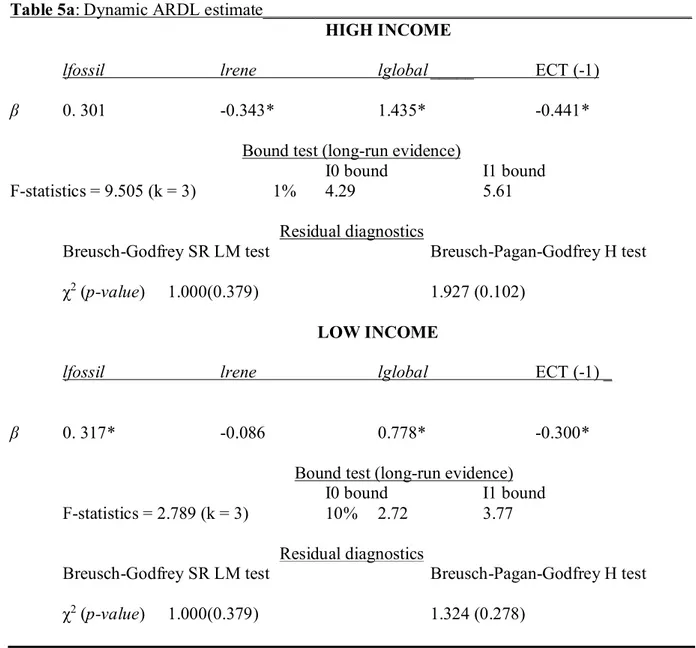
Table 5a: Dynamic ARDL estimate_________________________________________________ HIGH INCOME
lfossil lrene lglobal _____ ECT (-1)
β 0. 301 -0.343* 1.435* -0.441*
Bound test (long-run evidence)
I0 bound I1 bound
F-statistics = 9.505 (k = 3) 1% 4.29 5.61
Residual diagnostics
Breusch-Godfrey SR LM test Breusch-Pagan-Godfrey H test
χ2 (p-value) 1.000(0.379) 1.927 (0.102)
LOW INCOME
lfossil lrene lglobal ECT (-1) _
β 0. 317* -0.086 0.778* -0.300*
Bound test (long-run evidence)
I0 bound I1 bound
F-statistics = 2.789 (k = 3) 10% 2.72 3.77
Residual diagnostics
Breusch-Godfrey SR LM test Breusch-Pagan-Godfrey H test
χ2 (p-value) 1.000(0.379) 1.324 (0.278)
Note: Autoregressive Distributed Lad (ARDL) model employed models for the High income and Low Income are respectively (2,
1, 0, 1) and (1, 0, 0, 0). The β is the coefficient of the regressors, p-value is the probability value and ECT is the Error Correction Term also known as the adjustment parameter. The I0 and I1 are lower and upper bound of the bound test respectively, χ2 is the Chi-square, SR LM is Serial correlation Lagrange Multiplier and H is Heteroscedasticity. Also,
(), * and ** are the p-values, 1% significant level and 5% significant level respectively. The lCO2, lglobal, lrene, and lfossil are respectively the logarithmic of carbon dioxide, globalization, renewable energy consumption, and fossil fuel energy consumption.
16
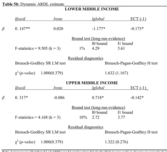
Table 5b: Dynamic ARDL estimate_________________________________________________ LOWER MIDDLE INCOME
lfossil lrene lglobal ECT (-1)
β 0. 147** 0.020 -1.177* -0.173*
Bound test (long-run evidence) I0 bound I1 bound
F-statistics = 9.505 (k = 3) 1% 4.29 5.61
Residual diagnostics
Breusch-Godfrey SR LM test Breusch-Pagan-Godfrey H test
χ2 (p-value) 1.000(0.379) 1.632 (1.167)
UPPER MIDDLE INCOME
lfossil lrene lglobal ECT (-1)_
β 0. 317* -0.086 0.718* -0.142*
Bound test (long-run evidence) I0 bound I1 bound
F-statistics = 4.168 (k = 3) 10% 2.72 3.77
Residual diagnostics
Breusch-Godfrey SR LM test Breusch-Pagan-Godfrey H test
χ2 (p-value) 1.000(0.379) 1.322 (0.276)
Note: Autoregressive Distributed Lad (ARDL) model employed models for the High income and Low Income are respectively (2,
1, 0, 1) and (1, 0, 0, 0). The β is the coefficient of the regressors, p-value is the probability value and ECT is the Error Correction Term also known as the adjustment parameter. The I0 and I1 are lower and upper bound of the bound test respectively, χ2 is the
Chi-square, SR LM is Serial correlation Lagrange Multiplier and H is Heteroscedasticity. Also, (), * and ** are the p-values, 1% significant level and 5% significant level respectively. The lCO2, lglobal, lrene, and lfossil are respectively the logarithmic of carbon dioxide, globalization, renewable energy consumption, and fossil fuel energy consumption.
4.2.2 Time series estimate results
Additionally, the result of the separate estimation (time series) ARDL bound test for each of the income categories especially in the short-run are presented in Tables 5a and 5b. With the elasticities of 0.301, 0.307, 0.147, and 0. 317 for the high-income economies, low-income economies, lower middle-income economies, and upper middle-income economies, it indicates that the consumption of fossil fuel energy hinders environmental sustainability of the examined
17
regions. In addition, with the exemption of the lower middle-income countries (elasticity is 0.020), the renewable energy consumption in the regions is statistically believed to aid the improvement of environmental quality. The reason for the unexpected result of CO2-reneeable energy
consumption nexus could be linked to the high composite of lower renewable sources in the renewable energy portfolio of the lower middle-income countries. On the other hand, globalization in the high-income countries, low-income countries, and the upper middle-income economies (with 1.435, 0.778, and 0.718 as respective elasticities) aggravates environmental hazards while the impact of globalization tends to mitigate carbon emissions in the lower middle-income countries and territories.
4.3 The diagnostic results
Adding to the aforementioned evidence, the F-statistics for each of the categorized income countries is greater the I0 bound limit (see Tables 5a and 5b). Also, the serial correlation test (p-value is 0.379) and the heteroscedasticity test (p-(p-value is 0.276) by Breusch-Godfrey Serial correlation Lagrange Multiplier (SR LM) test and Breusch-Pagan-Godfrey heteroscedasticity (H) test respectively provides statistical evidence of no serial correlation and heteroscedasticity problem. Lastly, the stability of the estimation (from model 2a) for each of the income-categorized countries is further affirmed by the Cumulative sum (CUSUM) (a) and CUSUM square test (b) in Figures 1, 2, 3, and 4.
18 -20 -15 -10 -5 0 5 10 15 20 15 20 25 30 35 40 45 CUSUM 5% Significance (a) -0.4 -0.2 0.0 0.2 0.4 0.6 0.8 1.0 1.2 1.4 15 20 25 30 35 40 45
CUSUM of Squares 5% Significance
(b)
Figure 1: The CUSUM (a) and CUSUM of Squares (b) residual diagnostic test for High Income countries and territories.
-20 -15 -10 -5 0 5 10 15 20 10 15 20 25 30 35 40 45 CUSUM 5% Significance (a) -0.4 -0.2 0.0 0.2 0.4 0.6 0.8 1.0 1.2 1.4 10 15 20 25 30 35 40 45
CUSUM of Squares 5% Significance
(b)
Figure 2: The CUSUM (a) and CUSUM of Squares (b) residual diagnostic test for Low Income countries and territories.
19 -20 -15 -10 -5 0 5 10 15 20 10 15 20 25 30 35 40 45 CUSUM 5% Significance (a) -0.4 -0.2 0.0 0.2 0.4 0.6 0.8 1.0 1.2 1.4 10 15 20 25 30 35 40 45
CUSUM of Squares 5% Significance
(b)
Figure 3: The CUSUM (a) and CUSUM of Squares (b) residual diagnostic test for Lower Middle Income countries and territories.
-20 -15 -10 -5 0 5 10 15 20 10 15 20 25 30 35 40 45 CUSUM 5% Significance (a) -0.4 -0.2 0.0 0.2 0.4 0.6 0.8 1.0 1.2 1.4 10 15 20 25 30 35 40 45
CUSUM of Squares 5% Significance
(b)
Figure 4: The CUSUM (a) and CUSUM of Squares (b) residual diagnostic test for Upper Middle Income countries and territories.
20
5. Conclusion and policy recommendation
As the concern of environmental sustainability has increasingly been examined within several context, studies have continued to reveal the determinants of environmental degradation especially for varying case studies. In the context of the current study, the impact of renewable energy consumption, the fossil fuel energy usage, and globalization on CO2 emissions is examined for (1)
the panel of income-categorized countries and (2) each of the income categories (the low income, high income, lower middle income, and upper middle-income economies). For the first approach, fossil fuel is responsible for increased carbon emissions in the panel countries and territories classification in both the short and long run. While both the renewable energy usage and globalization are responsible for the improvement of the quality of environmental both in the short-run, the impacts cause more environmental degradation in the long run. In the second approach, fossil fuel energy usage is responsible for increased carbon emissions in each of the income-classified country. In addition, the impact of renewable energy usage on CO2 emissions is
significant and negative in all the income-classified country except the lower middle-income economies. However, the environmental effect of globalization is significant but hazardous in all the income-classified country except for the lower middle-income countries. Thus, the study presents valuable policy implication for the high income, low income, lower middle income, and the upper middle-income countries.
5.1 Policy Recommendation
Considering that the study posits that fossil fuel energy contributes to enormous environmental damage as seen in the two estimation approaches, the countries and territories included in the income classifications should further adopts environmental-friendly energy portfolio. Importantly, the lower middle-income countries will need to adopt the policy that encourage more advancement/innovation of renewable energy sources. The aim of this policy mechanism is to increase the share of renewable energy source in the energy portfolio of the lower middle-income countries. Therefore, more interventions from the intergovernmental agencies in term of policy adoptions and provision of financial instrument could further guide most of the countries in the income-classified regions toward meeting their national sustainable developments targets.
21
References
Adedoyin, F. F., Alola, A. A., & Bekun, F. V. (2020). An assessment of environmental sustainability corridor: The role of economic expansion and research and development in EU countries. Science of The Total Environment, 136726.
Adedoyin, F. F., Gumede, M. I., Bekun, F. V., Etokakpan, M. U., & Balsalobre-Lorente, D. (2020). Modelling coal rent, economic growth and CO2 emissions: Does regulatory quality matter in BRICS economies?. Science of the Total Environment, 710, 136284.
Akadiri, S. S., Bekun, F. V., Taheri, E., & Akadiri, A. C. (2019). Carbon emissions, energy consumption and economic growth: a causality evidence. International Journal of Energy Technology and Policy, 15(2-3), 320-336.
Alola, A. A., & Alola, U. V. (2018). Agricultural land usage and tourism impact on renewable energy consumption among Coastline Mediterranean Countries. Energy & Environment, 29(8), 1438-1454.
Alola, A. A. (2019a). The trilemma of trade, monetary and immigration policies in the United States: Accounting for environmental sustainability. Science of The Total Environment, 658, 260-267.
Alola, A. A. (2019a). Carbon emissions and the trilemma of trade policy, migration policy and health care in the US. Carbon Management, 10(2), 209-218.
Alola, A. A., Saint Akadiri, S., Akadiri, A. C., Alola, U. V., & Fatigun, A. S. (2019a). Cooling and heating degree-days in the US: The role of macroeconomic variables and its impact on environmental sustainability. Science of The Total Environment, 695, 133832.
Alola, A. A., Yalçiner, K., & Alola, U. V. (2019). Renewables, food (in) security, and inflation regimes in the coastline Mediterranean countries (CMCs): the environmental pros and cons. Environmental Science and Pollution Research, 26(33), 34448-34458.
Alola, A. A., Yalçiner, K., Alola, U. V., & Saint Akadiri, S. (2019b). The role of renewable energy, immigration and real income in environmental sustainability target. Evidence from Europe largest states. Science of The Total Environment, 674, 307-315.
Apergis, N., & Payne, J. E. (2010). Coal consumption and economic growth: Evidence from a panel of OECD countries. Energy Policy, 38(3), 1353-1359.
Apergis, N., & Ozturk, I. (2015). Testing environmental Kuznets curve hypothesis in Asian countries. Ecological Indicators, 52, 16-22.
22
Asongu, S. A., Agboola, M. O., Alola, A. A., & Bekun, F. V. (2020). The criticality of growth, urbanization, electricity and fossil fuel consumption to environment sustainability in Africa. Science of The Total Environment, 136376.
Azam, M., & Khan, A. Q. (2016). Testing the Environmental Kuznets Curve hypothesis: A comparative empirical study for low, lower middle, upper middle and high income countries. Renewable and Sustainable Energy Reviews, 63, 556-567.
Bekun, F. V., Alola, A. A., & Sarkodie, S. A. (2019a). Toward a sustainable environment: Nexus between CO2 emissions, resource rent, renewable and nonrenewable energy in 16-EU countries. Science of the Total Environment, 657, 1023-1029.
Bekun, F. V., Emir, F., & Sarkodie, S. A. (2019b). Another look at the relationship between energy consumption, carbon dioxide emissions, and economic growth in South Africa. Science of the Total Environment, 655, 759-765.
Bekun, F. V., Yalçiner, K., Etokakpan, M. U., & Alola, A. A. (2020). Renewed evidence of environmental sustainability from globalization and energy consumption over economic growth in China. Environmental Science and Pollution Research, 1-15.
Danish, & Wang, Z. (2019). Investigation of the ecological footprint's driving factors: What we learn from the experience of emerging economies. Sustainable Cities and Society, 49. Destek, M. A., & Sarkodie, S. A. (2019). Investigation of environmental Kuznets curve for
ecological footprint: the role of energy and financial development. Science of the Total Environment, 650, 2483-2489.
Dumitrescu, E. I., & Hurlin, C. (2012). Testing for Granger non-causality in heterogeneous panels. Economic modelling, 29(4), 1450-1460.
Emir, F., & Bekun, F. V. (2019). Energy intensity, carbon emissions, renewable energy, and economic growth nexus: new insights from Romania. Energy & Environment, 30(3), 427-443.
Energy Information Administration (EIA), 2010. Country Analysis Brief South Africa. Retrieved 2018, from South Africa Energy Data, Statistics and Analysis - Oil, Gas, Electricity, Coal: https://www.eia.gov/beta/international/analysis_includes/countries_long/south_africa/arc hive/pdf/south_africa_2010.pdf.
23
Ike, G. N., Usman, O., Alola, A. A., & Sarkodie, S. A. (2020). Environmental quality effects of income, energy prices and trade: The role of renewable energy consumption in G-7 countries. Science of The Total Environment, 137813.
Im, K. S., Pesaran, M. H., & Shin, Y. (2003). Testing for unit roots in heterogeneous panels. Journal of econometrics, 115(1), 53-74.
Jebli, M. B., Youssef, S. B., & Ozturk, I. (2016). Testing environmental Kuznets curve hypothesis: The role of renewable and non-renewable energy consumption and trade in OECD countries. Ecological Indicators, 60, 824-831.
Jinke, L., Hualing, S., & Dianming, G. (2008). Causality relationship between coal consumption and GDP: difference of major OECD and non-OECD countries. Applied Energy, 85(6), 421-429.
Koçak, E., Ulucak, R., Dedeoğlu, M., & Ulucak, Z. Ş. (2019). Is there a trade-off between sustainable society targets in Sub-Saharan Africa?. Sustainable Cities and Society, 51, 101705.
Lasisi, T. T., Alola, A. A., Eluwole, K. K., Ozturen, A., & Alola, U. V. (2020). The environmental sustainability effects of income, labour force, and tourism development in OECD countries. Environmental Science and Pollution Research, 1-12.
Lee, C. C., & Chang, C. P. (2005). Structural breaks, energy consumption, and economic growth revisited evidence from Taiwan. Energy Economics, 27(6), 857-872.
Levin, A., Lin, C. F., & Chu, C. S. J. (2002). Unit root tests in panel data: asymptotic and finite-sample properties. Journal of econometrics, 108(1), 1-24.
Nathaniel, S., Anyanwu, O., & Shah, M. (2020). Renewable energy, urbanization, and ecological footprint in the Middle East and North Africa region. Environmental Science and Pollution Research, 1-13.
Ozcan, B., Ulucak, R., & Dogan, E. (2019). Analyzing long lasting effects of environmental policies: Evidence from low, middle and high-income economies. Sustainable Cities and Society, 44, 130-143.
Ozturk, I. (2010). A literature survey on energy–growth nexus. Energy policy, 38(1), 340-349. Ozturk, I. (2015). Sustainability in the food-energy-water nexus: Evidence from BRICS (Brazil,
24
Ozturk, I., Aslan, A., & Kalyoncu, H. (2010). Energy consumption and economic growth relationship: Evidence from panel data for low and middle-income countries. Energy Policy, 38(8), 4422-4428.
Pesaran, M. H., Shin, Y., & Smith, R. P. (1999). Pooled mean group estimation of dynamic heterogeneous panels. Journal of the American statistical association, 94(446), 621-634. Pesaran, M. H., Shin, Y., & Smith, R. J. (2001). Bounds testing approaches to the analysis of level
relationships. Journal of applied econometrics, 16(3), 289-326.
Saint Akadiri, S., & Alola, A. A. (2020). The role of partisan conflict in environmental sustainability targets of the United States. Environmental Science and Pollution Research, 1-10.
Saint Akadiri, S., Alola, A. A., & Akadiri, A. C. (2019). The role of globalization, real income, tourism in environmental sustainability target. Evidence from Turkey. Science of the total environment, 687, 423-432.
Saint Akadiri, S., Bekun, F. V., & Sarkodie, S. A. (2019). Contemporaneous interaction between energy consumption, economic growth and environmental sustainability in South Africa: What drives what? Science of the Total Environment, 686, 468-475.
Saint Akadiri, S., Alola, A. A., Bekun, F. V., & Etokakpan, M. U. (2020a). Does electricity consumption and globalization increase pollutant emissions? Implications for environmental sustainability target for China. Environmental Science and Pollution Research.
Saint Akadiri, S., Alola, A. A., Olasehinde-Williams, G., & Etokakpan, M. U. (2020b). The role of electricity consumption, globalization and economic growth in carbon dioxide emissions and its implications for environmental sustainability targets. Science of The Total Environment, 708, 134653.
Sarkodie, S. A., & Adams, S. (2018). Renewable energy, nuclear energy, and environmental pollution: accounting for political institutional quality in South Africa. Science of the total environment, 643, 1590-1601.
Shahbaz, M., Khan, S., & Tahir, M. I. (2013). The dynamic links between energy consumption, economic growth, financial development and trade in China: fresh evidence from multivariate framework analysis. Energy economics, 40, 8-21
25
Shahbaz, M., Tiwari, A. K., & Nasir, M. (2013). The effects of financial development, economic growth, coal consumption and trade openness on CO2 emissions in South Africa. Energy Policy, 61, 1452-1459.
Shahbaz, M., Nasreen, S., Abbas, F., & Anis, O. (2015). Does foreign direct investment impede environmental quality in high-, middle-, and low-income countries?. Energy Economics, 51, 275-287.
Shahbaz, M., Solarin, S. A., & Ozturk, I. (2016). Environmental Kuznets curve hypothesis and the role of globalization in selected African countries. Ecological Indicators, 67, 623-636. Sharif, A., Raza, S. A., Ozturk, I., & Afshan, S. (2019). The dynamic relationship of renewable
and nonrenewable energy consumption with carbon emission: A global study with the application of heterogeneous panel estimations. Renewable Energy, 133, 685-691.
Solarin, S. A., Al-Mulali, U., & Ozturk, I. (2017). Validating the environmental Kuznets curve hypothesis in India and China: The role of hydroelectricity consumption. Renewable and Sustainable Energy Reviews, 80, 1578-1587.
Stern, D. I. (1993). Energy and economic growth in the USA: a multivariate approach. Energy economics, 15(2), 137-150.
Ulucak, R., & Bilgili, F. (2018). A reinvestigation of EKC model by ecological footprint measurement for high, middle and low income countries. Journal of cleaner production, 188, 144-157.
Usman, O., Alola, A. A., & Sarkodie, S. A. (2020). Assessment of the role of renewable energy consumption and trade policy on environmental degradation using innovation accounting: Evidence from the US. Renewable Energy.
World Bank, 2018. Development indicators. http://databank.worldbank.org, Accessed date: July 2019
World coal institute. Coal facts; (2005) available at https://www.worldcoal.org/ accessed July 2019
World Energy Council, 2016.World Energy Resources 2016. Retrieved fromhttps://www. worldenergy.org/data/resources/resource/coal/.
Zhang, C., & Xu, J. (2012). Retesting the causality between energy consumption and GDP in China: Evidence from sectoral and regional analyses using dynamic panel data. Energy Economics, 34(6), 1782-1789.
26
Zhu, L., Hao, Y., Lu, Z. N., Wu, H., & Ran, Q. (2019). Do economic activities cause air pollution? Evidence from China’s major cities. Sustainable Cities and Society, 49, 101593.
Appendix
A: List of the World Bank income classification of countries and territories.
Low Income (31 countries with a GNI per capita, calculated using the World Bank Atlas method,
of $1,025 or less in 2018).
AFGHANISTAN, BENIN, BURKINA FASO, BURUNDI, CENTRAL AFRICAN REPUBLIC, CHAD, DEMOCRATIC REPUBLIC OF CONGO, ERITREA, ETHIOPIA, GAMBIA, THE GUINEA, GUINEA-BISSAU, HAITI, KOREA DEMOCRATIC PEOPLE’S REPUBLIC, LIBERIA, MADAGASCAR, MALAWI, MALI, MOZAMBIQUE, NEPAL, NIGER, RWANDA, SIERRA LEONE, SOMALIA, SOUTH SUDAN, SYRIAN ARAB REPUBLIC, TAJIKISTAN, TANZANIA, TOGO, UGANDA, AND YEMEN REPUBLIC.
Lower middle Income (47 countries with a GNI per capita between $1,026 and $3,995).
ANGOLA, BANGLADESH, BHUTAN, BOLIVIA, CABO VERDE, CAMBODIA, CAMEROON, COMOROS, CONGO REPUBLIC, COTE D'IVOIRE, DJIBOUTI, EGYPT, ARAB REPUBLIC, EL SALVADOR, ESWATINI, GHANA, HONDURAS, INDIA, INDONESIA, KENYA, KIRIBATI, KYRGYZ REPUBLIC, LAO PDR, LESOTHO, MAURITANIA, MICRONESIA FEDERAL STS., MOLDOVA, MONGOLIA, MOROCCO, MYANMAR, NICARAGUA, NIGERIA, PAKISTAN, PAPUA NEW GUINEA, PHILIPPINES, SAO TOME AND PRINCIPE, SENEGAL, SOLOMON ISLANDS, SUDAN, TIMOR-LESTE, TUNISIA, UKRAINE, UZBEKISTAN, VANUATU, VIETNAM, WEST BANK AND GAZA, ZAMBIA, AND ZIMBABWE.
High Income (79 High-income economies are those in which 2017 GNI per capita was $12,055
27
ANDORRA, ANTIGUA AND BARBUDA, ARUBA, AUSTRALIA, AUSTRIA, BAHAMAS, THE BAHRAIN, BARBADOS, BELGIUM, BERMUDA, BRITISH VIRGIN ISLANDS, BRUNEI DARUSSALAM, CANADA, CAYMAN ISLANDS, CHANNEL ISLANDS, CHILE, CROATIA, CURACAO, CYPRUS, CZECH REPUBLIC, DENMARK, ESTONIA, FAROE ISLANDS, FINLAND, FRANCE, FRENCH POLYNESIA, GERMANY, GIBRALTAR, GREECE, GREENLAND, GUAM, HONG KONG SAR CHINA, HUNGARY, ICELAND, IRELAND, ISLE OF MAN, ISRAEL, ITALY, JAPAN, KOREA REPUBLIC, KUWAIT, LATVIA, LIECHTENSTEIN, LITHUANIA, LUXEMBOURG, MACAO SAR CHINA, MALTA, MONACO, NETHERLANDS, NEW CALEDONIA, NEW ZEALAND, NORTHERN MARIANA ISLANDS, NORWAY, OMAN, PALAU, PANAMA, POLAND, PORTUGAL, PUERTO RICO, QATAR, SAN MARINO, SAUDI ARABIA, SEYCHELLES, SINGAPORE, SINT MAARTEN (DUTCH PART), SLOVAK REPUBLIC, SLOVENIA, SPAIN, ST. KITTS AND NEVIS, ST. MARTIN (FRENCH PART), SWEDEN, SWITZERLAND, TRINIDAD AND TOBAGO, TURKS AND CAICOS ISLANDS, UNITED ARAB EMIRATESM UNITED KINGDOM, UNITED STATES, URUGUAY, AND VIRGIN ISLANDS (U.S.)
Upper middle Income (60 Upper-middle-income economies are those in which 2017 GNI per
capita was between $3,896 and $12,055).
ALBANIA, ALGERIA, AMERICAN SAMOA, ARGENTINA, ARMENIA, AZERBAIJAN, BELARUS, BELIZE, BOSNIA AND HERZEGOVINA, BOTSWANA, BRAZIL, BULGARIA, CHINA, COLOMBIA, COSTA RICA, CUBA, DOMINICA, DOMINICAN REPUBLIC,
ECUADOR, EQUATORIAL GUINEA, FIJI, GABON, GEORGIA, GRENADA,
GUATEMALA, GUYANA, IRAN ISLAMIC REPUBLIC, IRAQ, JAMAICA, JORDAN, KAZAKHSTAN, KOSOVO, LEBANON, LIBYA, MALAYSIA, MALDIVES, MARSHALL ISLANDS, MAURITIUS, MEXICO, MONTENEGRO, NAMIBIA, NAURU, NORTH MACEDONIA, PARAGUAY, PERU, ROMANIA, RUSSIAN FEDERATION, SAMOA, SERBIA, SOUTH AFRICA, SRI LANKA, ST. LUCIA, ST. VINCENT AND THE GRENADINES, SURINAME, THAILAND, TONGA, TURKEY, TURKMENISTAN, TUVALU, AND VENEZUELA RB.