Resonant harmonic response in tapping-mode atomic force microscopy

Resonant harmonic response in tapping-mode atomic force microscopy

Ozgur Sahin,*Calvin F. Quate, and Olav Solgaard

E. L. Ginzton Laboratory, Stanford University, Stanford, California 94305, USA Abdullah Atalar

Electrical and Electronics Engineering Department, Bilkent University, Bilkent, 06533 Ankara, Turkey 共Received 4 December 2003; published 28 April 2004兲

Higher harmonics in tapping-mode atomic force microscopy offers the potential for imaging and sensing material properties at the nanoscale. The signal level at a given harmonic of the fundamental mode can be enhanced if the cantilever is designed in such a way that the frequency of one of the higher harmonics of the fundamental mode共designated as the resonant harmonic兲 matches the resonant frequency of a higher-order flexural mode. Here we present an analytical approach that relates the amplitude and phase of the cantilever vibration at the frequency of the resonant harmonic to the elastic modulus of the sample. The resonant harmonic response is optimized for different samples with a proper design of the cantilever. It is found that resonant harmonics are sensitive to the stiffness of the material under investigation.

DOI: 10.1103/PhysRevB.69.165416 PACS number共s兲: 68.37.Ps, 07.79.Lh, 87.64.Dz

I. INTRODUCTION

The atomic force microscope1 共AFM兲 is primarily a tool for characterizing surface topography, but there is always a strong interest in using this technique to study the mechani-cal properties of samples at the nanosmechani-cale. A method for probing elastic and viscoelastic surface properties will en-hance our ability to characterize materials, map variations in chemical composition, and investigate the properties of nanostructures. The techniques for measuring these proper-ties include force modulation microscopy,2 the force curve method,3 nanoindentation,4 pulsed force mode,5 and ultra-sonic force microscopy.6 – 8 These techniques measure the elastic properties either directly by indenting the surface with a force applied to the tip or indirectly by monitoring the response of the cantilever with the tip in contact with the surface. The latter is more sensitive to the local stiffness of the samples,9–11 but sometimes results in damage. Probing the surface with the tapping mode for the AFM共Ref. 12兲 is a more gentle procedure that largely eliminates damage to the sample.

In tapping mode the cantilever is driven at the resonant frequency of the fundamental mode with the tip periodically tapping on the surface. A feedback loop is used to maintain the excursion of the oscillating tip at a constant level. The variations in both amplitude and phase of the feedback signal reveal the surface topography. Images obtained with the phase signal exhibit good contrast for different materials.13,14 Unfortunately, multiple sources of dissipation, such as capil-lary forces,15viscoelasticity of samples, and electronic dissi-pation, make it difficult to interpret the phase signal and relate it to material properties. Balantekin and Atalar16have suggested that the elastic and viscoelastic properties can be inferred from the amplitude and phase of the cantilever mo-tion if the mechanical parameters of the cantilevers are known. Their model is limited to hydrophobic surfaces since it does not account for the capillary forces between the tip and the sample. Stark et al. have shown that the phase signal is influenced by the topographical variations,17which makes

it difficult to interpret the image. Recently, Rodriguez and Garcia18 proposed excitation of the first modes of the canti-lever to create coupled anharmonic oscillators with high sen-sitivity to variations in the attractive component of the tip-sample forces that depend on the chemical composition of the sample.

There is a wealth of information in the harmonics gener-ated when the tip periodically taps on the sample surface.19–21 Heretofore, this information has been hidden beneath the noise floor because of the rapid decay of the amplitude of the harmonics.22 Here we show that a simple modification of the cantilever enhances the amplitude of a selected harmonic and increases the signal-to-noise ratio to a reasonable level. We have learned that the amplitude of the higher harmonics can be enhanced with specially microma-chined cantilevers altered in such a way that the third flex-ural mode is an exact integer multiple of the fundamental resonance frequency.23 Simulations show that under these conditions the selected harmonic is very sensitive to material properties.24Hereafter, we will designate the harmonics that match the frequency of a flexural mode as resonant har-monic. These special cantilevers enable a new imaging mode where we monitor the cantilever deflection at the harmonic corresponding to the third flexural mode. In this paper, we present a model for the response of a resonant harmonic in tapping-mode atomic force microscopy. We use this model to calculate the amplitude and phase of resonant harmonics for a variety of samples and demonstrate that the harmonics serve as a sensitive probe of material properties.

II. THEORY

In tapping mode, the cantilever is driven at the resonant frequency of the fundamental. When it is brought closer to the sample, the tip will periodically contact the sample. As the tip taps on the surface, the periodic impulse25will excite the flexural modes together with the higher harmonics. The amplitude of the harmonics is determined by a variety of parameters as outlined in a later section. Stark and Heckl26

have calculated the amplitudes of the higher harmonics by treating the tip-sample interaction as a linear spring and modeling the cantilever with a continuum mechanical sys-tem. In this paper we will follow the work of Sarid et al.27 and model the repulsive forces with the theory of Hertzian contacts and the attractive forces with the theory of Van der Waals interactions. We will use continuum mechanics to ana-lyze a cantilever that have been modified so that the fre-quency of one of the higher flexural models matches the frequency of a harmonic of the fundamental frequency.

A. Calculating the harmonics of tip-sample interaction forces Various aspects of the dynamics of tapping-mode atomic force microscopy共TM-AFM兲 have been studied in detail for real and model systems.28 –35Here we will calculate the time course of tip-sample interaction forces, and evaluate the har-monics with the Fourier transform.

We are able to use the harmonic approximation to calcu-late tip-sample interaction forces because the quality factor of the cantilevers is very high. Although tip-sample interac-tion contains several harmonics, it is mostly the fundamental harmonic at the driving frequency that affects the motion of the cantilever, because it is at the resonance frequency. Other harmonics act on the tip, but the frequency response of the cantilever at those frequencies is smaller共two to three orders of magnitude兲 than the response at the fundamental reso-nance frequency. Unfortunately, this approximation cannot be used for cantilevers immersed in liquids because the in-creased damping reduces the quality factor.

If we neglect the contribution of higher harmonics of the tip-sample interaction force on the cantilever motion, the problem is reduced to one of calculating the motion of a cantilever driven at its resonance frequency from both the base and tip. The driving force at the base will generate a free amplitude of A0. The force at the tip is unknown and we are faced with the task of finding the magnitude and phase

共relative to the phase of the cantilever motion兲 in terms of the

free vibration amplitude, set-point amplitude As, phase of

cantilever motion 共relative to the driving signal兲, and the spring constant and quality factor of the cantilever. If we set the phase of the cantilever oscillation to zero, the motion of the cantilever can be written as Asei␻t. We represent the

driving force and the fundamental harmonic of the tip-sample force as F_dei(␻t⫹␾) and F_ts1ei(␻t⫹␪), respectively,

FTei共␻t⫹␲/2兲⫽Fdei共␻t⫹␾兲⫹Fts1ei共␻t⫹␪兲. 共1兲 Here the␲/2 phase associated with the total force FTis due

to the resonance of the cantilever, since on resonance the oscillations of the cantilever follow the total force with a phase delay of␲/2. Balantekin and Atalar36used the phasor representation of Eq. 共1兲 and studied the dynamics of a vi-brating cantilever in noncontact. In Eq.共1兲, FTand Fdcan be

written in terms of the spring constant K1, quality factor Q1, free amplitude A0, and set-point amplitude As as follows:

Fd⫽K1A0/Q1, 共2兲 FT⫽K1As/Q1. 共3兲

Equation 共2兲 describes a freely vibrating cantilever at reso-nance. In Eq. 共3兲 we treat the cantilever as a linear system and the tip-sample force together with the driving force are the inputs to this system. So even though the tip-sample force is nonlinear, the total force and displacement of the cantilever satisfy the linear relation of Eq.共3兲. A similar ap-proach is used by Stark et al.,20 who modeled tip-sample forces as nonlinear feedback acting on the linear system of the cantilever. In Eq.共3兲, F_T represents the sum of the non-linear tip-sample forces and the driving force. Therefore, the output of the cantilever, which is the tip displacement, will satisfy the linear relation valid for a freely vibrating cantile-ver. In this approach, all the nonlinearity in the TM-AFM system is hidden in FT. By writing Eq.共3兲, we are not

ne-glecting the nonlinear contributions from the tip-sample in-teraction, however we are separating the linear and nonlinear parts of the mathematical problem to the solution.

When we substitute Eq. 共2兲 and Eq. 共3兲 into Eq. 共1兲 and equate the real and imaginary parts of Eq. 共1兲, we get the following relations: K1A0 Q1 cos␾⫹F_ts1cos␪⫽0, 共4兲 K1A0 Q1 sin␾⫹Fts1sin␪⫽ K1A1 Q1 . 共5兲

These equations relate the magnitude and phase of the fun-damental harmonic of fts to the known parameters of the tapping-mode operation. When we solve these equations for the magnitude Fts1 and phase␪, we get

Fts1⫽ K₁A₀ Q1

冋

1⫺2As A0 sin␾⫹As 2 A₀2

册

1/2 , 共6兲

␪⫽tan⫺1

冉

As⫺A0sin␾

A₀cos␾

冊

. 共7兲 These equations relate the magnitude and phase of the fun-damental harmonic force to the measurable parameters of the cantilever.

An interesting and useful parameter in TM-AFM is the tip-sample energy dissipation due to the nonconservative na-ture of the interaction forces. We would like to calculate tip-sample energy dissipation with the sample approach as we did for the calculation of the fundamental harmonic of the tip-sample forces. Energy dissipation per oscillation cycle can be calculated by integrating the instantaneous power共the product of tip velocity and tip-sample force兲 over one cycle as Edis⫽⫺

冕

2␲/␻ fts共t兲y共t兲dt⫽

冕

2␲/␻ As␻ftssin共␻t兲dt. 共8兲 Here y (t) is the first derivative of the position of the tip with respect to time. If y (t) is chosen as Ascos(␻t), then y (t) is

equal to ⫺As␻cos(␻t). fts is the tip-sample force in time domain. Note that no particular interaction model is assumed and this equation is valid for any fts. The only approxima-tion we make is the harmonic approximaapproxima-tion, i.e., we assume

a pure sinusoidal tip motion. Other than multiplicative terms, this integral is equivalent to the coefficient of sin(␻t) in Fou-rier series expansion of fts, which is equal to ⫺Fts1sin␪. Rewriting Eq. 共8兲 with this replacement, we get

Edis⫽⫺␲AsFts1sin␪. 共9兲 In this equation, Fts1 is given by Eq. 共6兲 and␪ is given by Eq.共7兲. Note that for a dissipative f_ts,sin(␪) is always nega-tive so that energy dissipation is a posinega-tive quantity. Inserting the values for Fts1 and␪gives the more familiar relation for the energy dissipation per oscillation cycle for a cantilever driven at resonance,13,14 Edis⫽ ␲K1As 2 Q1

冋

A0 As sin␾⫺1

册

. 共10兲

This relationship has been derived earlier by considering the energy loss of tip-sample interaction. That we now find the same expression based on considerations of the tip-sample forces is an indication that our assumptions and model are correct. It is important to note the relation between phase ␾ of the cantilever relative to the driving force and phase ␪of the tip-sample interaction forces relative to the cantilever motion. Equation共10兲 relates ␾to the energy dissipation at the tip-sample contact. Because A_s and A₀ are constants, we find in Eq.共7兲 that␪ is also a measure of energy dissipation in the tip-sample contact. In fact, a nonzero ␪means asym-metric tip-sample forces in approach and retraction of the tip, which in turn means that tip-sample forces are nonconserva-tive.

Equation 共6兲 shows that Fts1 depends on the mechanical properties of the cantilever and the motion of the cantilever. Other than ␾, these parameters are independent of the sur-face properties. Since␾depends on the energy dissipation in tip-sample contact 关see Eq. 共10兲兴, Fts1 also depends on tip-sample energy dissipation.

In order to calculate the time course of interaction forces for a sample with known material properties from Fts, we note that the time dependence of the tip-sample forces is determined by the maximum indentation depth共i.e., indenta-tion of the sample when the tip is at its lowest posiindenta-tion兲, which is equivalent to the minimum tip-sample separation in the attractive operation regime. There are two reasons for this. First, the cantilever motion remains nearly sinusoidal in typical tapping-mode operation when the cantilever has a high-quality factor, and second, the tip-sample force depends only on tip-sample separation and sample indentation. For a given depth of indentation, the time dependence of the tip-sample separation and tip-sample indentation is fully deter-mined. With this information, an interaction model can be used to calculate the tip-sample forces. The interaction model we used for the tip-sample forces assumes a Lennard-Jones type of distance dependence for the attractive forces, as shown below, fts共r兲⫽ HR 6␴2

冋

⫺

冉

␴ r

冊

2 ⫹₃₀1

冉

␴_r

冊

8

册

. 共11兲

Here r is the tip-sample separation, H is the Hamaker con-stant, R is the tip radius, and␴is the typical atomic distance for the tip and the surface. This force is attractive for tip-sample separations larger than r0⫽30⫺1/6␴. To account for energy dissipation in tip-sample interaction, we used two H values for the approach and retraction of the cantilever. This may not be the most realistic method for including the en-ergy dissipation. However, enen-ergy dissipation plays an im-portant role in the dynamics of tip motion as indicated by the hysteresis in adhesion forces that is observed in the tip-sample interaction. For small separations, the tip-sample is de-formed under the influence of repulsive forces. The sample indentation with a Hertzian contact is approximately

fts共d兲⫽

4 3E

冑

Rd

3/2_{, 共12兲}

where d is the deformation of the sample. The parameter E is the reduced elastic modulus of the tip and is given by

1 E⫽ 1⫺␯_t2 Et ⫹1⫺␯s 2 Es . 共13兲

Here Et,␯t and Es,␯s are the elastic modulus and Poisson’s

ratios of the tip and the sample, respectively. We use Eq.共11兲 for tip-sample separations larger than r0, where the force is attractive, and Eq. 共12兲 for the positive repulsive force.

The tip-sample interaction model assumes that tip-sample energy dissipation is due to the attractive forces regardless of sample indentation. This simplifies the calculation, which is justified by noting that most of the samples energy is dissi-pated by capillary forces and hysteresis in the Van der Waals attractive force. With viscoelastic samples the energy is dis-sipated when the tip indents the sample. If we assume con-stant dissipation of the tip-sample energy, the phase of the cantilever motion ␾is determined by Eq.共10兲. Equation 共6兲 determines the interaction force Fts1. Knowing Fts1, we can calculate the tip-sample forces for increasing depths of in-dentation starting at 0 and increasing until the interaction force has a fundamental harmonic equal to the predetermined value of Fts1. In the case of multiple solutions we pick the solution that belongs to the repulsive regime by looking at the sign of the average tip-sample force. The higher har-monic forces are calculated by taking the Fourier transform of the corresponding fts.

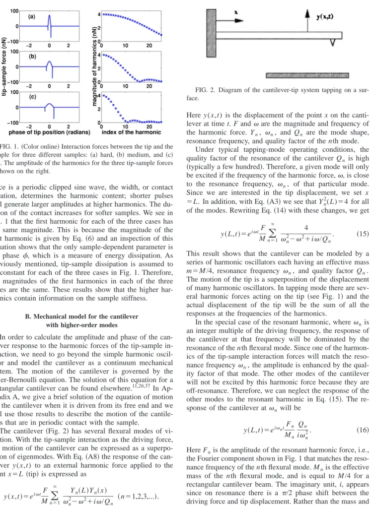
The tip-sample interactions for hard, medium, and soft samples are shown in Fig. 1. The Fourier components are calculated for a cantilever with spring constant K1⫽10, qual-ity factor Q1⫽100, free amplitude A0⫽100 nm, and set-point amplitude As⫽80 nm. The reduced Young’s modulus E for the three samples is chosen to obtain contact durations of 5%, 10%, and 15% of the period on the hard, medium, and soft samples, respectively. Attractive forces on all the samples are assumed to be equal for the same amount of energy dissipation at the contact. For the Hamaker constants we used Ha⫽10⫻10⫺20J for approach and Hr⫽30

⫻10⫺20_{J for retraction. The parameters R and␴are chosen}

to be 10 and 0.1 nm, respectively. These values result in an energy dissipation of approximately 30 eV per tap.

According to Fig. 1, harmonics above the fifth are depen-dent on the hardness of the sample. Since the tip-sample

force is a periodic clipped sine wave, the width, or contact duration, determines the harmonic content; shorter pulses will generate larger amplitudes at higher harmonics. The du-ration of the contact increases for softer samples. We see in Fig. 1 that the first harmonic for each of the three cases has the same magnitude. This is because the magnitude of the first harmonic is given by Eq. 共6兲 and an inspection of this equation shows that the only sample-dependent parameter is the phase ␾, which is a measure of energy dissipation. As previously mentioned, tip-sample dissipation is assumed to be constant for each of the three cases in Fig. 1. Therefore, the magnitudes of the first harmonics in each of the three cases are the same. These results show that the higher har-monics contain information on the sample stiffness.

B. Mechanical model for the cantilever with higher-order modes

In order to calculate the amplitude and phase of the can-tilever response to the harmonic forces of the tip-sample in-teraction, we need to go beyond the simple harmonic oscil-lator and model the cantilever as a continuum mechanical system. The motion of the cantilever is governed by the Euler-Bernoulli equation. The solution of this equation for a rectangular cantilever can be found elsewhere.11,26,37 In Ap-pendix A, we give a brief solution of the equation of motion for the cantilever when it is driven from its free end and we will use those results to describe the motion of the cantile-vers that are in periodic contact with the sample.

The cantilever 共Fig. 2兲 has several flexural modes of vi-bration. With the tip-sample interaction as the driving force, the motion of the cantilever can be expressed as a superpo-sition of eigenmodes. With Eq.共A8兲 the response of the can-tilever y (x,t) to an external harmonic force applied to the point x⫽L 共tip兲 is expressed as

y共x,t兲⫽ei␻tF Mn

兺

_⫽1 ⬁ Yn共L兲Yn共x兲 ␻n 2_⫺ ␻2_⫹i␻/Q n 共n⫽1,2,3,...兲. 共14兲

Here y (x,t) is the displacement of the point x on the canti-lever at time t. F and ␻are the magnitude and frequency of the harmonic force. Yn, ␻n, and Qn are the mode shape,

resonance frequency, and quality factor of the nth mode. Under typical tapping-mode operating conditions, the quality factor of the resonance of the cantilever Qn is high 共typically a few hundred兲. Therefore, a given mode will only

be excited if the frequency of the harmonic force,␻, is close to the resonance frequency, ␻n, of that particular mode.

Since we are interested in the tip displacement, we set x

⫽L. In addition, with Eq. 共A3兲 we see that Yn

2_{(L)⫽4 for all} of the modes. Rewriting Eq.共14兲 with these changes, we get

y共L,t兲⫽ei␻tF Mn

兺

⫽1 ⬁ ₄ ␻n 2_⫺ ␻2_⫹i␻/Q n . 共15兲

This result shows that the cantilever can be modeled by a series of harmonic oscillators each having an effective mass m⫽M/4, resonance frequency ␻n, and quality factor Qn.

The motion of the tip is a superposition of the displacement of many harmonic oscillators. In tapping mode there are sev-eral harmonic forces acting on the tip 共see Fig. 1兲 and the actual displacement of the tip will be the sum of all the responses at the frequencies of the harmonics.

In the special case of the resonant harmonic, where␻n is

an integer multiple of the driving frequency, the response of the cantilever at that frequency will be dominated by the resonance of the nth flexural mode. Since one of the harmon-ics of the tip-sample interaction forces will match the reso-nance frequency␻n, the amplitude is enhanced by the

qual-ity factor of that mode. The other modes of the cantilever will not be excited by this harmonic force because they are off-resonance. Therefore, we can neglect the response of the other modes to the resonant harmonic in Eq. 共15兲. The re-sponse of the cantilever at ␻_n will be

y共L,t兲⫽ei␻ntFn

Mn

Qn

i␻_n2. 共16兲 Here Fnis the amplitude of the resonant harmonic force, i.e.,

the Fourier component shown in Fig. 1 that matches the reso-nance frequency of the nth flexural mode. Mnis the effective

mass of the nth flexural mode, and is equal to M /4 for a rectangular cantilever beam. The imaginary unit, i, appears since on resonance there is a ␲/2 phase shift between the driving force and tip displacement. Rather than the mass and resonant frequency, we find it more convenient to work with

FIG. 1.共Color online兲 Interaction forces between the tip and the sample for three different samples: 共a兲 hard, 共b兲 medium, and 共c兲 soft. The amplitude of the harmonics for the three tip-sample forces is shown on the right.

FIG. 2. Diagram of the cantilever-tip system tapping on a sur-face.

the effective spring constants of the modes. Using the rela-tion␻2⫽k/m between mass, spring constant, and resonance frequency of a harmonic oscillator, we define an effective spring constant Kn⫽Mn␻n

2 _{for each flexural mode of the} cantilever. The effective masses of the modes of a rectangu-lar cantilever are the same and one can write

Kn K1 ⫽

冉

␻n ␻1

冊

2 . 共17兲

This equation relates the effective spring constant of a higher-order mode to the quantities ␻1, ␻n, and K1. This equation provides a rough estimate but it is sufficient for our discussion of the potential of resonant harmonics for study-ing material properties.

III. RESULTS AND DISCUSSION

Now we have a complete formulation required to calcu-late the resonant harmonic response in tapping mode. We first calculate the tip-sample interaction forces and its har-monic content as described in the previous section and then we calculate the displacement of the cantilever at the reso-nant harmonic using Eq. 共16兲. Using this methodology, we analyze the effects of the sample stiffness on the resonant harmonic. First, we calculate the resonant harmonic response as a function of reduced Young’s modulus E. Based on the results of these calculations, we discuss how the amplitude and phase response relate to sample stiffness. Second, we study the effects of cantilever spring constant and set-point amplitude on the resonant harmonic response. Finally, we consider the harmonic number that is to be enhanced by a flexural resonance. We show that appropriate selection of cantilever spring constant and harmonic number can enhance the resolution of resonant harmonic AFM.

For a given Young’s modulus we calculate the tip-sample interaction force fts as described in the theory section. The harmonic forces are calculated by taking its Fourier trans-form. Because f_ts is a periodic waveform, we can expand it into Fourier series as follows:

fts共t兲⫽

兺

k⫽0

⬁

ancos共k␻t兲⫹bnsin共k␻t兲 共k⫽0,1,2,...兲, 共18兲

where the frequency␻is the driving frequency. Coefficients akand bkare given as

ak⫽␻ ␲

冕

0 2␲/␻ ftscos共k␻t兲dt, 共19a兲 bk⫽␻ ␲

冕

0 2␲/␻ ftssin共k␻t兲dt. 共19b兲 The kth harmonic force can be written as

F_tskcos共k␻t⫹␪k兲⫽akcos共k␻t兲⫹b_ksin共k␻t兲. 共20兲 Here Ftsk⫽

冑

ak

2_⫹b

k

2

and␪kare the magnitude and phase of

the kth harmonic. One of these harmonics will drive a

higher-order resonance that is specifically tuned to be an in-teger multiple of the fundamental resonance frequency of the cantilever 共i.e., k␻⫽␻n, ␻n is the resonance frequency of

the nth flexural mode of the cantilever兲. Phase␪_kof a higher harmonic is defined relative to a reference signal at the same frequency as the higher harmonic. If we represent the tip displacement with Ascos(␻t), the reference signal will be

cos(k␻t). Note that for k⫽1, Ftsk and␪k are given by Eqs. 共6兲 and 共7兲.

In Fig. 3, we plot the amplitude and phase response of a resonant harmonic on samples with varying E for a cantile-ver with a spring constant K1⫽1 N/m and quality factor Q1⫽100. The free amplitude and set-point amplitude are chosen to be A0⫽100 nm and As⫽80 nm, respectively. The Hamaker constants are Ha⫽10⫻10⫺20J for the approach and Hr⫽30⫻10⫺20J for the retraction. We use ␴⫽0.1 nm and R⫽10 nm for the spacing and tip radius. These values correspond to an energy dissipation of approximately 30 eV per tap. The resonant harmonic is 16 times the fundamental resonance frequency. This implies that the cantilever beam has been altered to tune the third flexural resonance fre-quency ␻₃ to 16 times the fundamental21 共i.e., ␻₃⫽16␻). The quality factor of the third-order resonance is assumed to be 600. According to Eq.共9兲, the effective spring constant of the third resonance is 256 times K1. It is not necessary to specify a fundamental resonance frequency since Eq. 共1兲 is independent of resonance frequency and since only the ratio of the frequencies appears in Eq. 共17兲.

We see in Fig. 3 that the amplitude oscillates between minimum and maximum values with increasing values of E. In this range there are multiple values of E that give the same amplitude, which complicates signal interpretation. For val-ues of E above the last minimum, the amplitude increases over a range of two orders of magnitude, and then saturates to a plateau. At the first minimum of Fig. 3, the contact time is approximately 2.5 times the period of the 16th harmonic. At the second minimum just before the plateau the contact time is 1.5 times the period of the 16th harmonic. To

under-FIG. 3. 共Color online兲 Amplitude 共a兲 and phase 共b兲 of the reso-nant harmonic frequency as a function of the stiffness. The unit of E is Pascal and the base of the logarithm is 10.

stand the origin of the minima we consider Eqs. 共19a兲 and

共19b兲. If we assume that ftshas a nonzero value only during contact, the intervals of the integrations can be reduced to the contact duration共i.e., pulse width of fts). If the period of the kth harmonic is less than the contact duration, cosine and sine functions of Eq. 共19兲 have both positive and negative contributions to the integration. At a certain contact duration, the positive and negative contributions will largely cancel, i.e., we get an amplitude minimum. For longer contact dura-tions, the cosine and sine functions reverse signs multiple times, resulting in higher-order amplitude minima, as ex-pected of Fourier transforms for periodic pulse waveforms. The important point here is that the contact time depends on the stiffness of the sample and the harmonic content is mainly determined by the contact time. This means that the harmonic amplitude is a function of the contact time. Since the contact time is related to the sample stiffness, we have gained a tool for monitoring the stiffness.

We now consider the origin of the phase shifts. In Eq.共19兲 we see that the coefficients akand bkcorrespond to

symmet-ric 共even兲 and antisymmetric 共odd兲 components of the tip-sample interaction force fts because ak uses the even

func-tion cosine and bk uses the odd function sine. If tip-sample

interaction forces are equal in approach and retraction of the tip to the surface, b_k and␪_kwill be 0. With energy dissipa-tion in tip-sample forces, bkwill be nonzero and␪kwill be a

measure of the ratio of dissipative forces (b_k) to conserva-tive forces (ak). In addition to the phase of the resonant

harmonic of fts, there is an additional␲/2 phase delay in the response of the cantilever at the frequency of resonant har-monic because of the resonance of the cantilever at that fre-quency. In Fig. 3共b兲, we show the phase of the 16th har-monic. We see that the phase is changing with the stiffness of the surface even though the energy dissipation is constant at all values of E. The phase of 16th harmonic depends on the amount of energy dissipation as well as the time of dissipa-tion. In our tip-sample interaction model, energy is dissipated just before the contact is broken共attractive forces are larger in retraction兲, and therefore the phase of the 16th harmonic contains information on the contact time. This produces a change in the variation of phase as E changes. At each am-plitude minima the phase change is faster with changes in E. Calculations for the case where there is no dissipation in the tip-sample interaction show ␲ phase shifts at the minima. These phase shifts are smoothed by finite dissipation.

In Fig. 4, we compare the amplitude and phase of the resonant harmonics for two different set-point amplitudes and two different cantilever spring constants. Figures 4共a兲 and 4共b兲 show the amplitude and phase responses for the varying set-point amplitude case (AS⫽60 nm and 80 nm兲. In Figs. 4共c兲 and 4共d兲 we show the amplitude and phase for two values of the spring constant case (K1⫽1 and 10 N/m兲. These figures show that with a stiffer cantilever and smaller set-point amplitude 共with free amplitude held constant兲 the curves shift toward higher E. Both of these changes will increase the tip-sample force and, in turn, the contact time will increase, since the depth of the indent is increased. It follows that as the force increases, the sample stiffness must increase to maintain the same contact time.

For imaging we can record the amplitude or the phase of the resonant harmonic while scanning the surface in tapping mode. According to the results depicted in Figs. 3 and 4, the amplitude and phase signals are correlated with the stiffness of the surface in the vicinity of the tip. Therefore, an image generated by monitoring the resonant harmonic will map the elastic properties of the sample. One would prefer that the local stiffness values fall in the region between the last mini-mum and the plateau of Fig. 3. Preliminary knowledge of the nominal stiffness of the sample allows us to design a canti-lever with the correct spring constant. In Fig. 4共c兲, we see that softer cantilevers will have the last minimum before the plateau at lower E and stiff cantilevers have their last mini-mum at higher values of E. It is important to note that a cantilever that is too soft will reduce the sensitivity. For ex-ample, according to Fig. 4共c兲 a cantilever with K1⫽10 N/m is most sensitive to stiffness variations around 10 GPa while a cantilever with K₁⫽1 N/m is less sensitive in that range of materials. On the other hand, the cantilever with K1

⫽1 N/m is sensitive to variations around 1 GPa. A proper

value for the spring constant is crucial for operating in the monotonically increasing and highly sensitive region. This is not a very limiting constraint, because the monotonically in-creasing region extends over almost two orders of magnitude beyond the last amplitude minimum before it reaches the plateau 共see Fig. 3兲. It is unlikely that the variations in a given sample will be this large. Although we need to use soft cantilevers for compliant samples and stiff cantilevers for hard samples, some flexibility is provided by adjusting the set-point amplitude to tune the sensitivity 关see Fig. 4共a兲兴.

Heretofore, the resonant harmonics were assumed to be at the 16th harmonic of the driving frequency. Now we would like to discuss the case where the frequency of the resonant harmonic is equal to other integer multiples of the fundamen-tal resonance frequency. We have calculated the resonant harmonic response for cantilevers with their higher-order resonant frequencies at the 8th, 16th, and 24th harmonic. The

FIG. 4. 共Color online兲 Amplitude and phase responses at the resonant harmonic for a cantilever at two different set-point ampli-tudes 关共a兲 and 共b兲兴 and for two cantilevers with different spring constants关共c兲 and 共d兲兴. The unit of E is Pascal and the base of the logarithm is 10.

cantilevers are assumed to all have the same spring constant for the fundamental vibration mode, K1⫽2 N/m. We are only interested in the general behavior of the resonant-harmonic response at different integer multiples of the fun-damental. The spring constant and quality factors of the higher-order resonances will affect the amplitude values, but they will not change the general trend of the amplitude and phase variations as the hardness of the surface changes. Ac-cording to Eq. 共17兲, the spring constant of the higher-order resonances of these cantilevers will be 128, 512, and 1152 N/m, respectively. For all three cantilevers, the set-point and free amplitudes are chosen as 80 and 100 nm. The quality factors of the higher-order resonances are all assumed to be equal to 600. These assumptions for the spring constants and quality factors for the higher orders are not necessarily real-istic but they simplify calculations. In Fig. 5 we summarize the results for three cases of the calculated resonant har-monic response. All three amplitude responses converge to their maximum as the hardness of the surface increases. As previously discussed in Fig. 3, the amplitude minimum oc-curs when contact duration and the period of the higher har-monic satisfy a certain ratio. Therefore, the 24th harhar-monic has its first amplitude minimum at a harder surface than the 16th and the 16th harmonic has its first minimum at a harder surface than the 8th harmonic. This result indicates that the 24th harmonic is more sensitive to harder samples and the 8th harmonic is more sensitive to softer samples. This feature guides us in our choice of harmonics.

The amplitudes of the resonant harmonics saturate at a few nanometers, which is small compared to a set-point am-plitude of 80 nm. Since the depth of the indentation is com-parable to these amplitudes, we expect that the time depen-dence of tip-sample interaction forces is affected by the high-frequency vibrations of the resonant higher-order modes. In a

typical tapping-mode experiment, higher harmonics do not match the resonance frequencies of the higher-order modes. This results in relatively small amplitude at the higher har-monic and one can neglect the effect of high-frequency vi-brations on the tip-sample forces. However, in the case of a resonant harmonic, the amplitude at that particular frequency is enhanced by the resonance of the cantilever. For a more detailed analysis one must incorporate the effects of the en-hanced amplitude at the resonant harmonic on tip-sample forces.

It is important to note that there is a significant reduction in the noise floor for the frequencies near the resonant har-monic. Since the higher-order modes have effective spring constants much higher than the fundamental 关see Eq. 共9兲兴, the vibration amplitude due to thermal noise is much smaller at those frequencies. There is a significant reduction in other sources of noise as well; the 1/f noise is reduced since the signal has been moved to a higher frequency. Experimental results of Sahin et al.23 show that at the 16th harmonic, the noise floor is reduced by 30 dB as compared to the noise at the fundamental mode. This reduced noise floor means that even though the amplitudes at the resonant harmonics are relatively small, they offer an opportunity to measure the properties of the sample surface at the nanoscale.

IV. CONCLUSIONS

We have presented a study of the cantilever motion in tapping-mode atomic force microscopy for a cantilever al-tered in such a way that the frequency of a harmonic of the fundamental mode matched the resonant frequency of a higher flexural mode. The results show that these resonant harmonics are sensitive to variations in the mechanical prop-erties of materials. Since the amplitudes at the resonant har-monic are enhanced and the noise floor is reduced, there is a significant increase in the signal-to-noise ratio. The resonant harmonic response can be tuned for the desired application by selecting the correct value of the spring constant, the set-point/free amplitude, and the higher harmonic. With this technique, elastic properties of very soft samples such as biological films and very hard samples such as semiconduc-tor materials can be investigated with improved sensitivity.

APPENDIX A

Here we derive the equations governing the motion of a rectangular cantilever fixed at one end 共base兲 and driven by an external force at the other end. The cantilever is a homo-geneous rectangular elastic beam that has a width a, height b, and length L. The equation of motion for the flexural vibra-tions is given by the differential equation

EI⳵ 4_y ⳵x4⫹␥ ⳵y ⳵t⫹␳A ⳵2_y ⳵t2⫽F␦共x⫺L兲e i␻t_{. 共A1兲}

Here E is the elasticity modulus, ␳ is the mass density, I

⫽ab3_{/12 is the area moment of inertia, and A⫽ab is the} cross section. y (x,t) stands for the vertical displacement of the cantilever at position x. F is the magnitude of the driving

FIG. 5. 共Color online兲 Amplitude 共a兲 and phase 共b兲 responses at the resonant harmonics when the resonant harmonics are located at the 8th, 16th, and 24th harmonics of the driving frequency. The amplitude response at the 8th harmonic is much higher than the others; therefore, we divided it by 10 in order to see all the re-sponses clearly within one graph. The unit of E is Pascal and the base of the logarithm is 10.

force and ␦ is the impulse function. Gamma represents the damping in the system. A better approximation for the damp-ing results in a slightly more complicated equation of mo-tion, the solution for which can be found in Ref. 26. Since the quality factors of cantilevers in air are relatively high, the effect of viscous damping and internal dissipation on the mode shapes and eigen-frequencies is negligible. Then the general solution to Eq. 共A1兲 can be expressed as a superpo-sition of the natural modes of the undamped cantilever as follows:

y共x,t兲⫽e⫺i␻t

兺

n⫽1

⬁

P_nYn共x兲. 共A2兲 Here Yn(x) is the displacement of each natural mode and Pn

is an arbitrary coefficient that depends on the driving force. Yn(x) is given by

Yn共x兲⫽

冉

sin共knL兲⫺sinh共knL兲

cos共knL兲⫹cosh共knL兲

冊

关sin共knx兲⫺sinh共knx兲兴

⫹关cos共knx兲⫺cosh共knx兲兴, 共A3兲

where kn is the wave number satisfying the characteristic

equation

cos共knL兲cosh共knL兲⫹1⫽0 兵n⫽1,2,...其. 共A4兲 For each kn satisfying the above relation there is a

corre-sponding natural mode of the cantilever and a resonance

fre-quency ␻n that is determined by the dispersion relation

EIk4⫺␳A␻2⫽0. By inserting Eq. 共A3兲 into Eq. 共A1兲 and eliminating the exponential time dependency, we get

兺

n_⫽1

⬁

共EIkn4_⫺

␳A␻2兲PnYn共x兲⫽F␦共x⫺L兲. 共A5兲

In this equation the arbitrary coefficients Pncan be found by

using the orthogonality of the modes. That is, for any two modes, Ym(x) and Yn(x) will satisfy the condition

冕

0

L

Ym共x兲Yn共x兲dx⫽L␦mn. 共A6兲

If we multiply both sides of Eq. 共A5兲 with Ym(x) and inte-grate over the length of the cantilever, and using the relation given in Eq. 共A6兲, we get

Pn⫽F M Y共L兲 ␻n 2_⫺␻2_⫹i␻␻ n/Qn . 共A7兲

The displacement of the cantilever y (x,t) can be found by substituting Pn and Yn into Eq. 共A2兲. Then y(x,t) will be

given by y共x,t兲⫽Fe i␻t M n

兺

⫽1 ⬁ _{Y共L兲Yn共x兲} ␻n 2_⫹i ␻␻n/Qn⫺␻2 . 共A8兲

*Corresponding author. Email address: sahin@stanford.edu

1_{G. Binnig, C. F. Quate, and Ch. Gerber, Phys. Rev. Lett. 56, 930}

共1986兲.

2_{P. Maivald, H. J. Butt, S. A. C. Gould, C. B. Prater, B. Drake, J.}

A. Gurley, V. B. Elings, and P. K. Hansma, Nanotechnology 2, 103共1993兲.

3_{M. Heuberger, G. Dietler, and L. Schlapbach, Nanotechnology 5,}

12共1994兲.

4_{A. J. Stephen and J. E. Houston, Rev. Sci. Instrum. 62, 710}

共1990兲.

5_{H. U. Krotil, T. Stifter, H. Waschipky, K. Weishaupt, S. Hild, and}

O. Marti, Surf. Interface Anal. 27, 336共1999兲.

6_{K. Yamanaka, H. Ogiso, and O. Kosolov, Appl. Phys. Lett. 64,}

178共1994兲.

7_{K. Yamanaka and S. Nakano, Jpn. J. Appl. Phys., Part 1 35, 3787}

共1996兲.

8_{O. V. Kolosov, M. R. Castell, C. D. Marsh, G. A. D. Briggs, T. I.}

Kamins, and R. S. Williams, Phys. Rev. Lett. 81, 1046共1998兲.

9_{K. B. Crozier, G. G. Yaralioglu, F. L. Degertekin, J. D. Adams, S.}

C. Minne, and C. F. Quate, Appl. Phys. Lett. 76, 1950共2000兲.

10_{G. G. Yaralioglu, F. L. Degertekin, K. B. Crozier, and C. F. Quate,}

J. Appl. Phys. 87, 7491共2000兲.

11_{U. Rabe, K. Janser, and W. Arnold, Rev. Sci. Instrum. 67, 3281}

共1996兲.

12_{Q. Zhong, D. Inniss, K. Kjoller, and V. B. Elings, Surf. Sci. 280,}

L688共1993兲.

13_{J. P. Cleveland, B. Anczykowski, A. E. Schmid, and V. B. Elings,}

Appl. Phys. Lett. 72, 2613共1998兲.

14_{J. Tamayo and R. Garcia, Appl. Phys. Lett. 73, 2926共1998兲.} 15_{L. Zitzler, S. Herminghaus, and F. Mugele, Phys. Rev. B 66,}

155436共2002兲.

16_{M. Balantekin and A. Atalar, Phys. Rev. B 67, 193404共2003兲.} 17_{M. Stark, C. Moeller, D. J. Mueller, and R. Guckenberger,}

Bio-phys. J. 80, 3009共2001兲.

18_{T. R. Rodriguez and R. Garcia, Appl. Phys. Lett. 84, 449共2004兲.} 19_{R. Hillenbrand, M. Stark, and R. Guckenberger, Appl. Phys. Lett.}

76, 3478共2000兲.

20_{M. Stark, R. W. Stark, W. M. Heckl, and R. Guckenberger, Proc.}

Natl. Acad. Sci. U.S.A. 99, 8473共2002兲.

21_{R. W. Stark and W. M. Heckl, Rev. Sci. Instrum. 74, 5111共2003兲.} 22_{T. Rodriguez and R. Garcia, Appl. Phys. Lett. 80, 1646共2002兲.} 23_{O. Sahin, G. Yaralioglu, R. Grow, S. F. Zappe, A. Atalar, C. F.}

Quate, and O. Solgaard, TRANSDUCERS ’03 共IEEE, Boston, 2003兲, p. 1124.

24_{O. Sahin and A. Atalar, Appl. Phys. Lett. 79, 4455共2001兲.} 25_{M. V. Salapaka, D. J. Chen, and J. P. Cleveland, Phys. Rev. B 61,}

1106共2000兲.

26_{R. W. Stark and W. M. Heckl, Surf. Sci. 457, 219共2000兲.} 27_{D. Sarid, T. G. Rushell, R. K. Workman, and D. Chen, J. Vac. Sci.}

Technol. B 14, 864共1996兲.

28_{A. Kuhle, A. H. Sorensen, and J. Bohr, J. Appl. Phys. 81, 6562}

共1997兲.

29_{R. Garcia and A. SanPaulo, Phys. Rev. B 60, 4961共1999兲.} 30_{O. Sahin and A. Atalar, Appl. Phys. Lett. 78, 2973共2001兲.}

31_{J. Tamayo and R. Garcia, Langmuir 12, 4430共1996兲.} 32_{A. SanPaulo and R. Garcia, Phys. Rev. B 64, 193411共2001兲.} 33_{A. SanPaulo and R. Garcia, Phys. Rev. B 66, 041406共R兲 共2002兲.} 34

M. Marth, D. Maier, J. Honerkamp, R. Brandach, and G. Bar, J. Appl. Phys. 85, 7030共1999兲.

35_{L. Wang, Appl. Phys. Lett. 73, 3781共1998兲.}

36_{M. Balantekin and A. Atalar, Appl. Surf. Sci. 205, 86共2003兲.} 37_{J. A. Turner, S. Hirsekorn, U. Rabe, and W. Arnold, J. Appl. Phys.}