IS A LOAN TAX OPTIMAL IN THE
PRESENCE OF LEANING AGAINST THE
LOAN WIND POLICY?
A Master’s Thesis
by
S
¸iva C
¸ elik
Department of
Economics
˙Ihsan Do˘gramacı Bilkent University
Ankara
IS A LOAN TAX OPTIMAL IN THE
PRESENCE OF LEANING AGAINST THE
LOAN WIND POLICY?
Graduate School of Economics and Social Sciences of
˙Ihsan Do˘gramacı Bilkent University by
S¸iva C¸ elik
In Partial Fulfillment of the Requirements For the Degree of
MASTER OF ARTS in
THE DEPARTMENT OF ECONOMICS
˙IHSAN DO ˘GRAMACI BILKENT UNIVERSITY ANKARA
I certify that I have read this thesis and have found that it is fully adequate, in scope and in quality, as a thesis for the degree of Master of Arts in Economics.
Assoc.Prof.Dr.Refet S. G¨urkaynak Supervisor
I certify that I have read this thesis and have found that it is fully adequate, in scope and in quality, as a thesis for the degree of Master of Arts in Economics.
Assoc. Prof. Dr.Bilin Neyaptı Examining Committee Member
I certify that I have read this thesis and have found that it is fully adequate, in scope and in quality, as a thesis for the degree of Master of Arts in Economics.
Assoc. Prof. Dr.S¨uheyla ¨Ozyıldırım Examining Committee Member
Approval of the Graduate School of Economics and Social Sciences
Prof. Dr. Erdal Erel Director
ABSTRACT
IS A LOAN TAX OPTIMAL IN THE PRESENCE OF
LEANING AGAINST THE LOAN WIND POLICY?
C¸ EL˙IK, S¸iva
M.A., Department of Economics
Supervisor: Assoc.Prof.Dr.Refet S. G¨urkaynak September 2013
This thesis aims to figure out an optimal combination of monetary policy tools and macroprudential tools in order to maintain both financial stability and price stability. In particular, given that monetary policy authority already considers loan growth in its objective function, it asks whether an additional macroprudential tool, a loan tax, is welfare-improving. For this purpose, it constructs a simple New Keynesian Model with capital and banking sector. By incorporating loan growth in a loss function, monetary policy authority chooses the optimum weights and derives a Taylor-type interest rate rule, which could be also called as leaning against the credit winds. Then, it adds an endogenous tax rule and compares the minimum mean values of loss function. The result of simulations suggest that a tax rule that responses to deviations from steady state value of growth, inflation and loan growth leads lower loss values, thus, the inclusion of tax in the policy rule set is welfare-improving.
Keywords: Financial Stability, Macroprudential Policy, Taylor-Type Interest Rate Rule, Optimal Monetary Policy, Loan Tax ,Credit Boom
¨
OZET
KRED˙I R ¨
UZGARLARINA KARS
¸I DURUS
¸
POL˙IT˙IKASI VARLI ˘
GINDA KRED˙I VERG˙IS˙I ˙IDEAL
M˙ID˙IR?
C¸ EL˙IK, S¸iva
Y¨uksek Lisans, Ekonomi B¨ol¨um¨u Tez Y¨oneticisi: Do¸c.Dr.Refet S. G¨urkaynak
Eyl¨ul 2013
Bu tez ¸calı¸sması, finansal istikrar ve fiyat istikrarını birlikte sa˘glayabilmek amacıyla, optimal bir para politikası ve makro-ihtiyari politika birle¸sime ula¸smayı ama¸clamaktadır. Daha spesifik olarak, bu ¸calı¸sma, para politikası yetk-ililerinin kredi b¨uy¨umesini g¨oz ¨on¨unde tuttu˘gu bir durumda, ilave bir makro-ihtiyari politika aracı olarak kredi vergisinin refahı arttırıp arttırmayaca˘gını ara¸stırmaktadır. Bu ama¸cla, sermaye ve banka i¸ceren basit bir Yeni Keynezyen Model olu¸sturulmu¸stur. Modelde, para politikası yetkilileri, kredi b¨uy¨umesini i¸ceren bir kayıp fonksiyonun minimizasyonu yoluyla , bir ¸ce¸sit Taylor nom-inal faiz kuralını olu¸sturmaktadır. Bu geli¸stirilmi¸s Taylor kuralı ile kredi b¨uy¨umesine faiz kuralıyla m¨udahele etmek, kredi r¨uzgarlarına kar¸sı duru¸s politikası olarak da adlandırılmaktadır. Daha sonra, gelir,enflasyon ve kredi b¨uy¨umesine g¨ore de˘gi¸sen bir vergi kuralının da politika setine eklenmesi ve kayıp fonksiyonundaki de˘gerlerinin kar¸sıla¸stırılması yoluyla, refah artı¸sı sa˘glandı˘gı sonucuna ula¸sılmı¸stır.
Anahtar Kelimeler: Finanal ˙Istikrar, Makro-ihtiyari politikalar, Taylor Faiz kuralı, Optimal Para Politikası, Kredi Vergisi ,Kredi B¨uy¨umesi
ACKNOWLEDGMENTS
I would like to express my sincere gratitude to my advisor Refet S. G¨urkaynak for his supervision and invaluable guidance. I will always be in-debted to him for his continuous support, patience and encouragement during my studies.
I also would like to thank to C¸ a˘grı Sa˘glam for his continuous support and encouragement throughout my graduate study.
I am grateful to my examining committee members, Bilin Neyapti and S¨uheyla ¨Ozyıldırım for their helpful comments and suggestions.
I would like to thank to Bilkent University for financial support.
I owe my special thanks to my brother, Murat Anıl Soyk¨ok for his uncon-ditional love, support, patience and encouragement throughout my life.
I am thankful to my friends and my family for their love and support. I am thankful to my classmate , Ali O˘guz Polat for his great help in using LaTeX.
I am thankful to my friend, Tu˘gba Sa˘glamdemir for her suggestions throughout my graduate studies and her friendship.
I am also thankful to two academicians from Gazi University : Prof.Dr.Nejat Co¸skun and Assoc.Prof.Dr.˙Ibrahim Tokatlo˘glu for their understanding and support since I met them during my undergraduate studies. It is very pleas-ing to know that, they always listen to me and help me if it is possible.
TABLE OF CONTENTS
ABSTRACT . . . iii
¨ OZET . . . iv
TABLE OF CONTENTS . . . vi
LIST OF TABLES . . . viii
LIST OF FIGURES . . . ix
CHAPTER 1: INTRODUCTION . . . 1
CHAPTER 2: LITERATURE SURVEY . . . 5
CHAPTER 3: MODEL . . . 9
3.1 Households . . . 9
3.2 Firms . . . 10
3.3 Banks . . . 12
3.4 Monetary Policy . . . 13
3.5 Dynamics of The Model . . . 14
3.6 Model Simulation . . . 17
3.7 Simulation Results . . . 18
3.8 Graphics of Simulation . . . 21
CHAPTER 4: CONCLUSION . . . 25
LIST OF TABLES
3.1 Calibration of Parameters . . . 18 3.2 Indeterminate and Some Determinate Combinations . . . 18
LIST OF FIGURES
3.1 Impulse responses to a marginal cost shock when tax=0 . . . . 21 3.2 Changes in mean of loss values responding to a marginal cost
shock when tax=0 . . . 21 3.3 Impulse responses to a marginal cost shock when tax=0.20 . . 22 3.4 Changes in mean of loss values responding to a marginal cost
shock when tax=0.20 . . . 22 3.5 Impulse responses to a marginal cost shock when tax=0.30 . . 23 3.6 Changes in mean of loss values responding to a marginal cost
shock when tax=0.30 . . . 23 3.7 Loss . . . 24 3.8 Tax . . . 24
CHAPTER 1
INTRODUCTION
This paper aims to figure out optimal monetary policy when loans are also considered as a component of policy rule. In particular, central bank includes a loan growth component in its loss function, then, it accordingly drives a Taylor-type interest rate rule with optimum weights. This augmented Tay-lor rule presents a leaning against the financial winds (credit winds) stance. Moreover, by comparing the values of loss function, it attempts to answer whether a loan tax is welfare improving or not. This also implies a question that asks whether financial stability could be enhanced through loan taxes. For this purpose, I develop a simple New Keynesian Model with capital and loan.
Adding capital accumulation into a New Keynesian Model creates a new channel for monetary policy via no arbitrage condition between real returns on deposits and capital. That is, an increase in interest rates in response to increase in inflation raises the renting cost of capital, giving rise to cost-push inflation. This addition creates changes in stability properties and model dynamics.1 Apart from this, another channel for monetary policy and
macro-prudential policy is created by introducing a financial intermediary
and a loan tax. Under zero profit assumption, banks take deposits and after tax payment, they provide all remained deposits as loan to firms. This implies that a change in tax rate affects loan available to firms, thereby it changes the total investment. This second channel allows to study impacts of a loan tax ( as a macroprudential tool) on investment, in particular, on loss values.
The motivation for the paper comes from different arguments: Firstly, the recent financial crisis of 2007-2008 has forced economists and politicians to rethink monetary policies. In the wake of the crisis, price stability oriented monetary policies have been generated much doubt about sustaining healthy macroeconomic conditions. Since price stability could not guarantee finan-cial stability, and the finanfinan-cial distress adversely affects the real economy, the need for policies regarding both financial stability and price stability have emerged. Secondly, credit booms and asset price bubble pose high potential risks to macroeconomic stability as seen in experienced crisis, i.e. 1929 Great Depression, 1989 Japanese asset price bubble, 1990s Nordic Countries ’Expe-riences. In the light of leaning against the wind policies, it would be worth questioning the need for additional macroprudential policies in an economy with asset price increases due to increased credit. Japanese boom-bust cycle emerged in the mid 1980 with a run-up of real estate prices fueled by an increase in bank lending and easy monetary policy. The property price boom caused a stock market boom since future profits increased due to the fact that asset values of the firms increased. Consequently, firms increased collateral stimulated further bank loans. Bank of Japans response to asset price boom was the adoption of tighter monetary policies, which led asset price collapse in the next 5 years. It followed by a collapse in bank lending with a decline in collateral based loans. Banks became insolvent as the decline in asset prices impaired the capital stock of banking system. After the burst of the bubble, banks still provided loans to inefficient, highly leveraged firms. Even after
a decade, Japanese economy still faced stagnation and deflation due to the tight monetary policy and the slow recovery of banks. Therefore, Japans ex-perience has brought attention to regulatory policies and created doubt on efficiency of leaning against the wind policies.
Moreover, the current financial crisis of 2007-2009 has also highlighted the importance of monetary policies toward asset price booms and credit booms. Accordingly, there has been a growing debate over macroprudential tools, which mainly aim to mitigate financial sector imperfections to maintain financial stability and their possible combinations with traditional monetary policy.2
In this paper, I construct a simple New Keynesian Model with capi-tal and a financial intermediary in an economy with financial imperfections which could bring about excessive credit levels and asset price booms. A highly leveraged economy could pose such potential risks: a negative shock to prices changes net worth of firms, causing the cost of capital to increase. Consequently, it limits the available amount of loans ,thereby it reduces total investment and output, which gives rise to further decreases in asset prices and net worth and these feedback effects could cause persistent and undesired economic conditions. This mechanism is the well-known financial accelerator (BGG,1999) mechanism (in a negative way) as it also refers to debt-deflation (Fisher,1933). In this case, traditional rules might not be able to sustain financial stability. In this paper, however, I do not study reasons behind loan booms explicitly. Instead, I assume that central bank takes loan growth into account due to risks posed by highly-leveraged economy3; hence it incorpo-rates a loan growth component in the loss function in addition to deviations
2see Galati and Monessner(2010) and Borio and Lowe(2002) for a literature review on
macroprudential policies and a general discussion over macroprudential tools
from output and inflation and generates a Taylor-type interest rate rule via calibration studies.
The main contribution of the paper to the literature is that inclusion of loan growth into loss function and optimizing the Taylor-type interest rate rule and discuss whether using loan tax as an additional component of the policy rule is welfare-improving.
CHAPTER 2
LITERATURE SURVEY
This paper mainly belongs to a newly growing macroprudential policy and financial stability literature. Specifically, it is related to papers that monetary and macroprudential policies are examined in order to sustain both financial and price stability.
Kannan, Rabanal and Scott (2012), Lamberteni, Mendicino and Punzi (2011), Angelini, Panette and Neli (2012), Beau, Clerc and Mojon (2012) work on potential gains of monetary and macroprudential policies. By using DSGE models with financial frictions, they compare different combinations of Taylor type interest rate rule that leans against financial winds as well as a standard Taylor rule and macroprudential tools under different shocks. They all show that a Taylor rule that responds to loan growth is more efficient than using a standard Taylor rule. Moreover, in these papers, it is suggested that loan to value ratios that respond to loan growth could be used to reduce the amplitude of boom-bust cycles in credit and asset prices, particularly, in the presence of financial shocks. Similar to these papers, I examine the optimality of an additional macroprudential tool, which is a loan tax, by comparing the efficiency results with the case in which only a Taylor type interest rate that leans against loan growth is adopted. Different from these
papers, in this study, by adding capital, investment and loan dynamics, it allows to generate an additional channel that policy makers can affect the model dynamics via no-arbitrage condition between real returns on deposits and capital. This channel affects financial decisions and the availability of credit to firms. Accordingly, even in the presence of supply shocks, using an additional macroprudentional tool could become much more efficient, which is opposed to the results in these papers. Moreover, neither of these papers compare the efficiency results of a loan tax that responds to deviations from steady state values of output, inflation and loan growth in the presence of a Taylor rule that leans against loan growth. However, monetary policy author-ity could utilize both an augmented Taylor rule that respond to loan growth and an endogenous loan tax. Therefore, there is still a question that ask whether there exists an optimum loan tax such that it results in lower loss values.
This paper is also related to the studies that examine (in)determinacy of interest rate rule and optimal monetary policy. Bernanke and Woodford (1997), Clarida, Gali and Gertler (1999), Kerr and King (1996) discuss the existence and uniqueness of rational equilibrium in three-equation New Key-nesian Models, which have been commonly used in examining the optimality of monetary policies. While Clarida, Gali and Gertler (1999) analyze and compare a various of alternative monetary policies such as commitment vs. discretion, certainty vs. uncertainty. Bernanke and Woodford (1997) high-light the forecast-based inflation targeting, its properties and the need for internal forecast-with structural models along with the private sector fore-casts. In these papers, a standard result is that in order to avoid indeter-minacy, monetary policy ought to respond aggressively to either expected inflation (see Bernanke and Woodford (1997)) and Clarida, Gali and Gertler (1999))or current inflation (see Kerr and King(1996)). Apart from these
pa-pers, Calstrom and Fuerst (2005) adds capital into a New Keynesian Model, then search for the necessary conditions to avoid indeterminacy of interest rate rule. They conclude that inclusion of capital makes the determinacy harder and shrinks the determinacy range. As opposed to previous papers, they find that forward looking rules are more subject to local indeterminacy. Similar to all these papers, I examine the existence and uniqueness of an in-terest rate. However, differently, the inin-terest rate is an augmented Taylor rule that responds to loan growth in the presence of flexible inflation targeting, committing to the loss function. Similar to Calstrom and Fuerst (2005), I use a capital included New Keynesian model. Moreover, I also include loan dynamics into model as well as an endogenous tax rule. Different from this studies, instead of focusing on determinacy cases for different timing conven-tions in the interest rule, I examine determinacy of interest rate rule that leans against loan winds in the presence of an additional macroprudential tool- an endogenous loan tax over deposits.
This paper is also related to DSGE models with financial frictions. Due to departures of Modigliani- Miller theorem (1958), firms borrow in the pres-ence of a variety of financial market imperfections (agency costs, moral haz-ard problems, herd behavior, over-optimism). In this literature, Bernanke, Gertler and Gilchrist (1999, B.G.G. henceforth) financial accelerator mech-anism framework demonstrates that borrowers face an external finance pre-mium, which reflects the different costs of internally and externally raised funds. The finance premium inversely depends on borrowers net worth, which is pro-cyclical due to the pro-cyclicality of profits and asset prices. This implies that the external finance premium is countercyclical, enhancing the swings in borrowing and hence investment and aggregate demand. Accord-ingly, the external finance premium propagates shocks to the real economy and amplifies business cycle fluctuations. Apart from BGG, in Kyotaki and
Moore (1997), firms borrow according to their collateral value and a posi-tive shock to prices improves the ability borrowing and this further increase the prices, thereby it might lead a credit boom and asset price bubble, which could carry systematic risks on macroeconomic stability. Moreover, this paper is related to empirical papers that investigate relations between credit booms and financial crises. Mendoza and Terrones (2008 ), Eichengreen and Arteta (2002) show that credit booms are associated with the periods of economic expansions, rising prices and most of these credit booms result in financial crisis, especially in emerging countries. Similarly, by examining 20 crises in-cluding 20 countries, Kaminsky and Reinhart (1996) illustrate that financial liberation and credit expansion could be a leading warning indicator. Borgy, Clerc and Penne (2009) show that not all asset price booms are bad, how-ever, credit driven asset price boom are especially likely to burst ,resulting in financial crises.
CHAPTER 3
MODEL
3.1
Households
Following Calstrom and Fuerst(2005) and Yun (1998), I construct a New Keynesian Model with capital accumulation and sticky prices: Households are identical and infinitely-lived with preferences over consumption, real money balances and leisure are given by
E
∞
X
t=0
βu(Ct, Mt+1, 1 − Lt) (3.1)
where β is the discount factor, Ct is consumption at time t, Mt+1 is nominal
money holdings at the beginning of the period (t + 1), 1 − Lt is leisure, Pt is
the price level and Mt+1/Pt is real money balances.
Households utility function is separable in leisure and forms as:
U (Ct, Mt+1, 1 − Lt) = Ct1−σ/1 − σ + Φln(Mt+1/Pt) + µLt (3.2)
Different from Calstrom and Fuerst(2005) and Yun (1998), a representa-tive household holds Dt−1 deposits and Mt cash balances. A household gains
deposits again in the next period, Dt. Moreover, a household receives real
fac-tor payments from the labor market wtLtand capital market (rt+ (1 − δ))Kt.
Households also take firms profits Π and spend money on capital Kt+1 and
Ct . According to the intertemporal budget constraints below , a household
chooses Mt+1, Ct, 1 − Lt and solves maximization problem:
Mt+1+ Dt+ PtCt+ PtKt+1 = Mt+ Dt−1Rt−1+ Pt(wtLt+ (rt+ 1 − δ)Kt) + Π
(3.3) First order conditions of the households maximization problem:
Uc/Ul = −1/w (3.4)
Uc(t) = βE(Uc(t + 1)(rt+1+ 1 − δ)) (3.5)
Uc(t) = βRtE(Uc(t + 1)/Pt+1) (3.6)
Um(t)/Uc(t) = Rt−1/Rt (3.7)
where equation( 4) is consumption-labor condition, equation( 5) is the Euler equation, equation(6 ) is the Fisherian interest rate determination in which the nominal interest rate varies with expected inflation and the real rate of interest on deposits and equation( 7) is the models money demand equation.
3.2
Firms
Following Calstrom and Fuerst(2005) and Yun (1998), I adopt the firm behavior as the following: Firms monopolistically compete in the intermediate goods market yt(i) with Dixit-Stiglitz (1977) technology. The CES production
function is given by
Yt= (
Z 1
0
yt(i)η−1/ηdi))η/η−1 (3.8)
where Yt is the final good , yt(i) is the continuum of intermediate goods each
indexed by i ∈ [0, 1]. The corresponding demand function is then given by Yt(i) = Yt(Pt(i)/Pt)η (3.9)
where Pt(i) is price of good i, and Pt is price of the final goods and η is
the constant price elasticity. Perfect competition in the final goods market implies that the final goods price is given by
Pt = (
Z 1
0
pt(i)1−ηdi))1/1−η (3.10)
Firms rent capital and labor and produces with constant returns to scale technology (CRS):
Y = F (K, L) = KαL1−α (3.11) Due to imperfect competition, the factor prices are distorted and the first order conditions of cost minimization yield:
rt = ztfk(k, l) (3.12)
where zt is the marginal cost of production. Rearranging the conditions with
the Cobb-Douglas production function gives that:
rt= αzt.Yt/Kt (3.14)
wt = (1 − α)zt(Yt/Kt)−α/1−α (3.15)
According to Calvo staggered pricing, a fraction (1 − v) firms receives a signal to reset its price. Thereby, firms maximize the sum of discounted profits regarding the probability of resetting its price. Then, Calvo Pricing and the firms maximization problem is as the following:
max Pt(i) E ∞ X j=t (v/ j Y i=0 Ri)j((Pt(i)/Pt)ηYt(Pt(i)/Pt− zt)) (3.16)
(16) Log-linearized form of the profit maximization conditions give a log-linearized New Keynesian Phillips Curve:
˜
π = βE(˜π(t + 1)) + Λ ˜zt (3.17)
where Λ = (1 − v)(1 − βv)/v is the real marginal cost elasticity of inflation.
3.3
Banks
Banks operate in a perfectly competitive market and make zero profit. It takes deposits from households and gives loans to firms by an amount equal to residual deposits after tax payment. The relationship between deposits and loan supply is given by
where γ is loan tax rate and Dt is deposits.
A loan tax could be in form of a compulsory reserve requirement which is adopted by central bank that aims to affect the total amount of loan provided to firms via banking channel. Central bank imposes such regulatory policy in two cases : First, in case of excessive loan supply, central bank wants to curb the supply of loans in order to cool the overheated economy. Therefore, hold-ing the deposits constant, the supply of loan is lowered by increashold-ing reserve requirements, which is the form of a loan tax. Apart from this, when central bank regards excessive loan supply as a threat to macroeconomic stability, it also intervenes the supply of loans. In this case, this loan tax more resembles loan loss provision, which banks are required to set aside allowance for bad loans. In both cases, a loan tax is adopted and collected by central bank. Moreover, the revenues are not spent on anything, instead , tax revenues are kept owing to cautionary behavior of central bank and this unexpended tax revenues could be provided as liquidity throughout a financial distress similar to what has happened in the recent financial crisis 2007-2008.
For simplicity, I ignore the interest rate spread between deposits and loan. By explicitly assuming that banks are hold by households and bank profits are transferred to households budget, this simplification does not harm the specification and impacts of channels on model dynamics. Therefore, I as-sume that banks make zero profit and face the loan tax as the only source of expenses.
3.4
Monetary Policy
Monetary policy makers use a loss function over three variables: devia-tions from steady state values of output, deviadevia-tions from steady state values
of inflation and loan growth. Different from a standard loss function, it incor-porates loan growth into loss function and similarly takes the linear-quadratic form as such:
Losst = τy(y − ˜yt)2+ τinf(π − ˜π)2+ τloan(Loant+1− Loant)2 (3.19)
where τy is the weight of output deviations from steady state, τinf the weight
of inflation deviations from steady state and τloanis the weight of loan growth
in the loss function.
Under commitment, policy decision makers seek the optimum weights that minimize the value of loss function and it accordingly drives a Taylor-type interest rate rule with these optimal values as such:
Rt = it+ τ ∗y(y − ˜yt) + τ ∗inf (π − ˜π) + τ ∗loan(Loant+1− Loant) (3.20)
where Rtis the nominal interest rate ,itis the real interest rate and τ ∗y ,τ ∗inf
,τ ∗loan are the optimum weights derived from loss minimization.
3.5
Dynamics of The Model
The dynamics of the model are defined a system of first order conditions log-linearized around the steady state for households and firms, monetary policy and shock of preferences and marginal cost with combining aggregate resource constraint:
Y = C + I + γS (3.21) Kt= (1 − δ)Kt−1+ It−1 (3.22)
Equation (21) suggests that a proportion of savings (deposits) is non-performing savings due to taxation. However, the residual of deposits is turned into loan, and all loans are converted into investment without any additional costs as Equation (23) implies. Hence, Equation(22) gives the corresponding law of motion for capital.
˜ Ct= E( ˜Ct+1) − 1 σ( ˜Rt− E( ˜πt+1) + εg,t (3.24) ˜ Rt− E( ˜πt+1) = (1 − β(1 − δ))(E( ˜zt+1) + E( ˜Yt+1)) −K˜t−1 (3.25) σ ˜Ct= ˜zt+ α 1 − α( ˜Kt− ˜Yt) (3.26) ˜ πt = βE( ˜πt+1) + Λ ˜zt+ εz,t (3.27) ˜ Kt = (I/Y ) ˜It−1+ (1 − δ) ˜Kt−1 (3.28) ˜ It−1 =Loan˜ t (3.29) ˜ Loant= (1 − γ) ˜Dt (3.30) ˜
Yt= (C/Y ) ˜Ct+ (I/Y ) ˜It+ γ(S/Y ) ˜St (3.31)
εz,t= ρzεz,t−1+ uzt (3.32)
εg,t= ρgεg,t−1+ ugt (3.33)
Rt= it+ τy∗(y − ˜yt) + τinf∗ (π − ˜π) + τ ∗
loan(Loant+1− Loant) (3.34)
Losst = τy(y − ˜yt) + τinf(π − ˜π) + τloan(Loant+1− Loant) (3.35)
in the second case, the additional equation: ˜
γt = m ˜πt+ n ˜Yt+ g(Loant+1− Loant) (3.36)
Equation(24) is the Euler equation for the households optimization prob-lem with demand (preference) shock εg,t that follows AR(1) process.
Equa-tion(25) is the Fisherian equation . Equation(26) comes from the labor market equilibrium conditions (4,14). Moreover, deposits and savings are equal.
˜ πt, ˜Lt, ˜Kt, ˜Rt, εg,t, εz,t: ˜ Ct= E( ˜Ct+1) − 1 σ( ˜Rt− E( ˜πt+1) + εg,t (3.37) ˜ Rt− E( ˜πt+1) = (1 − β(1 − δ))(σE( ˜Ct+1) + 1 1 − α(E( ˜Yt+1) − E( ˜Kt+1) (3.38) ˜ πt= βE( ˜πt+1) + Λ(σ ˜Ct α 1 − α( ˜Kt− ˜Yt+ εz,t (3.39) ˜ Kt= (I/Y ) ˜It−1+ (1 − δ) ˜Kt−1 (3.40) ˜ It−1=Loan˜ t (3.41) ˜ Loant= (1 − γ) ˜Dt (3.42) ˜
Yt = (C/Y ) ˜Ct+ (I/Y ) ˜It+ γ(S/Y ) ˜St (3.43)
Rt = it+ τy∗(y − ˜yt) + τinf∗ (π − ˜π) + τ ∗loan(Loant+1− −Loant) (3.44)
Losst= τy(y − ˜yt) + τinf(π − ˜π) + τloan(Loant+1− Loant) (3.45)
εz,t = ρzεz,t−1+ uzt (3.46)
εg,t = ρgεg,t−1+ ugt (3.47)
where uzt, ugt are iid.
In the second case, the additional equation: ˜
γt = m ˜πt+ n ˜Yt+ g(Loant+1− Loant) (3.48)
Different from a standard three equation New Keynesian Model, which is composed of Phillips Curve(39), Dynamic IS Curve(37) and monetary policy rule (44), this system includes more dynamics due to addition of capital into a simple New Keynesian Model. Inclusion of capital mainly creates such differences in the dynamics of model:
• Marginal product of capital is related with the real interest rate in Fisher equation (38)
Moreover, interest rate also affects output via production sector in addition to consumption channel in models without capital.
3.6
Model Simulation
As expressed before, different from the standard loss function, which com-poses only deviations from steady state of output and inflation, the loss func-tion in this model also incorporates loan growth. The methodology I use here is that calibrating the parameters over loops in the loss function and find optimum combinations that minimize the value of loss. Then, I consider the tax as an endogenous variable that is calculated due to economic conditions , as the same variables in the loss function with different weights. Therefore, firstly, I define parameter spaces and run loop over policy rule parameters.
In the literature, elasticity of nominal interest rate with respect to in-flation τinf, is assumed to be greater than one for determinacy purposes and
in the original paper Taylor(1993), it is around 1.5 and elasticity of nominal interest rate with respect to output τy is 0.5.
However, I define the parameters range as the following : Elasticity of nominal interest rate with respect to inflation, τinf, and elasticity of nominal
interest rate with respect loan growth, τloan,vary between 1 to 3 by increasing
0.10 each time. On the other hand, I consider the parameter range for elastic-ity of nominal interest rate with respect to nominal output, τy, is between 0
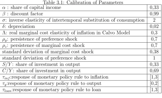
Table 3.1: Calibration of Parameters
α : share of capital income 0,33 β : discount factor 0,99 σ: inverse elasticity of intertemporal substitution of consumption 2
δ: depreciation 0,02
Λ: real marginal cost elasticity of inflation in Calvo Model 0,3 ρg: persistence of preference shock 0,7
ρz: persistence of marginal cost shock 0,7
standard deviation of marginal cost shock 0,38 standard deviation of preference shock 1 S/Y : share of investment in output 0,33 C/Y : share of investment in output 0,69 τinf:response of monetary policy rule to inflation [1,3]
τy:response of monetary policy rule to output [0,2]
τloan:response of monetary policy rule to loan [1,3]
Table 3.2: Indeterminate and Some Determinate Combinations Indeterminate Determinate
(τinf = 0, τy = 1, τloan = 1) (τinf = 1.10, τy = 1, τloan= 1)
(τinf = 0, τy = 1, τloan = 0) (τinf = 1.10, τy = 1, τloan= 0)
(τinf = 0, τy = 0, τloan = 1) (τinf = 1.10, τy = 0, τloan= 1)
(τinf = 1, τy = 1, τloan = 0) (τinf = 1.10, τy = 1, τloan= 0)
(τinf = 1, τy = 0, τloan = 0) (τinf = 1.10, τy = 0, τloan= 0)
(τinf = 1, τy = 1, τloan = 1) (τinf = 1.10, τy = 1, τloan= 1)
Calibration of other parameters
3.7
Simulation Results
Result 1 : Determinacy of the model
The model is only determinant when τinf is equal or greater than 1.10.
Otherwise, it gives indeterminate solutions, which is consistent with the re-lated literature. Then, I can conclude that the model is only determinate with active monetary policy, which requires that nominal interest rate re-sponds to inflation more than one-to-one. Moreover, I list indeterminate and some determinate combinations in the Table2.
The model gives determinate solutions even when τloan=0 either τy = 0.
assume that central bank responds actively to loan growth.
These results are consistent under a fixed tax rate changing between 0 and 0.50. The model is not determinate when tax rate is higher than 0.50.
Result 2: At each combination of parameters out of 8000 combi-nations, which comes from the ranges of parameters in which each takes 20 values, Loss is lower when central bank puts a loan tax as a policy rule.
I make the analysis with two ways : In the first way, the methodol-ogy I use is that I start from the calibration in which tax is zero as running the loop as described before. Then, I replicate the simulations for increasing tax values. Up to the point that tax is equal or greater than 0.50, the model is determinate and the value of loss function is lower at each simulation for different calibrations in which tax rate varies.
1. When tax is zero, the optimum policy rule parameters are as the fol-lowing:
(τinf, τy, τloan)=(1.2,1.9,1.10)
tax=0 and minimum mean Loss=0.0510, (in terms of real numbers Loss=1.0523)
2. With this optimum combination of parameters , I further simulate the model with different tax values. The results of the simulation are as the following:(τinf, τy, τloan) =(1.2,1.9,1.10)
(a) tax =0.10 minimum mean Loss=0.0471 (in terms of real numbers Loss=1. 0482)
(c) tax=0.30 minimum mean Loss=0.0401 (in terms of real numbers Loss=1. 0440)
According to the simulation results, we see that there must be an optimum tax rate (greater than zero) to gain lower loss values. In this case , it must be between 0.30-0.50 since loss is decreasing in tax rate up to the point where tax rate is 0.50.
Result 2 with different methodology: After optimization over policy rule parameters in which tax rate is zero, I take this parameters as given. Next, I define tax rate as an endogenous variable which depends on deviations from steady state from output and inflation, and loan growth, implying that central bank changes the tax rate according to the economic conditions. Then, I write a loop over the new parameters of tax rate equa-tion and simulate for this loop. Consequently, simulaequa-tion results show that inclusion of tax rate leads lower loss values.
˜
γt = m ˜πt+ n ˜Yt+ g(Loant+1− Loant) (3.49)
where m, n, g are the elasticities of tax rate with respect to deviations from steady state from output and inflation, and loan growth respectively. I con-strain each of them as between 0 and 1 and consider the simulation results in which tax is greater than zero.
1. When tax is zero , the optimum policy rule parameters are as the following:(τinf, τy, τloan )=(1.2,1.9,1.10)
tax=0 and minimum mean Loss=0.0510,(in terms of real numbers Loss=1.0523)
Loss=1.0177)
3.8
Graphics of Simulation
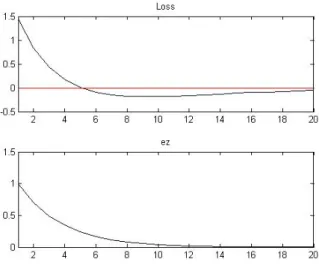
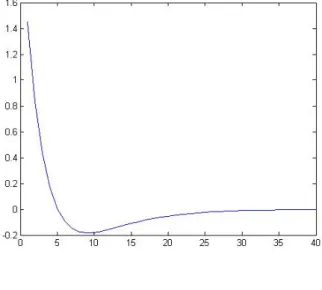
a) In two cases, when tax is zero, impulse responses to a marginal cost shock and losses are given as such:
Figure 3.1: Impulse responses to a marginal cost shock when tax=0
Figure 3.2: Changes in mean of loss values responding to a marginal cost shock when tax=0
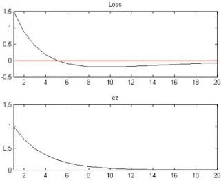
Figure 3.3: Impulse responses to a marginal cost shock when tax=0.20
Figure 3.4: Changes in mean of loss values responding to a marginal cost shock when tax=0.20
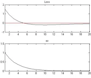
Figure 3.5: Impulse responses to a marginal cost shock when tax=0.30
Figure 3.6: Changes in mean of loss values responding to a marginal cost shock when tax=0.30
d) An endogenous taxation equation, tax is between zero and unity, Loss
Figure 3.7: Loss Tax
CHAPTER 4
CONCLUSION
In the case that monetary policy authority considers excessive loan growth as a potential threat to financial stability, an alternative way to take it into account is to make the loan growth be a component of the loss function. Then, under commitment, it seeks for the interest rate rule via optimizing the weights in the loss function. In this set up, the simulation results sug-gest that an endogenous taxation provides lower mean values of loss function since there exists an optimum tax rate for any optimum combinations of pol-icy rule parameters. On the other hand, trying to achieve both financial stability and price stability by penalizing excessive loan growth only in a Taylor-type interest rate rule causes higher mean values function since there exist trade-off issues among components of the interest rate rule. That is, an increase in interest rates in response to loan growth raises the renting cost of capital, leading to cost-push inflation. Therefore, it creates a conflict of stability purposes. Moreover, giving more weights than optimal values in the interest rate rule increases mean values of loss function. However, incorpo-rating a loan tax that responds to output, inflation and loan growth allows to further penalize excessive loan growth instead of giving more weights on loan growth in the interest rate rule. Accordingly, a loan tax that responds to output,inflation and loan growth is welfare-improving in the presence of
leaning against financial winds policy. In other words, in order to sustain both financial stability and price stability, a loan tax and and an augmented Taylor that respond to output, inflation and loan growth form the optimal monetary policy combination.
BIBLIOGRAPHY
Angelini, P., Neri S. and Fabio Panetta (2012) : ”Monetary and Macro-prudential Policies”, European Central Bank Working Paper Series No: 1449.
Adrian, S. and H. Song (2011): ”Procyclical Leverage and Value-at-Risk”, Federal Reserve Bank of New York Staff Report No: 338.
Beau, D., Clerc L. and B. Mojon (2012): ”Macro-Prudential Policy and the Conduct of Monetary Policy”, Banque de France Working Paper No: 390.
Bernanke, Ben S.and M. Woodford (1997):” Inflation Forecasts and Mone-tary Policy ”, NBER Working Paper No: w6157.
Borio, C. and P. Lowe (2001) : ”Marrying the macro- and Micro-prudential Dimensions of Financial stability”, BIS Papers No:1.
Borgy, V., Clerc L. and Renne, P.(2009) :”Asset-price Boom-Bust Cycles and Credit: What Is the Scope of Macro-prudential Regulation?”, Banque de France Working Papers No:263.
Calvo, Guillermo A. (1983): ”Staggered Prices in a Utility-Maximizing Framework” Journal of Monetary Economics12: 383-398.
Carlstrom, Charles T., Timothy S. Fuerst (2005): ”Investment and Interest Rate Policy: A Discrete Time Analysis”, Journal of Economic Theory 123:4-20.
Clarida, R., Gali J. and M. Gertler (1999): ”The Science of Monetary Pol-icy: A New Keynesian Perspective”,Journal of Economic Literature 37:1661-1707.
Eichengreen, B. and C. Arteta (2002): ”Banking Crises in Emerging Mar-kets: Presumptions and Evidence”, Center for International and Devel-opment Economics Research (CIDER) Working Papers ) No:C00-115. Reinhart, C., Graciela L. Kaminsky (1999): ”The Twin Crises: The Causes
of Banking and Balance-of-Payments Problems”, American Economic Association 89(3):473-500.
Fisher, I. (1933) : ”The Debt-Deflation Theory of Great Depressions”, Econometrica 1(4):337-57.
Galati, G. (2010): Macroprudential Policy, A literature Review, De Neder-landsche Bank Working Paper No:267.
Kannan, P., Rabanal P. and M.Scot (2009): ”Monetary and Macroprudential Policy Rules in a Model with House Price Booms”, IMF Working Papers 12:1-36.
Kerr, William R. and Robert G. King (1996): ”Limits on Interest Rate Rules in the IS-LM Model”, Federal Reserve Bank of Richmond Economic Quarterly Spring.
Kiyotaki, N. and J.Moore (1997): ”Credit Cycles”, The Journal of Political Economy 105(2):211-248.
Lambertini, L., Mendicino C. and M. Teresa Punzi (2013): ”Leaning Against Boom-Bust Cycles in Credit and Housing Prices”, Journal of Economic Dynamics and Control 37(8): 1500-1522.
Mendoza, G. and Terrones, E. (2008): ”An Anatomoy of Credit Booms: Evidence From Macro Aggregates and Micro Data”, NBER Working Paper No:w14049.
Modigliani, F. and Miller, M. (1958): ”The Cost of Capital, Corporation Finance and the Theory of Investment”, American Economic Review 48(3):261297.
Taylor, John B. (1993): ”Discretion versus Policy Rules in Practice”, Carnegie-Rochester Conference Series on Public Policy 39:195214.
Yun, Tack (1996) : ”Nominal Price Rigidity, Money Supply Endogeneity, and Business Cycles”, Journal of Monetary Economics 37(2):345-370.
APPENDIX
In this part, I figure two alternative calibration studies at certain tax levels, and then seek for a more efficient tax rate via the same methodology I have employed before.
A)
1. When tax rate is 0.20, the optimum policy rule parameters are as the following:(τinf, τy, τloan)=(1.3,1.9,1.10)
when tax rate=0.20 and minimum mean Loss=0.0394, (in terms of real numbers Loss=1.0401)
2. With this optimum combination of parameters , I further simulate the model with different tax values. The results of the simulation are as the following:
(a) when tax rate =0.30 minimum mean Loss=0.0365 (in terms of real numbers Loss=1.0371)
(b) when tax rate is in between (0.30,0.50) minimum mean Loss=0.0186 (in terms of real numbers Loss=1.0119)
B)
1. When tax rate is 0.30, the optimum policy rule parameters are as the following:(τinf, τy, τloan)=(1.4,1.9,1.10)
when tax rate=0.30 and minimum mean Loss=0.0330, (in terms of real numbers Loss=1.0335)
2. With this optimum combination of parameters, I further simulate the model with different tax values. The results of the simulation are as the following:
when tax rate is in between (0.30,0.50) minimum mean Loss=0.0180 (in terms of real numbers Loss=1.0181)