Hyung Joong Kim, Saurav Z K Sajib, Woo Chul Jeong et al. MREIT using low amplitude current
Ozlem Birgul, Mark J Hamamura, L Tugan Muftuler et al.
IOP PUBLISHING PHYSICS IN MEDICINE AND BIOLOGY
Phys. Med. Biol. 55 (2010) 3177–3199
doi:10.1088/0031-9155/55/11/013
Fourier transform magnetic resonance current density
imaging (FT-MRCDI) from one component of
magnetic flux density
Yusuf Ziya Ider1, Ozlem Birgul2, Omer Faruk Oran1, Orhan Arikan1, Mark J Hamamura3 and L Tugan Muftuler3
1 Department of Electrical and Electronics Engineering, Bilkent University, Ankara, Turkey 2 TUBITAK UZAY, METU Campus, Ankara, Turkey
3 Center for Functional Onco-Imaging, University of California, Irvine, CA, USA
E-mail: [email protected]
Received 6 December 2009, in final form 8 April 2010 Published 17 May 2010
Online at stacks.iop.org/PMB/55/3177
Abstract
Fourier transform (FT)-based algorithms for magnetic resonance current density imaging (MRCDI) from one component of magnetic flux density have been developed for 2D and 3D problems. For 2D problems, where current is confined to the xy-plane and z-component of the magnetic flux density is measured also on the xy-plane inside the object, an iterative FT-MRCDI algorithm is developed by which both the current distribution inside the object and the z-component of the magnetic flux density on the xy-plane outside the object are reconstructed. The method is applied to simulated as well as actual data from phantoms. The effect of measurement error on the spatial resolution of the current density reconstruction is also investigated. For 3D objects an iterative FT-based algorithm is developed whereby the projected current is reconstructed on any slice using as data the Laplacian of the z-component of magnetic flux density measured for that slice. In an injected current MRCDI scenario, the current is not divergence free on the boundary of the object. The method developed in this study also handles this situation.
1. Introduction
Current density imaging (CDI) is the inverse problem of reconstructing a current density distribution, J(x,y,z), from its magnetic field, H(x,y,z). Measurement of this magnetic field may be achieved by one of the several technologies most of which only allow for the measurement of the magnetic field outside the current-carrying object. In MRCDI, a magnetic resonance imaging (MRI) system is utilized to measure the magnetic field inside the currentcarrying object and better sensitivity from source to measurement is achieved. In general if
0031-9155/10/113177+23$30.00 © 2010 Institute of Physics and Engineering in Medicine Printed in the UK 3177 all three components of the magnetic field, Hx,Hy,Hz, are measured then current density can be reconstructed by J = ∇ × H. However in MRCDI, only Hz can be measured, where the z-axis is defined as the direction of the main static magnetic field of the MRI system. Rotations of the object in the MRI gantry are needed if Hx and Hy are to be measured also. However, rotation of the object in a conventional MRI system may not be possible, nor may it be desirable due to object misalignments and distortions. It is therefore preferable to attempt the reconstruction of current density from Hz measurement only, which is the purpose of this study. (What is actually measured using an MRI system is the magnetic flux density, Bz. However in the following, all mathematical derivations are made in terms of the magnetic field H since B = μH and we assume throughout the paper that μ is space invariant and has the free space value μ0 = 4π × 10−7H m−1.)
Several spatial domain algorithms for MRCDI have been proposed. Some investigators have treated the MRCDI problem as a separate one (Scott et al 1991, 1992, Joy et al 1989, Eyuboglu et al 1998), but others have approached it as a companion problem to MREIT where internal conductivity distribution and internal current density are reconstructed simultaneously (Oh et al 2003a, 2003b, Seo et al 2003a, 2003b, Hasanov et al 2004, Pyo et
al 2005). In the latter group, an additional auxiliary current injection is necessary. Pyo et al (2005) and Park et al (2007) have analyzed to what extent current density can be recovered from Hz only. Park et al (2007) have shown that for 3D problems, recovery of current density from ∇2Hz does not have a unique solution but there is a recoverable component which they call the ‘projected current’. Lee et al (2003) and Oh et al (2003a) have used Fourier transform (FT) methods for MRCDI. Other investigators have used FT methods for the CDI problem in which the magnetic field is measured outside the object using non-MRI methods (Roth et al
1989, Wijngaarden et al 1998, Sezginer 1987). Pesikan et al (1990) have also used Fourier domain methods for the CDI problem and they have used MRI to measure the magnetic field but their measurements are confined to a region away from the current sources.
Roth et al (1989) have studied the problem of imaging a 2D current distribution from its magnetic field measured by a magnetometer on a plane above the plane of the currents. They have derived the Fourier domain forward and inverse transfer functions, from currents to the magnetic flux density and from the magnetic flux density to the currents respectively. They have performed simulations to investigate the limitations of their reconstruction algorithm. Even for a current distribution confined to a finite sized object, the magnetic flux density is negligible only beyond a certain distance away from the object. Therefore, Roth et al have chosen to measure the magnetic flux density in a 6.4 × 6.4 mm area for a current distribution confined to a 1 × 1 mm area. This requirement may be met by a magnetometer-based measurement system which aims at measuring the magnetic flux density outside the object. However in MRCDI, MRI is used to measure the magnetic flux density only inside the object. Although it may also be possible to measure the magnetic flux density outside the object using
3178 Y Z Ider et al
MRI by surrounding the object by water-filled pads, this is an impractical procedure to follow in real applications. Therefore, the method of Roth et al needs to be extended to cases whereby the magnetic field is measured inside the object only. Roth et al (1989) have also assumed that the current distribution is divergence free. This condition is not met in injected current MRCDI in which, although the current is divergence free inside the object, it is not divergence free on the boundary where current is injected via electrodes attached to the boundary of the object.
In Lee et al (2003) and Oh et al (2003a), a special geometry is considered in which current has only one component and this current component is related to only one component of the magnetic flux density in the Fourier domain. Thus, the methods developed by Lee et al (2003) and Oh et al (2003a) are applicable to limited problems of special geometry. In any case, it is
worth noting that in their studies as well, magnetic flux density is supposed to be measured in a larger area than covered by the area in which the current density is confined.
Pesikan et al (1990) have measured the magnetic flux density of a planar current distribution on a plane above the plane of the currents (the xy-plane), using MRI. In their study, current is restricted to the surface of a printed circuit board which is bathed in nonconducting mineral oil to provide an MR signal. They have measured Bz at a height of 1 cm above the circuit board. They have analyzed the factors which determine the spatial resolution of current density reconstruction and have shown how resolution is affected by the signal-to-noise ratio (SNR) of the measurements and the height at which the measurements are made. Our study differs from that of Pesikan et al in that we measure the magnetic field on the plane of the currents.
In this study, a FT-based method for MRCDI is developed. The algorithm is first formulated for the 2D case where current has only transversal (x- and y-) components which do not have z-dependence. For solution of such problems, an iterative method (iterative FTMRCDI) is proposed. This method makes use of the magnetic flux density measurements inside the object only, and it can also be used to reconstruct the magnetic flux density outside the object. Furthermore, the method handles the fact that current is not divergence free on the boundary of the object. The iterative FT-MRCDI method for 2D problems is applied to reconstruction of current density from simulated magnetic flux density data as well as from real data obtained from phantoms. The FT-MRCDI method is then extended to the general 3D case and assumptions under which this problem can be solved are explored. An iterative algorithm is proposed whereby ‘projected current’ is reconstructed from simulated ∇2Bz data.
2. Methods
2.1. Iterative FT-MRCDI for 2D problems
2.1.1. Problem definition. Let be a connected and bounded domain in R2 (defined by the xy-plane, or the z = 0 plane) with boundary . Let S represent a slab of thickness d defined by the
set with the current injection boundary surface
. Assuming that the current injection density on T and the conductivity in S do not have z-dependence, current density, electric field and potential field in S also do not have z-dependence. With unit outward normal along the boundary being n, and non-zero conductivity in S being σ(x,y) in units of S m−1, the potential field, (x,y), obeys Laplace’s equation
0 in (1)
and satisfies the Neumann condition
on , (2)
where , and g is the boundary injected current density in A m−2 and its integral on is zero.
The current density J (A m−2) and electrical field E are given by J = σE and E . We define J(x,y) for all (x,y) ∈ R2 but it is zero if (x,y) does not belong to . The magnetic field
due to J has only the z-component on the xy-plane and is given for the whole xy-plane by the
Biot–Savart integral
. (3) This equation is a Fredholm integral equation of the first kind and is ill-posed in general. The inverse problem of MRCDI is to find Jx and Jy from available measurements of Hz(x,y,0) on a finite number of spatial locations in .
2.1.2. Iterative FT-based MRCDI inversion technique. The 2D FT (F2) of Hz(x,y,0) is defined as
(4) where kx and ky are the spatial frequencies (1/m) along x and y respectively. Using the forward filter functions derived in the appendix, F2{Hz(x,y,0)} can be written in terms of the FT of the
x and y components of the current density as
F2{Hz(x,y,0)} = F(kx,ky)(−jkyF2{Jx} + jkxF2{Jy}), where
(5)
. (6)
As shown in the appendix, if d is very small and if d is very large .
Divergence of the current density is zero in and as explained in the appendix, it can be taken to be where (x,y) is the impulse function defined on (Onural 2006). Since current density is zero outside in R2. Taking the 2D FT of both sides, we obtain
j2 , (7) where
is the incremental distance on . From equations (5) and (7), one can derive
(8) and
. (9)
Let us now define the difference currents, Jxd = Jx − Jxu and Jyd = Jy − Jyu, where Jxu and Jyu are the current density distributions for a uniform conductivity distribution, σu. Note that the actual value of σu does not alter Jxu and Jyu. Since the divergences of the actual current and the current for σu are the same, we have a divergence-free difference current. Thus,
and
(10) ,
where is the difference between the measured magnetic field at z = 0 and the magnetic field calculated from and 0. Therefore, the inverse filters Fx(kx,ky) and
Fy(kx,ky) to be used to find from , respectively, are
defined as and . (11) If d is small, we have 1 j2ky 1 j2kx =and Fy(kx,ky) = −(12) Fx(kx,ky) d d
and if d is large, we have Fx(kx,ky) = j2πky
In a truly 2D problem where become undefined and we must study what happens when d → 0. For a given amount of applied current, as d → 0, the current density inside the object approaches ∞. However, dJ approaches Js which is now surface current density in units of A
m−1. Multiplying the expressions by d we have d
and d
and dJyd → J
ysd yielding the
expressions ,
where Jxsd and Jysd are the x- and y-components of the difference surface current density. In conclusion the inverse filter functions which relate the surface difference current density to
the measured magnetic flux density become , and .
Note that the inverse filter functions Fx(kx,ky) and Fy(kx,ky) (and for that matter Fx0(kx,ky) and Fy0(kx,ky))) are undefined at kx = ky = 0. As shown in the appendix, the dc values of and
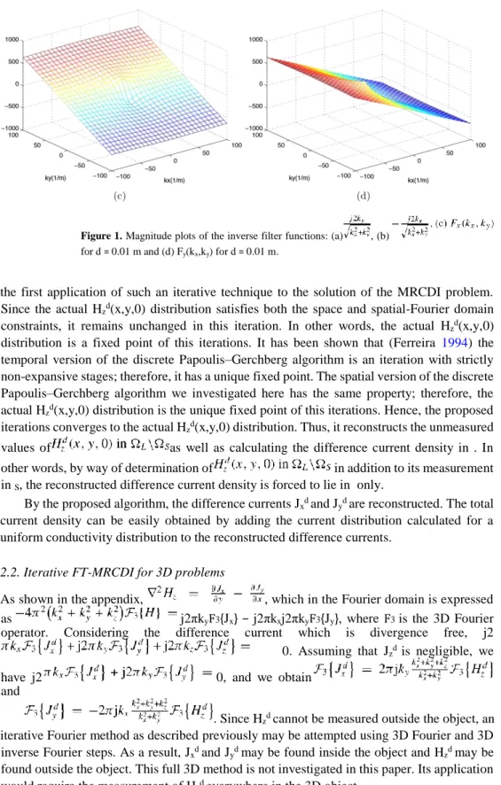
are zero. Therefore, we can take Fx(0,0) = Fy(0,0) = 0 (and Fx0(0,0) = Fy0(0,0) = 0). The filters for d = 0 and for d = 0.01 m are shown in figure 1.
Althoughcurrentsareconfinedto existsinthewholexy-plane. UsingMRI, in practice, Hzd(x,y,0) is measured only in . In this study, we have developed an iterative method whereby the Jxd and Jyd are reconstructed in measurements made in only. This iterative method also reconstructs Hzd(x,y,0) outside .
Let us assume that Hzd(x,y,0) is negligible beyond a sufficiently large region L such that . Due to practical reasons which will be explained in section 3, measurements of Hzd(x,y,0) on an even smaller region S such that may be used. The assumed conditions and the major steps of the algorithm are given as follows:
(i) Hzd(x,y,0) is assumed to be zero in is calculated.
(iii) Using the filters Fx and Fy, are calculated. Then, by inverse FT Jxd and Jyd are calculated in L.
(iv) The calculated currents are then confined to by multiplying by a masking function which is 1 in but is 0 in . is calculated back from the current density confined to using equation (5) and inverse FT.
(vi) Unless a convergence criterion for is met, the obtained values for
in are retained, but the values obtained for are replaced by the measured values, and steps (ii) through (vi) are repeated.
The proposed algorithm performs iterations in space and spatial-Fourier domains similar to the famous Papoulis–Gerchberg algorithm which performs iterations in time and temporalFourier domains (Gerchberg 1974 and Papoulis 1975), which has found many application areas (Sanz and Huang 1983). To the best of our knowledge, the proposed algorithm is
Figure 1. Magnitude plots of the inverse filter functions: (a) , (b) for d = 0.01 m and (d) Fy(kx,ky) for d = 0.01 m.
the first application of such an iterative technique to the solution of the MRCDI problem. Since the actual Hzd(x,y,0) distribution satisfies both the space and spatial-Fourier domain constraints, it remains unchanged in this iteration. In other words, the actual Hzd(x,y,0) distribution is a fixed point of this iterations. It has been shown that (Ferreira 1994) the temporal version of the discrete Papoulis–Gerchberg algorithm is an iteration with strictly non-expansive stages; therefore, it has a unique fixed point. The spatial version of the discrete Papoulis–Gerchberg algorithm we investigated here has the same property; therefore, the actual Hzd(x,y,0) distribution is the unique fixed point of this iterations. Hence, the proposed iterations converges to the actual Hzd(x,y,0) distribution. Thus, it reconstructs the unmeasured values of as well as calculating the difference current density in . In other words, by way of determination of in addition to its measurement in S, the reconstructed difference current density is forced to lie in only.
By the proposed algorithm, the difference currents Jxd and Jyd are reconstructed. The total current density can be easily obtained by adding the current distribution calculated for a uniform conductivity distribution to the reconstructed difference currents.
2.2. Iterative FT-MRCDI for 3D problems
As shown in the appendix, , which in the Fourier domain is expressed as j2πkyF3{Jx} − j2πkxj2πkyF3{Jy}, where F3 is the 3D Fourier operator. Considering the difference current which is divergence free, j2
0. Assuming that Jzd is negligible, we
have j2 0, and we obtain
and
. Since Hzd cannot be measured outside the object, an iterative Fourier method as described previously may be attempted using 3D Fourier and 3D inverse Fourier steps. As a result, Jxd and Jyd may be found inside the object and Hzd may be found outside the object. This full 3D method is not investigated in this paper. Its application would require the measurement of Hzd everywhere in the 3D object.
If we have measured Hzd in only one transversal plane, then we can still make some assumptions to apply the theory derived for a 2D problem. Let us assume that Hzd is measured in the z = 0 plane, current is z-independent in a slab defined by , and that current outside this slab does not affect the measured Hzd. In such a case, the theory derived previously can be directly applied to find the current in the slab. However such assumptions may be realistic only for certain object shapes, for certain current application electrode shape, size and positions, and for certain internal conductivity distributions.
Instead of using Hzd measurement as input to the current reconstruction algorithm, one can approach the 3D inverse problem by calculating ∇2Hz first and using it as the input. It should be noted at the onset that ∇2Hz from the current due to uniform conductivity inside the object is zero. Therefore , and from ∇2Hz one cannot find the component of current due to uniform conductivity but can at best find the difference current J
can be expressed in the Fourier domain as
j2 d . Multiplying by e2πjkzt (in order to derive the equations for the z = t plane) and integrating with respect to kz from −∞ to ∞, we obtain
. (14)
d 0. Assuming that is Since the divergence of J
negligible on z = t , we have 0 which can be expressed for the z = t plane as 0. Taking the 2D FT of this last expression, we obtain
j2 . (15)
From equations (14) and (15), we obtain
and
(16) Thus, starting from the measurement of ∇2Hz at z = t, one can find estimates for Jxd(x,y,t) and Jyd(x,y,t) currents at that slice. These are estimates because we have made
d the assumption that (x,y,t) is negligible. Of course, measurement of ∇2Hz at z = t requires at least the measurement of Hz at z = t, z = t + δ and z = t − δ with δ chosen to be sufficiently small so that can be calculated at z = t.
Using the same notation as before, let denotes the interior of the slice of interest, its boundary and L a region such that 0 outside but it may not be zero on . This is evident when it is considered that . Since Jx and Jy are zero just outside , their derivatives will have jumps on when evaluated by a discrete approximation. However, it is not possible to measure because this requires the measurement of Hz slightly outside of . Therefore as a starting point, ∇2Hz is calculated in from the measured Hz. On is taken to be equal to its immediate value in .
Equation (16) is then used to find the currents in L. For the second iteration, the currents are nulled for outside of is calculated from and on . The values of ∇2Hz calculated on are retained but the measured values are assigned to ∇2Hz in . Obviously with this procedure ∇2Hz becomes 0 outside of . As a final step for the second iteration, the currents are calculated again from equation (16). Iterations are continued until the calculated ∇2Hz becomes close to the measured .
The estimates given above for Jxd(x,y,t) and Jyd(x,y,t) will be hereafter called the projected difference current density and will be denoted by Jx∗(x,y,t) and Jy∗(x,y,t), respectively. This terminology is in line with the terminology of Park et al (2007) as explained in section 4.
2.3. Experimental and numerical methods
2.3.1. Hz measurements. The magnetic field measurements were carried out using the 4T whole body MRI system at UCI Center for Functional Onco Imaging. A 16 leg, quadrature, high-pass birdcage coil with 10 cm diameter and 18 cm length was designed and built in-house for the experiments. A current source that uses the pulses generated by the MRI console and a voltage-to-current converter is used to generate a current distribution inside the object. This current source was triggered by a TTL pulse generated by the scanner computer. A pulse sequence, similar to the one proposed by Mikac et al (2001), is used. This sequence is similar to a fast spin echo sequence, where a train of 180◦ RF pulses is applied following a 90◦ RF pulse. No phase encode or read-out gradients were applied between the 180◦ RF pulses and the data were collected with a single read-out gradient only after the last 180◦ RF pulse. The details of the data acquisition system and the pulse sequence are explained in Birgul et al (2006).
2.3.2. Phantompreparation. Inordertotesttheperformanceofthealgorithmexperimentally,
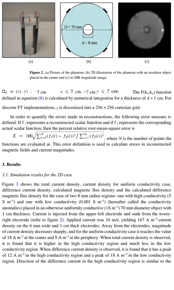
agar-gel phantoms with various conductivity distributions were prepared. A cylinder with 7 cm diameter was filled with 1 cm deep agar-gel. A small hollow cylinder with 8 mm diameter was placed at different locations to understand the spatial dependence of the algorithm. Four copper electrodes with 6 mm width were placed on the inner wall of the outer cylinder every 90◦ degrees. The height of the electrodes was the same as the depth of the phantom so that there is no variation in the z-direction and the phantom approximates a 2D situation. Currentcarrying wires were fixed on the support of the cylinder parallel to the main magnetic field to minimize the z-component of the magnetic field generated inside the object by these wires. The picture and the schematic definition of the phantom are given in figure 2.
2.3.3. Generation of simulated data and filter functions. For 2D problems, finite element
method (FEM) is used to solve the forward problem defined by equations (1) and (2) for 3.5 cm) and thickness d = 1 cm. Comsol Multiphysics package is used for FEM solutions and triangular mesh elements and quadratic shape functions are used. Triangle sizes are less than 1 mm and are as small as 0.4 mm in regions of high conductivity gradient. Once the current density distribution is calculated, Hz is obtained by discretizing the Biot–Savart integral defined in equation (3). For this purpose, the 1 cm thick slab is divided into ten 1 mm subslabs. Hz is calculated in
Figure 2. (a) Picture of the phantom, (b) 2D illustration of the phantom with an insulator object placed in the center and (c) its MR magnitude image.
7 cm 7 cm . The F(kx,ky) function
defined in equation (6) is calculated by numerical integration for a thickness of d = 1 cm. For discrete FT implementations, L is discretized into a 256 × 256 cartesian grid.
In order to quantify the errors made in reconstructions, the following error measure is defined: If f 1 represents a reconstructed scalar function and if f 2 represents the corresponding actual scalar function, then the percent relative root-mean-square error is
, where N is the number of points the functions are evaluated at. This error definition is used to calculate errors in reconstructed magnetic fields and current magnitudes.
3. Results
3.1. Simulation results for the 2D case
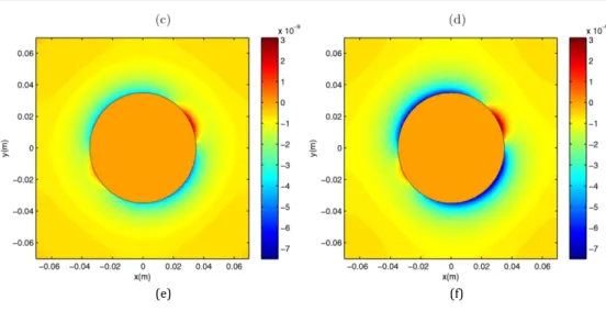
Figure 3 shows the total current density, current density for uniform conductivity case, difference current density, calculated magnetic flux density and the calculated difference magnetic flux density for the case of two 8 mm radius regions: one with high conductivity (5 S m−1) and one with low conductivity (0.001 S m−1) (hereafter called the conductivity anomalies) placed in an otherwise uniformly conductive (1S m−1) 70 mm diameter object with 1 cm thickness. Current is injected from the upper-left electrode and sunk from the lower-right electrode (refer to figure 2). Applied current was 10 mA, yielding 167 A m−2 current density on the 6 mm wide and 1 cm thick electrodes. Away from the electrodes, magnitude of current density decreases sharply, and for the uniform conductivity case it reaches the value of 18 A m−2 at the center and 9 A m−2 at the periphery. When total current density is observed, it is found that it is higher in the high conductivity region and much less in the low conductivity region. When difference current density is observed, it is found that it has a peak of 12 A m−2 in the high conductivity region and a peak of 18 A m−2 in the low conductivity region. Direction of the difference current in the high conductivity region is similar to the
direction of current for the uniform conductivity case but the direction of difference current in the low conductivity region is reversed.
It is observed that the total magnetic flux density extends beyond the 70 mm diameter circular conductive object as expected. The difference magnetic flux density however is mostly confined to the object’s interior although it is not negligible outside as will be shown
Figure 3. (a) Conductivity distribution, (b) total current density, (c) current density for uniform conductivity, (d) difference current density, (e) total magnetic flux density and (f) difference magnetic flux density for a 1 cm thick object which has a low conductivity region of 0.001 S m−1, a high conductivity region of 5 S m−1 and background conductivity of 1 S m−1. The unit for the magnetic flux density is Tesla.
in the next figure. Total magnetic flux density is most pronounced near the current electrodes whereas the difference magnetic flux density is most pronounced around the boundaries of the conductivity anomalies.
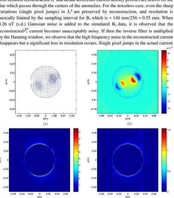
Figure 4 shows the results of reconstruction for the simulation object in figure 3. Five iterations are performed beyond which significant improvement in reconstructed current and magnetic flux density is not observed. Errors in the reconstructed magnetic flux density are 5.5%, 2.7%, 1.7%, 1.2% and 1.0% for the first five iterations. Errors in the reconstructed current density magnitude are 17.7%, 13.3%, 12.2%, 11.8% and 11.8% for the first five iterations. The benefit obtained by applying the iterative algorithm is better observed when the reconstructed distributions are viewed for outside the 70 mm object. Figures 4(e) and (f) show the reconstructed magnetic flux densities outside the object for the first and the fifth iterations respectively; the magnetic flux density is nulled inside in order to emphasize its outside behavior. From the first to the fifth iteration, the reconstructed magnetic flux density outside the object builds up significantly. For the reconstructed current density, it is observed that at the first iteration outside current is still very high (up to 9 A m−2) but in the fifth iteration it is significantly reduced, as shown in figures 4(c) and (d) where inside current is nulled in order to emphasize its outside behavior.
WehaveassumedsofarthatBz measurement does nothave noise, except forthenumerical errors in simulated Bz calculations, evaluation of the filter functions and errors due to the finite sampling rate. We have next investigated the reconstruction success when noise is added to Bz. Noise in Bz measurements using MRI is first investigated by Scott et al (1992). From their formulation, standard deviation of noise in Bz is 2.6 nT, 1.3 nT or 0.65 nT for an MR system which has an SNR of 15, 30 or 60 in magnitude images respectively, and for current injection duration of 48 ms. Although the probability density function of the noise is not Gaussian, most investigators use Gaussian distribution as an approximation (Oh et al (2003b)).
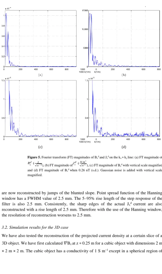
Figure 5 shows the FT magnitudes for Bzd and Jxd on a certain line in the frequency domain (kx = ky line). High frequency components of Bzd are relatively more attenuated compared to the high frequency components of Jxd (similarly for Jyd ). Thus, the Biot–Savart integral acts as a low pass filter and suppresses the high frequency components of the currents. However, the inverse filters shown in figures 1(c) and (d) have high pass behavior to compensate for this suppression. Therefore, the inverse problem is ill conditioned in the sense that if there is high frequency noise in Bz measurement, then error in the reconstructed currents will be amplified. In actual application, the inverse filter must be band limited by multiplying with a low pass filter in order to avoid excessive noise in reconstructed currents. In the same figure, we show the FT of Bzd with 0.26 nT (s.d.) additive Gaussian noise. In this case by visual inspection, it is evident that a low pass filter with 200 m−1 cutoff (−3 dB) must be used because above 200 m−1 the level of signal becomes comparable to or less than the level of wide band noise. We have used a Hanning window, w(kx,ky) = . k max , as used by Roth
et al (1989).
We have taken kmax = 400 m−1 because with this kmax value, the filter has −3 dB cutoff at 200 m−1.
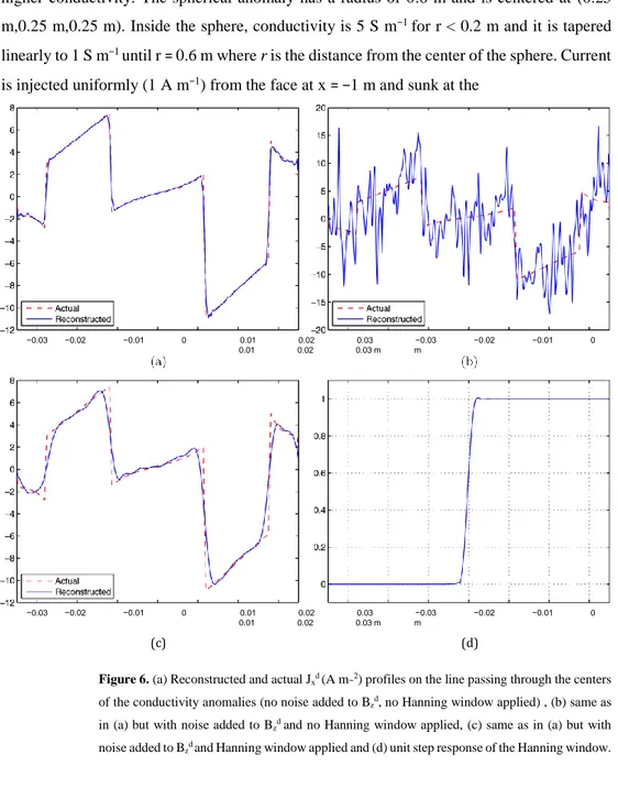
Figure 6 compares the current reconstructions made for noiseless and noisy cases. The fifth iteration reconstructed Jxd and actual difference current density profiles are drawn for the line which passes through the centers of the anomalies. For the noiseless case, even the sharp variations (single pixel jumps) in Jxd are preserved by reconstruction, and resolution is basically limited by the sampling interval for Bz which is = 140 mm/256 = 0.55 mm. When 0.26 nT (s.d.) Gaussian noise is added to the simulated Bz data, it is observed that the reconstructed current becomes unacceptably noisy. If then the inverse filter is multiplied by the Hanning window, we observe that the high frequency noise in the reconstructed current disappears but a significant loss in resolution occurs. Single pixel jumps in the actual current
(e) (f)
Figure 4. Reconstructions for the object shown in figure 3. (a) Difference current density (fifth iteration), (b) difference magnetic field (fifth iteration), (c) magnitude of current density outside the object (first iteration), (d) magnitude of current density outside the object (fifth iteration), (e) difference magnetic field outside the object (first iteration) and (f) difference magnetic field outside the object (fifth iteration). The unit for the magnetic flux density is Tesla, and the unit for current density is A m−2.
0 200 400 600 800 1000 0 200 400 600 800 1000 k(1/m) k(1/m)
0 200 400 600 800 1000 0 200 400 600 800
1000 k(1/m) k(1/m)
(c) (d)
Figure 5. Fourier transform (FT) magnitudes of Bzd and Jxd on the kx = ky line: (a) FT magnitude of ), (b) FT magnitude of ), (c) FT magnitude of Bzd with vertical scale magnified and (d) FT magnitude of Bzd when 0.26 nT (s.d.). Gaussian noise is added with vertical scale magnified.
are now reconstructed by jumps of the blunted slope. Point spread function of the Hanning window has a FWHM value of 2.5 mm. The 5–95% rise length of the step response of the filter is also 2.5 mm. Consistently, the sharp edges of the actual Jxd current are also reconstructed with a rise length of 2.5 mm. Therefore with the use of the Hanning window, the resolution of reconstruction worsens to 2.5 mm.
3.2. Simulation results for the 3D case
We have also tested the reconstruction of the projected current density at a certain slice of a 3D object. We have first calculated ∇2Bz at z = 0.25 m for a cubic object with dimensions 2 m × 2 m × 2 m. The cubic object has a conductivity of 1 S m−1 except in a spherical region of
higher conductivity. The spherical anomaly has a radius of 0.6 m and is centered at (0.25 m,0.25 m,0.25 m). Inside the sphere, conductivity is 5 S m−1 for r < 0.2 m and it is tapered linearly to 1 S m−1 until r = 0.6 m where r is the distance from the center of the sphere. Current is injected uniformly (1 A m−1) from the face at x = −1 m and sunk at the
−0.03 −0.02 −0.01 0 0.01 0.02 0.03 −0.03 −0.02 −0.01 0 0.01 0.02 0.03 m m
−0.03 −0.02 −0.01 0 0.01 0.02 0.03 −0.03 −0.02 −0.01 0 0.01 0.02 0.03 m m
(c) (d)
Figure 6. (a) Reconstructed and actual Jxd (A m−2) profiles on the line passing through the centers of the conductivity anomalies (no noise added to Bzd, no Hanning window applied) , (b) same as in (a) but with noise added to Bzd and no Hanning window applied, (c) same as in (a) but with noise added to Bzd and Hanning window applied and (d) unit step response of the Hanning window.
x = 1 m face. To generate simulation data, the 3D forward problem for the currents is solved using FEM (1120000 tetrahedrons, 196210 nodes and 3062000 degrees of freedom), and Bz is calculated using the Biot–Savart integral. Bz is then sampled on a cartesian grid with a step size of 5 mm and ∇2Hz is calculated using centered differences except on where
forward or backward differences are used. This results in a ∇2Hz which does not have jumps on . This ∇2Hz is used as input to the first iteration of the reconstruction algorithm.
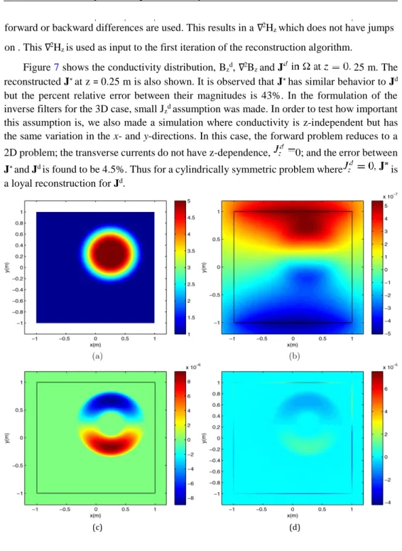
Figure 7 shows the conductivity distribution, Bzd, ∇2Bz and J 25 m. The reconstructed J∗ at z = 0.25 m is also shown. It is observed that J∗ has similar behavior to Jd but the percent relative error between their magnitudes is 43%. In the formulation of the inverse filters for the 3D case, small Jzd assumption was made. In order to test how important this assumption is, we also made a simulation where conductivity is z-independent but has the same variation in the x- and y-directions. In this case, the forward problem reduces to a 2D problem; the transverse currents do not have z-dependence, 0; and the error between J∗ and Jd is found to be 4.5%. Thus for a cylindrically symmetric problem where is a loyal reconstruction for Jd.
−1 −0.5 0 0.5 1 −1 −0.5 0 0.5 1 x(m) x(m)
(e) (f)
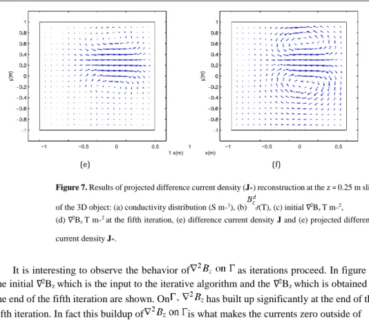
Figure 7. Results of projected difference current density (J∗) reconstruction at the z = 0.25 m slice of the 3D object: (a) conductivity distribution (S m−1), (b) (T), (c) initial ∇2Bz T m−2,
(d) ∇2Bz T m−2 at the fifth iteration, (e) difference current density J and (e) projected difference current density J∗.
It is interesting to observe the behavior of as iterations proceed. In figure 7, the initial ∇2Bz which is the input to the iterative algorithm and the ∇2Bz which is obtained at the end of the fifth iteration are shown. On has built up significantly at the end of the fifth iteration. In fact this buildup of is what makes the currents zero outside of
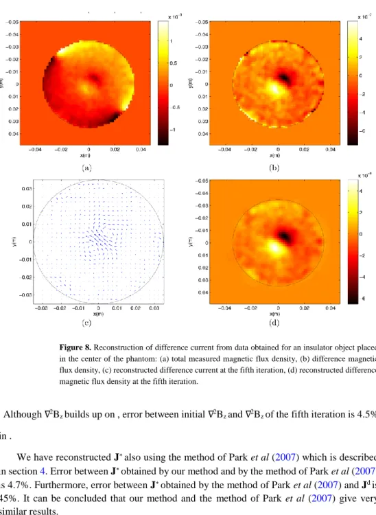
Figure 8. Reconstruction of difference current from data obtained for an insulator object placed in the center of the phantom: (a) total measured magnetic flux density, (b) difference magnetic flux density, (c) reconstructed difference current at the fifth iteration, (d) reconstructed difference magnetic flux density at the fifth iteration.
. Although ∇2Bz builds up on , error between initial ∇2Bz and ∇2Bz of the fifth iteration is 4.5% in .
We have reconstructed J∗ also using the method of Park et al (2007) which is described in section 4. Error between J∗ obtained by our method and by the method of Park et al (2007) is 4.7%. Furthermore, error between J∗ obtained by the method of Park et al (2007) and Jd is 45%. It can be concluded that our method and the method of Park et al (2007) give very similar results.
3.3. Experimental results
The iterative FT-MRCDI method is then applied to data collected from the 2D phantom described in figure 2. Total current of 1 mA is injected from the upper-left electrode and sunk from the lower-right electrode. Figure 8 shows the measured total magnetic flux density, and the difference magnetic flux density obtained by subtracting the calculated uniform magnetic
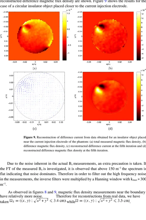
flux density, for the case of a circular insulator object placed at the center of the phantom. Also in the same figure, fifth iteration reconstructed difference current density and reconstructed difference magnetic flux density are shown. Figure 9 shows the results for the case of a circular insulator object placed closer to the current injection electrode.
(c) (d)
Figure 9. Reconstruction of difference current from data obtained for an insulator object placed near the current injection electrode of the phantom: (a) total measured magnetic flux density, (b) difference magnetic flux density, (c) reconstructed difference current at the fifth iteration and (d) reconstructed difference magnetic flux density at the fifth iteration.
Due to the noise inherent in the actual Bz measurements, an extra precaution is taken. If the FT of the measured Bz is investigated, it is observed that above 150 m−1 the spectrum is flat indicating that noise dominates. Therefore in order to filter out the high frequency noise in the measurements, the inverse filters were multiplied by a Hanning window with kmax = 300 m−1.
As observed in figures 8 and 9, magnetic flux density measurements near the boundary have relatively more noise. Therefore for reconstructions from real data, we have
4. Discussion and conclusion
An iterative FT-based algorithm for 2D MRCDI is proposed and successful reconstructions obtained from both simulated data and real phantom data have been presented. Extension of the technique to the 3D case is not trivial. However, an iterative FT-based algorithm is developed to find the projected current density at a certain slice using ∇2Hz data measured for that slice. When applied to actual problems such as human imaging, both the MRCDI and the MREIT problems are inherently 3D in nature (Ider and Onart 2004). It is known that in the general 3D situation, the MRCDI problem does not have a unique solution (Pyo et al 2005, Park et al 2007). However, Nam et al (2008) have shown that a projected current solution for the 3D MRCDI problem may still be useful or even sufficient to find the solution of the 3D MREIT problem.
FT methods for MRCDI have been used by other investigators as well. In Lee et al (2003) and Oh et al (2003a), a special geometry is considered in which one component of the magnetic flux density is related to one component of current only. In Lee et al (2003), current has z-component only, and in Oh et al (2003a) current is predominantly in the z-direction. It is known that F3{Jz} = 2πjkxF3{Hy} − 2πjkyF3{Hx}. Assuming that Hz is negligible, and since magnetic flux density is divergence free, and assuming that μ is uniform, one obtains 2πjkxF3{Hx} + 2πjkyF3{Hy} = 0 . Therefore, one can relate F3{Jz} to F3{Hx} only. Thus, the methods developed by Lee et al (2003) and Oh et al (2003a) are not applicable to the problem considered in this study.
Similar geometry as used in this study for 2D problems has been used by investigators in other areas (Wijngaarden et al 1998, Sezginer 1987). The difference in our study is that magnetic flux density is assumed to be measured inside, whereas in geophysics (Sezginer
1987) or in superconductivity research (Wijngaarden et al 1998), magnetic flux density is measured outside the object.
Roth et al (1989) and Pesikan et al (1990) have studied the reconstruction of planar currents from magnetic flux density measurements made on a plane above the plane of the currents. They have shown that as the distance between measurement plane and the plane of currents is decreased, the resolution of reconstruction increases. In this study, the magnetic flux density is measured on the plane of the currents. We have shown that if there is no measurement noise, resolution is limited by numerical and sampling errors. We have also calculated the magnetic flux density 0.5 cm above the current slab of thickness d = 1 cm. This magnetic flux density is attenuated and smoothed compared to the magnetic flux density measured at the middle plane of the slab. When 2.6 nT (s.d.) noise is added, it is observed that thehighfrequencycomponentsofthemagneticfluxdensitystaybelowthenoisespectrumafter 80 m−1. If a Hanning window with −3 dB cutoff at 80 m−1 is then used, the reconstruction resolution will be around 6.25 mm as compared to 2.5 mm for when magnetic flux density is measured in the center plane of the slab and a Hanning window with −3 dB cutoff at 200 m−1 is used.
Two-dimensional applications such as those described by Wijngaarden et al (1998) and Pesikan et al (1990) have the limitation that the magnetic field cannot be measured on the planeofcurrentsusingconventionalMRIbecausethecurrent-carryingmediumissolidinthose applications. We have not come across any application where the problem is 2D in nature and the current-carrying medium is liquid-like to provide the MR signal. 2D applications for
materials testing or biological specimen investigation where preparation of a slice object is possible may emerge in the future. However, the 2D algorithms developed in this study are also applicable to 3D problems under certain assumptions as explained in section 2.2. Furthermore in future work, the iterative 2D algorithm developed in this study may be extended to cases where the magnetic field is measured above the plane of the currents.
We have reconstructed the difference current density in the 2D case. An alternative approach is to find the FT of gδ and use it in equations (8) and (9) to find the FT of the total current density F2{Jx} and F2{Jy}. Finding the Ft of gδ is however prone to numerical errors even if a high spatial frequency sampling is used because gδ is defined on a thin line coincident with the boundary.
Park et al (2007) have analyzed the recovery of current density in a 3D object. They have developed a theory whereby the ‘projected current’ density is calculated from ∇2Hz measurements instead of Hz measurements. They formulate that total current density, JT , is
the sum of three components, namely JT = J0 +J∗ +JN, where J0 is the current calculated for the object assuming uniform conductivity inside and using the Neumann boundary conditions imposed by the injected current, J0 + J∗ is the projected current, and JN is the component of current which cannot be recovered from ∇2Hz measurement only because it is in the null space of the forward transformation from J to ∇2Hz satisfying the boundary conditions due to theinjectedcurrent. Themagnitudeofthisunrecoverablecomponentisrelatedtothedifference of the Jz current and the z-component current for the uniform conductivity case, Jz0. With the assumption that JN is small, the projected current is a good estimate of the actual total current. The divergence-free transversal current, J∗ is calculated as J where βt(x,y) obeys the differential equation
with the null Dirichlet condition on the boundary defined by the intersection of the object boundary with the z = t plane.
The theory of Park et al (2007) and the FT-MRCDI technique presented in this paper are closely related. Defining β(x,y,z) = βz(x,y), in the Fourier domain we
have , and therefore .
Assuming that Hz at a certain plane, say z = 0, is affected by only the current density in the slab defined by and that and thus β do not have zdependence in
that slab, . Integrating with respect to kz from −∞ to ∞,
we get , and therefore
. Finally and
. These expressions are the same as what we have stated in equation (10).
Park et al (2007) have developed their theory for reconstructions from ∇2Hz data directly. Let f(x, y) denote the ∇2Hz data measured at z = 0. Then from Park et al (2007) theory
and in the Fourier domain .
Therefore, . These
−
expressions are identical to what we have stated in equation (16).
The method developed in this study is more suitable for the problem of induced current MR-CDI (Ozparlak and Ider 2005). In induced current, MR-CDI current is not injected but is induced by an applied magnetic field. Thus, the current density in the object is divergence free both inside and on the boundary.
This work is supported by TUBITAK 107E260 and NIH/NCI R01 CA114210 grants.
Appendix. Derivation of forward filters for the 2D problem ∇ × H = J ∇ × ∇ × H = ∇ × J (A.1) 2 ∇(∇ · H) − ∇ H = ∇ × J 2 ∇ H = −∇ × J and . (A.2)
The 3D-FT pair is defined as
(A.3) Since current is confined to a slab of thickness d,
(A.4) and similarly for F3{Jy}. In the Fourier domain, equation (A.2) becomes
(A.5) and therefore
(A.6) Since
we have
(A.8) If d is large, dsinc(kzd) approaches δ(kz) and
(A.9) If d is small, dsinc(kzd) approaches d and
(A.10) Derivation of equation (7)
In order to illustrate the philosophy behind the derivation of equation (7), let us consider the simple 2D connected and bounded domain (defined by the xy-plane) with boundary . Let us define the problem = , with the Neumann boundary condition , such that f(x,y) = ξ for
for
0 otherwise,
(A.11)
where ξ is the current source density with units of A m−2 and ε is a small positive real number. As 0, with the condition that where G has units of A m−1, f(x,y) → G[δ(x + L) − δ(x − L)]rect where δ(x) is the one-dimensional impulse function and rect(y) is 1 for
and 0 elsewhere. Defining g(x,y) = 0 for y = ±L
= G for x = −L,
= −G for x = L, (A.12)
we can express the partial differential equation as (x,y), where δ is an impulse function on the curve such that it is 0 outside and for any well-behaving
function h which is the line integral of h(x, y)
on where dγ is the incremental distance on . Impulse functions over curves and surfaces are defined and explained by Onural L (2006).
= − L)]rect 2L = −
and it is zero in the interior of .
This impulsive divergence on can be converted to an equivalent boundary condition. Using the divergence theorem, one can show that −Jx(−L−,y) + Jx(−L+,y) = −G. Since σ = 0 outside , we have Jx(−L+,y) = −G. This result can also be expressed as n · J = G on x = −L. Similarly, we have Jx(L−,y) = −G and n · J = −G on x = L. In general
n .
In conclusion the problem can now be viewed as J = g(x,y) on
. This is equivalent to .
Thus, in general, the
original problem
definition expressed by equations (1) and (2) is equivalent to which is equal to
. DC values of Jxd and Jyd
Consider a vertical (x = constant) line in the xy-plane such that its intersection with the conductive connected and bounded domain L is not empty. Consider now another
connected domain with boundary ϒ, in the xy-plane, such that . In other words, most of ϒ lies outside , and the part of ϒ that lies in is the vertical line segment L.
Since current is zero outside , the line integral of the normal component of Jd on ϒ is equal to (depending on the direction of the normal vector on L). From the divergence theorem, the line integral of the normal component of Jd on ϒ is equal to the surface integral of the divergence of J . We know that the divergence of Jd is zero everywhere, and therefore
The dc value of is defined as . Since ,
evaluation of the dc value of comprises line integrals of along all vertical line segments in . We can therefore conclude that the dc value of is zero. Similarly for .
References
Birgul O, Hamamura M J, Muftuler L T and Nalcioglu O 2006 Contrast and spatial resolution in MREIT using low amplitude currents Phys. Med. Biol. 51 5035–49
Eyuboglu M, Reddy R and Leigh J S 1998 Imaging electrical current density using nuclear magnetic resonance Elektrik 6 201–14
Ferreira P J S G 1994 Interpolation and discrete Papoulis–Gerchberg algorithm IEEE Trans. Signal Process. 42 2596–
606
Hasanov K F, Ma A W, Yoon R S, Nachman A I and Joy M L 2004 A new approach to current density impedance imaging Proc. 26th Annu. Int. Conf. of IEEE EMBS pp 1321–4
Ider Y Z and Onart S 2004 Algebraic reconstruction for 3D magnetic resonance-electrical impedance tomography (MREIT) using one component of magnetic flux density Physiol. Meas. 25 281–94
Joy M, Scott G and Henkelman M 1989 In vivo detection of applied electric currents by magnetic resonance imaging Magn. Reson. Imaging 7 89–94
Lee S Y, Lee S C, Oh S H, Han J Y, Han B H and Cho M H 2003 Magnetic resonance current density image reconstruction in the spatial frequency domain Proc. SPIE 5030 611–8
Mikac U, Demsar F, Beravs K and Sersa I 2001 Magnetic resonance imaging of alternating electric currents Magn. Reson. Imaging 19 845–56
Nam H S, Park C and Kwon O I 2008 Non-iterative conductivity reconstruction algorithm using projected current density in MREIT Phys. Med. Biol. 53 6947–61
Oh S H, Chun I K, Lee S Y, Cho M H and Mun C W 2003a A single current density component imaging by MRCDI without subject rotations Magn. Reson. Imaging 21 1023–8
Oh S H, Lee B I, Woo E J, Lee S Y, Cho M H, Kwon O and Seo J K 2003b Conductivity and current density image reconstruction using harmonic Bz algorithm in magnetic resonance impedance tomography Phys. Med. Biol.
48 3101–16
Onural L 2006 Impulse functions over curves and surfaces and their applications to diffraction J. Math. Anal. Appl.
322 18–27
Ozparlak L and Ider Y Z 2005 Induced current magnetic resonance-electrical impedance tomography Physiol. Meas.
26 S289–305
Papoulis A 1975 A new algorithm in spectral analysis and band-limited extrapolation IEEE Trans. Circuits Syst. 22
735–42
Park C, Lee B I and Kwon O I 2007 Analysis of recoverable current from one component of magnetic flux density in MREIT and MRCDI Phys. Med. Biol. 52 3001–13
Pesikan P, Joy M L G, Scott G C and Henkelman R M 1990 2-dimensional current-density imaging IEEE Trans. Instrum. Meas. 39 1048–53
Pyo H C, Kwon O, Seo J K and Woo E J 2005 Identification of current density distribution in electrically conducting subject with anisotropic conductivity distribution Phys. Med. Biol. 50 3183–96
Roth B J, Sepulveda N G and Wikswo J P 1989 Using a magnetometer to image a two-dimensional current distribution J. Appl. Phys. 65 361–72
Sanz J L and Huang T S 1983 On the Gerchberg–papoulis algorithm IEEE Trans. Circuits Syst. 30 907–8
Scott G C, Joy M L G, Armstrong R L and Henkelman R M 1991 Measurement of nonuniform current density by magnetic resonance IEEE Trans. Med. Imaging 10 362–74
Scott G C, Joy M L G, Armstrong R L and Henkelman R M 1992 Sensitivity of magnetic resonance current density imaging J. Magn. Reson. 97 235–54
Seo J K, Yoon J R, Woo E J and Kwon O 2003a Reconstruction of conductivity and current density images using only one component of magnetic field measurements IEEE Trans. Biomed. Eng. 50 1121–4
Seo J K, Kwon O, Lee B I and Woo E J 2003b Reconstruction of current density distributions in axially symmetric cylindrical sections using only one component of magnetic flux density: computer simulation study Physiol. Meas. 24 565–77
Sezginer A 1987 The inverse source problems of magnetostatics and electrostatics Inverse Problems 3 L87–91
Wijngaarden R J et al 1998 Fast determination of 2D current patterns in flat conductors from measurement of their magnetic field Physica C 295 177–85