Adaptive source routing in multistage interconnection networks

Adaptive Source Routing in Multistage Interconnection Networks

Yucel Aydogant, Craig B. Stunkelt

,

Cevdet Aykanatt

,

Bulent Abalit*

t

Bilkent University, Dept. of Computer Science, Ankara.

$ IBM T.J. Watson Research Center, P.O. Box 218, Yorktown Heights,

N Y

10598

Abstract

W e describe t h e adaptive source routing

(ASR)

m e t h o d w h i c h i s a first a t t e m p t t o combine adaptive routing and source routing m e t h o d s . In

ASR, t h e adap-

t i v i t y of each packet i s d e t e r m i n e d at t h e source proces- s o r . E v e r y packet can be routed in a f u l l y adaptive or partially adaptive or non-adaptive m a n n e T , all w i t h i n t h e s a m e n e t w o r k at t h e s a m e t i m e . W e evaluate and compare p e r f o r m a n c e of t h e proposed adaptive source routing n e t w o r k s and oblivious routing n e t w o r k s by s i m u l a t i o n s . W e also describe a route generation al- g o r i t h m t h a t d e t e r m i n e s m a x i m a l l y adaptive routes in m u l t i s t a g e n e t w o r k s .

1

Introduction

Interconnection networks play a n important role in providing low latency, high bandwidth communication in multicomputers. Some examples of interconnection networks used in commercial machines are the IBM

SP2 multistage interconnection network

[1],

Cray T3D 3-dimensional torus [2, 31, the Connection Machine fat tree [4, 51, a n d Intel Paragon mesh [6]. Routing in a n interconnection network can be classified a s a d a p tive or non-adaptive depending on the dynamics of route selection. In non-adaptive (or oblivious) rout- ing, there is a fixed routing decision at each intermedi- ate switching element (switch) along a path between a source node an d a destination node-each switch can use only one output port for message packet forward- ing. Adaptive routing methods allow more than one choice of output ports. Switches try t o minimize net-

work contention by exploring alternate routes to desti- nations [5, 7, 8, 91. On the other hand, some networks employ oblivious routing methods such as the source- based routing (source routing) used in SP2

[I,

10,

111

due their flexible choice of network topology and sim- plicity of switch design. In the source routing method, the packet route is deterministic and is completely de- termined at the source processor which encodes the

‘To whom correspondence should be addressed.

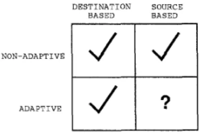
DESTINATION SOURCE

t I

BASED BASED

NON-ADAPTIVE

1

J

1

J

Figure

1:

Routing Methods

route in the packet header. Thus another way of clas- sifying routing is source-based or destination-based ac- cording to the method of addressing the destination processor, which results in a method space shown in Fig. 1.

Although many adaptive routing networks have been constructed and proposed t o date, they have all been destination-based adaptive routing networks. This paper presents the first a ttemp t t o combine the source routing and adaptive routing, referred t o as the adaptive source routing (ASR) method. Th e proposed combination has the advantages of bo th methods. T he route and the adaptivity of each packet is determined a t the source processor node. Every packet can be routed in a fully adaptive, or partially adaptive, or oblivious manner, all within the same network a t the same time. The ASR method also provides support for multiple types of network traffic, in-order delivery of multiple packets, and network partitioning.

In the following, we give a n overview of adaptive, destination-based, and source-based routing methods. In Section

2,

we describe the proposed Adaptive Source Routing method. In Section 3, we present a perfor- mance comparison of the ASR networks and the obliv- ious routing networks by simulations. In Section 4, we present a route generation algorithm that finds m a x - i m a l l y adaptive routes between the processor nodes. This algorithm enables the ASR method.

1.1

Background

In

adaptive routing networks, message packets make use of multiple paths between source-destination node

pairs [7]. Switches alleviate congestion by sending packets via less busy alternate routes. Typically, a busy output port will cause a n adaptive routing switch to use another output in routing a packet to its desti- nation. In a (destination-based) adaptive routing net- work, a switch element must therefore “know” which of its outputs lead t o the intended destination. There- fore, a common characteristic of many adaptive rout- ing networks is a regular and simply described network topology such a s a hypercube, mesh, k-ary n-cube, or a fat tree [4, 5, 7, 8, 91. The switches then have an implicit knowledge of the entire network topology, and therefore they can route packets accordingly.

A

disad- vantage of adaptive routing is that it limits the choice of network topologies. In a n alternative approach, each switch may have a routing table t ha t maps destination processor addresses t o the switch port numbers, how- ever this will occupy real-estate on the switch (chips) and the bounded size of the tables may limit scalability of the networks.

In the destination-based routing, the address (e.g. position) of the destination processor in the network, or a n address difference between source and destina- tion, is encoded in the packet header and then the net- work decides how t o route the message. The source processor has no influence on the routing decisions. This method also requires switches to have a global knowledge of the network topology in order to correctly route packets. Some examples of destination-based networks are the CM-5 fat tree [5] and Intel Paragon 2-dimensional mesh [6].

In the source routing method, unlike destination- based routing, switches need not know the topology; the source processor determines the route and encodes the routing instructions in the packet header. Switches then follow these instructions t o forward the packet t o its destination. Cray T3D [3] and IBM SP2 [l] sys- tems are based on source routing networks. For exam- ple, in the SP2 multistage network, which consists of 8 x 8 switches, the packet header initially contains 3-

bit routing words

R I ,

R2,.

. .

,

Rn,

where n is the num- ber of network stages t o travel. Each word indicates a switch port numbered from 0 t o 7. The source proces-

sor determines the route a nd puts respective words in the header. Each switch forwards the packet through the output port indicated in the first route word and strips off the first word before forwarding the packet to the next level in the network [l]. Thus, the packet contains no routing information upon arriving a t its destination. In t h e source routing method, typically routing headers are computed only once a nd then kept in a route table in each processor node. The route ta- ble approach enables faulty links and switches to be

mapped out easily, and allows more choices of network topologies tha.n destination-based routing, and allows multiple routes t o be defined per destination.

2

Architecture

In the adaptive source routing method proposed here, the key idea is in the definition of the routing words in a packet header. Each routing word indi- cates a set of permitted output ports, rather than a specific output port. Each m-bit word has the format

R

= T,-IT,-~.. . T O , where m is the number of switch

ports. One bits in the routing word indicate the set of outputs that the switch is permitted to use for forward- ing the packet. Th e source processor is responsible for encoding the correct routing instructions in the header a s in the source routing method.

Each switch examines the first word of each packet an d (adaptively) selects a n unused port from one of the permitted outputs t o forward the packet t o the next network stage. If none of the permitted ports are available, then the packet will be blocked an d cannot proceed until at least one of the ports become avail- able. The switch strips off the first route word be- fore forwarding the packet as before. For example, in the 32 node network given in Fig. 14, the header of a packet from processor 4 t o 30 may consist of words

R I

= 11110000, R2

=

11110000,

R3

= 10000000,

Re =

01000000. The header indicates t o the first, second, third, and the last stage switches th at they may for- ward the packet through one of four ports 4-7

( R I ) ,

one of four ports 4-7 ( R 2 ) , port 7 (R3), an d port 6

(&),

respectively. In general, the number of distinct paths a packet may follow from source to destination is

where

lRil

is defined as the number of one bits in the routing word I&. Obviously, not only N p a t h paths must exist between the source a nd the destination, but any combination of the outputs specified in the successive routing words in the header must correctly lead the packet to its intended destination.

Each source processor can choose the adaptivity of a message packet by varying Npath. If N p a t h = max, then the adaptivity is maximum a nd packets may reap per- formance benefits of full adaptivity. This case is useful to minimize network contention due t o non-uniform message traffic and difficult communication patterns. If Npath

= 1,

then the routing is oblivious. The packet is to be routed through a single deterministic path. The N p a t h = 1 case may be useful in several ap- plications. If interprocessor communication patterns

are known in advance, such as for permutation rout- ing on SIMD machines, an optimal set of oblivious routes may be selected to minimize contention [ll]. T h e Npath = 1 case is also valuable for avoiding the

over-taking property of adaptive networks. Over- taking means that the successive packets that belong to the same message may arrive a t their destination out of order, which requires the receiving processor to buffer and sort them. Thus, over-taking may result in more hardware resources being used and may offset performance gains due t o adaptive routing. In a possi- ble implementation t ha t guarantees in-order delivery of packets (that belong to the same message), source processors may send the packets of a multiple packet message non-adaptively, i.e. use Npath = 1, whereas

they may send a single packet message adaptively, i.e. use Npath = max, since single packet messages are not subject to over-taking.

If 1

<

Npath

<

max, then each packet is routed

in a partially-adaptive manner, where only a subset of all possible paths is utilized. This case is valuable for network security or partitioning: When the network is to be logically partitioned among multiple parallel tasks so that their respective communications do not overlap in the network, then by using the partially- adaptive routing method each packet may be forced to remain in its partition, however routed adaptively within the partition.

3

Network Performance

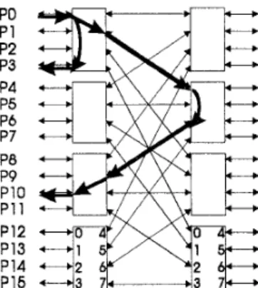
We are primarily interested in the effect of adaptive routing on bidirectional multistage (BMIN) topologies similar to the topologies used in the IBM SP2, the Thinking Machine CM-5 [12], and the Meiko CS-2 [13]. Figure 2 illustrates a 16 processor node BMIN and shows sample routes from a source node 0 t o destina- tion nodes 3 and 10. The 16 ports on the right side are unused in this configuration. The BMIN switches-for this example 8 input, 8 output devices-could be per- mitted t o forward packets from any input port to any output port (including ports on the same “side”).

We have seen few studies directly comparing adap- tive versus oblivious routing for BMIN’s, although the CM-5 machine employs destination-based adaptive routing. In addition, we are interested in assessing the effects of adaptive routing when used in combination with switches t hat incorporate central buffers similar t o SP2 switches [l].

To evaluate the performance of adaptive source routing, we conducted network simulations based upon a

C++

model of SP2-like switches. These switches im- plement buffered wormhoZe routing [1] for flow-control and contain a 1 KB dynamically-shared central buffer.

PO P1 P2 P3 P4 P5 P6 P7 PB P9 P10 P11 P12 P13 P14 P16

Figure 2:

A

16 processor node bidirectional multistage network (BMIN)

Under light to medium loading, a switch is typically able to buffer an entire arriving packet when t hat packet becomes blocked due t o output port contention. Thus, in effect, the switch often operates in virtual cut-through [14] fashion, completely removing blocked packets from network links. However, under heavy loading the central buffer may become full, and pack- ets may then be blocked across several switches, just

as in wormhole routing [15].

In BMIN networks, adaptive choices can typically be made while the packet is traveling “away” from the processors until it reaches any switch which is a least common ancestor of both the source and the destina- tion node. When more than one output port is both idle and permitted for adaptive routing, our simula- tions assume the choice of output port is made on a least-recently-granted basis. The path “back” t o the destination from the least common ancestor switch is unique. We assume minimal paths-if there exists a n h-hop path between source and destination, no

>

h- hop paths may be traversed for communication be- tween them.

All simulations assume an open network model con- taining idealized processor nodes: the nodes contain an infinite transmit queue buffer, and packet flits are immediately pulled from the network as they arrive. We assume a n exponential distribution for message in- jection time (message arrival time). We apply a range of loading to the network, where a load of 1.0 indi- cates that each node is injecting packets in the net- work a t the maximum link d a t a rate. Latency curves include input queueing time and are not shown after saturation (steady-state latency is infinite after satura- tion, assuming infinite input queues). T h e maximum packet size is 255, and messages longer than 255 bytes are broken into multiple packets before transmission.

The open network model makes it possible t o “stress” the network t o a far greater degree and cause

Oblwlous. 4-route -+-

Adaptwe *

100

I

n l -__I

0 0 2 0.4 0.6 0.0 1

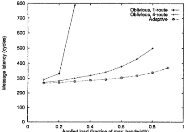
Applied load (fraction of max. bandwidth)

Figure 3: Bit-reversal permutation traffic on a 16-node BMIN topology

more contention t h an might be possible in

a

“real” environment. For instance, in the

SP2,

the processor software a nd the network interface hardware control the injection of message packets via strategies such as end-to-end flow control and message interleaving that significantly reduce the possibility of network cratura- tion and the creation of “hot-spots” [l6]. Therefore the heavily-loaded simulation results shown here are extremely unlikely t o be reproducible in a n actual ma- chine. However, the open network model simplifies analysis by removing the complex software and net- work interface factors, a nd makes it possible to exam- ine a single issue: the effect of adaptive routing.

For each experiment, we compare adaptive routing with oblivious routing schemes. For instance, .in

SP2

systems, each node maintains a route table containing 4 valid minimal routes for each destination node. If there are less t h an 4 unique minimal routes, as when the source an d destination node are connected to the same switch, then 2 or more of these routes are iden- tical. Choosing between 4 routes reduces the effect of contention a n d reduces the probability of creating “hot-spots” in the network.

3.1

Permutation traffic simulation

In this section we investigate the relative per- formance of adaptive routing when the communica- tion pattern is a static permutation. We test 2

permutations: bit-reversal and transpose. In bit- reversal, a source processor represented in binary by sn-1sn-2..

.

slso sends messages t o destination

sosl

..

. s n - 2 s n - 1 . In transposes for even n, the des- tination is SE- SE-2.. . s 1 s o s n - 1 s n - 2 . . .SE+ISE. We

simulate 16-way a n d 64-way BMIN’s. For our simula- tions the 64-way BMIN is constructed from 4 of the 16-way BMIN’s shown in Figure 2. For each 16-way BMIN, the 16 unused right-side bidirectional links are

.

.

.

a a a a 0 hrious. 4-route c Adaptive -+-- 1500 6 6 E

l

p

1000 8

t_

f i ; ...:

i

+ ~ . ~ . ~ ~ + 0 0 0.2 0.4 0.6 0 0

Applied load (fraction of max. bandwidth)

Figure 4: Transpose permutation traffic on a 16-node BMIN topology

connected to a separate switch in a 3rd stage of 16 switches. Thus each 3rd stage switch is connected t o each 16-way BMIN by one link.

Figure 3 displays simulation results for the bit- reversal perrrmtation on a 16-way BMIN topology. Adaptive routing attained both the lowest latency and the highest saturation bandwidth for this difficult per- mutation. For our 1-route oblivious routing, each packet traverses a “straight” path t o a least common ancestor switch, and then the packet proceeds on the unique p ath t’o the destination. This topology has a maximum

of

4

distinct paths between pairs of nodes, and thus 4-ronte oblivious routing is equivalent t o ran- domized routing for the 16-way topology shown in Fig- ure 2. In general, 1-route oblivious routing either per- forms very well or very poorly depending on the per- mutation. Its dismal worst-case performance and high variability make it a poor choice for a general rout- ing strategy, amd we will not consider it further in this paper.

For this 16-way topology, adaptive routing and 4- route oblivious routing have exactly the same paths available. However, with adaptive routing any packets traveling a 3-hop path are guaranteed not t o contend with any other packets while traversing the first switch stage. Why? For this first hop, only 4 input ports (the “left” input ports in Figure 2) are contending for the

4

“right” output ports of the switching element (pack- ets cannot enter and then exit the “right” side of the switching elernent, because the resulting p ath would not be minimal). Therefore if a packet is entering the “left” side, there are

5

3 other input ports currently sending packets to the “right” side, leaving a t least one “right” output port open. The 4-route oblivious pack- ets may often contend in the first stage, an d this is the major cause of higher latency for this experiment.

1400

OblNiouS, 4-route, 100-bvte msas

-

3500

Oblivious, 4-ro te, 100-byte msgs. + Adaptie 1 OO-byte msgs. -+-.

ObiNious, 4-rohte: 500-byte msgs.

Adappe, 500-byte msgs.

-

- - 3000 - I I I 0 0 2 0 4 0 6 O B 1 Applied load (fraction of max bandwidth)

Figure 5: Transpose permutation traffic on a 64-node BMIN topology

0 0 2 0 4 0 6 0 8 1 Applied load (fraction of max ban&idth)

Figure 6: Short message random traffic on a 16-node BMIN topology

mance for the transpose permutation. Again adap- tive routing performs better, and in fact encounters

no contention. The 4-route method loses bandwidth principally because of contention in the first hop.

We have established that adaptive routing performs well for several types of permutation traffic on small systems. We now briefly examine the performance of one permutation on a larger system to illustrate that the benefits of adaptive routing extend over a range of system sizes. Figure 5 displays the latency curves for the transpose permutation on a 64-way BMIN topol- ogy. Adaptive routing still obtains lower latency and higher saturation throughput, although it no longer achieves the “no contention’’ curve of the 16-way sys- tem. For the 64-way system, packets with source and destination in different 16-way groups will traverse 5 switches and have 16 possible least common ancestors. Thus, 4-route oblivious routing no longer corresponds t o random routing, and we include the 16-route obliv- ious case t o demonstrate tha t adaptive routing main- tains performance advantages over random routing as

1200

1

x Adaptive, 1 O O - b ~ e msss. -+--- Oblpious. 4-route. 500-byte m s g s -e---

,

Adaptive, 500-byte m s g s -*

n l I

0 0 2 0 4 0 6 O B 1

Applied load (fraction of max bandwidth)

Figure 7: Short message random traffic on a 128-node BMIN topology

a000

x Oblivious, 4-route, ZOOO-byte Adaptive. 2OOO-byte msgs. msgs.

-

-+--- p ,’ Oblivious, 4-route. EOOO-byte m s g s . -e---

Adaptive, BOOO-byte msgs. -*. .

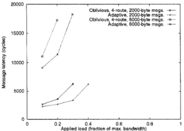
0 0 2 0 4 0 6 0 8 1

Applied load (fraction of max bandwidth)

Figure 8: Long message random traffic on a 128-node BMIN topology

the system size grows. Other permutations and system sizes support similar conclusions, but we will not ex- haustively detail results to further support these claims here.

3.2

Random traffic simulation

In other experiments, we injected traffic with a uni- form destination distribution: for each message, the source randomly chooses any node except itself as the destination. Figure 6 plots message latency for adap- tive routing and 4-route oblivious routing for short (100-byte and 500-byte) messages. Latency before sat- uration is lower and saturation load is higher for adap- tive routing, although neither criteria is significantly better than that of oblivious routing.

To see how the effect of adaptive routing for ran- dom traffic changes with system size, Figure

7

shows the results of the same short message experiment con- ducted on a 128-way BMIN, a n example of which can be found in [l]. For this larger topology, the positive ef- fects of adaptive routing on random routing are more

pronounced. There are more stages in which. adap- tive routing avoids contention compared with oblivious routing.

Figure 8 shows the results of the same 128-way ex- periment conducted with longer (2000-byte and 8000- routing saturates the network a t a 25% highe.c input load t h an 4-route oblivious routing. As messages be-

GENERATE-ltOUTES( GT, 9)

G,,

~-

BF91(GT,

2 for each processor d

#

s do 3 GR t BFSZ(G,,, d ) ;

4

Gs +- AIJL_FEASIBLE-ROUTES(GR);

6 return the routing table RT

Figure 9: Generating routes from a processor t o other byte) messages. For the longer messages, adaptive 5 RT,d t IklAXADAPTIVEROUTE(Gs);

-

-

come longer, the effect of hot-spots becomes greater, and adaptive routing tends to shift traffic awa.y from heavily loaded parts of the BMIN network.

To summarize: for BMIN’s, adaptive routing is gen- erally superior t o oblivious routing for both permuta- tion an d random routing. The advantages accrue for two reasons:

(1)

Adaptive routing does not contribute t o contention on the path “away” from the processors, because for this portion of the path each packet al- ways finds a n output port link available.

(2)

Even in the absence of contention, adaptive routing random- izes traffic by choosing among several available output ports going “away” from the nodes.

4

Routing Algorithm

In this section, we describe a n algorithm that, gener- ates the adaptive routing headers of the message pack- ets. T h e algorithm maximizes the adaptivity, (Npath),

of the header. The problem of maximizing the adap- tivity may be complicated by irregularities in the net- work topology, such a s faulty links and switches. Here, we present a n approach that is applicable t o any multi- stage interconnection network, including networks with faults and partitioned networks.

We represent the topology of the network by a di- rected graph

GT

=

(VT,

E T ) ,

which is referred here as the topology graph. The vertex set

VT

contains two types of nodes, namely processor nodes and switching nodes. T h e edge set ET represents the interconnections between the switching nodes a nd between the proces- sor an d switching nodes. Each edge e

=<

U , v

>

has an

m-bit binary label &[e] whose 1-bit position denotes the output port number of the switching vertex U it is

sourced from. For the sake of efficiency, multiplie edges between the same pair of vertices in the same djirection are coalesced into a single edge. The label of the coa- lesced edge is obtained by bitwise OR’ing the labels of the individual edges.

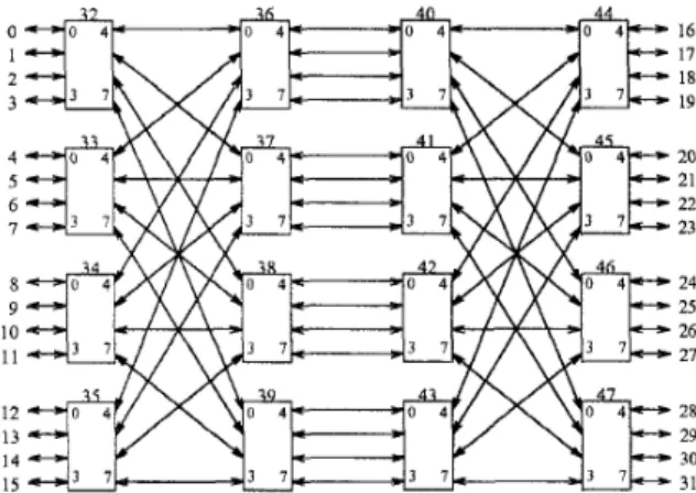
We will work out a n example on a 32 node network shown in Fig. 14. The topology graph

GT

= ( ~ V T ,

E T ) contains 48 vertices which represent the switching nodes an d processor nodes. The processors are indexed from 0 t o 31 and switches are indexed from 32 to 47. In the examples t o follow, the message source will be processor 4 and its destination will be processor 30.

processors

Each processor node, s E

VT,

calls the GENER-

ATE..ROUTES(GT,S) function given in Fig. 9 to deter- mine the set of adaptive routes from itself t o every other processlor d E

VT

in the network. The first step (line 3) of the function finds all possible shortest paths from source t o the destination processor on a routabil- i t y g m p h . The second step (line 4) enumerates all feasi- ble adaptive routing solutions on a s o l u t i o n graph. T he last step (line

5)

selects a route from the solution graph with the maximum adaptivity and stores the result in the routing table.

4.1

Routability

Graph

A

routability graph G R =

(VR,

E R ) enumerates all possible shoriest paths from a source t o a destination processor.

A

routability graph contains only switch- ing nodes and it is a subgraph of the topology graph with all switching nodes an d edges th at are not in the shortest paths from the source t o destination node eliminated. For example, Fig. 15 shows the routabil- ity graph for the source-destination pair (4,30) of the network given in Fig. 14. Usable output ports are in- dicated by the edge labels.

Formally,

GR

=

(VR,ER)

for a given source- destination processor pair is defined to be a directed n-stage multistage graph [17], where a denotes the shortest path distance between the source and desti- nation processors. Here, distance refers to the number of switching elements in a route. Each vertex v E VR has an m-bit binary attribute portsR[W] whose 1-bit positions denote the output ports allowed during rout- ing t o reach idhe destination processor. Vertices

V i

a t each stage

i

are indexed in decimal ordering from 0 to - 1, for

i

= 1 , 2

,...,

a. Both first and last stages contain a single vertex v i and

vg

which corre- spond to the source an d destination switches, respec- tively. Here, source and destination switches refer to the unique switching nodes to which the source and the destination processors are connected, respectively. T he routing word

R,

for reaching the destination processor from the the destination switch is known in advance. Edges exist only between the vertices of the succes- sive stages. T h a t is,

<

u , v > E E R only if U E

V i

an d

v

E

Vi+‘

for some

i

= 1,2,.

. .

,

n

-

1. Each edge

B F S ~ ( G T

,

S)

1 for each vertex 21 E VT

-

{s} do 2 color[v] t WHITE;

3 color[s] t GRAY; depth[s] t 0 ; Q t {s};

4 while Q

# 0

do

5 U +- head[&];

6 for each w E A d j ~ [ a ] do 7

8 color[v] t GRAY; depth[v] t depth[%]

+

1; 9 10 FIFOENQUEUE(Q, U); 11 12 14 r e t u r n G,, = (V,,, E,,), where if COZOT[V] = WHITE t h e n .[VI +- { U } ;

e,,[<

w , U

>]

+ !T[< U , v

>];

elseif color[v] = GRAY a n d

depth[v] = depth[u]

+

1 t h e n

.[.I

t 4 2 1 1 U { U } ;

e,,

[< 21, U

>]

+

e,[<

U , 2,

>]

13 FIFODEQUEUE(&); coloT[U] +- BLACK

v,,

= {'U E VT : cOlOr[v] = BLACK } - {s} E,, = {< u,w >: U , V E Vw, and w E .[U]} Figure 10: T h e BFS-like algorithm proposed to con- struct the predecessors subgraph GT,

=

(VTs

,

ET,)

for the source processors.

e

=<

U , v

>

is labeled with !,[e] similar to

GT.

T h e routability graph for a given source-destination processor pair ( s , d ) is constructed in two steps. In the first step, we use a modified Breadth-First-Search (BFS) algorithm on GT starting from the source ver- tex s. T he proposed BFS-like algorithm-BFS1(GT, s)

in Fig. 10-constructs the predecessors subgraph GT, =

(V,$

,

E T S ) which is different from the breadth-first tree generated during conventional BFS [18]. In G T s , V,, contains all processor nodes of

G T ,

a nd those switching nodes of

GT

which are in the shortest route from the source processor s t o a t least one destination proces- sor other t h a n s. Similarly,

ET*

contains those edges (links) of GT in reverse direction which are in the short- est route from the source processor s to a t least one destination processor other than s. As seen in Fig. 10, each node v E VTS contains multiple parents stored in its 7r,[v] field which also denotes the adjacency list of vertex v in GT,. Hence, edge list E T , of GT, is con- structed on GT in adjacency list format by the T fields

of the vertices in

V,,.

In the second step, the routability graph for a processor pair ( s , d ) can easily be constructed by running another BFS-like algorithm--BFS2(GT,, d ) in Fig. 11-on G,, starting from destination processor d. In Fig. 11, each non-black (white and gray) vertex v E V,, encountered while scanning the adjacency list of a vertex U of depth j from the destination switch

constitutes a n edge from vertex v to U at stages i a nd

i

+

1 of GR, respectively, where i

=

n

-

j - 1.

4.2

Solution Graph

A

solution g r a p h Gs =

(VS,

E s )

enumerates every feasible adaptive route solution (route-word encoding)

BFSZ(G,,, d )

1 dsw t ~ [ d ] ;

2 for each vertex w E V,, - { d s w } do

3 color[v] t WHITE;

5 while Q

# 0

do

6 U t head[Q]; 7 for each w E .[a] d o 8

9 color[v] t GRAY; A d j ~ [ v ] t { U } ;

10

11

FIFOENQUEUE(Q,V);

/*

d s w is the destination switch

*/

4 co~o?'[d8w] t GRAY; Q t { d s w } ;

if color[v] = WHITE t h e n p o r t s R [ v ] + L,,

[<

'11, 2,

>I;

s t a g e ~ [ v ] t depth,, [w];

1 2 else

/*

color[v] should be GRAY

*/

13 A d j ~ [ v ] +- A d j ~ [ v ] U { U } ;

/*

"V":

bitwise OR

*/

14 p O T t S R [ w ] +- pOrtsR['J]

v

&,[< U ,

>I;

15

17 r e t u r n G R = (VR, E R ) , where

e,[<

V , U >] +-

e,,

[< U , 21

>];

1 6 FIFOENQUEUE(Q); COlO?'[U] t BLACK VR = {'U E

v,,

: CO~or[v] = BLACK }

E R = {< U , V

>:

U , V E VR and v E A ~ ~ R [ u ] }

Figure 11: The BFS-like algorithm proposed t o con- struct the routability graph

GR =

( V R , E R )

for the source destination pair ( 5 , d).

from a given source t o a given destination. Formally, G s = (VS, E s ) is defined to be a multistage graph with the same number of stages as in the routability graph GR. The vertex set

V i

of G s at stage

i

is a subset of the power set of V i of G R excluding the empty set, i.e.,

V i

2vA

-

0.

It

is clear that both first and last stages (stages

1

and

n )

of Gs contain a single vertex

v:

and U? which correspond t o the source and destination

switches, respectively.

In a straightforward implementation, we allocate

21vil

-

1 vertices for constructing the stage

i vertices

of Gs. Allocated vertices of each stage are indexed in decimal ordering starting from 1 t o 21vgl - 1. The positions of the 1-bits in the binary representation of each vertex

vi

E V i determine the subset Sf of ver- tices (switches) a t stage i of GR t h a t it represents. For example, a t stage 2 of the routability graph shown in Fig. 15, there are 4 vertices 0, 1, 2, 3 corresponding to switches 36, 37, 38, 39, respectively. Therefore, at stage 2 of the corresponding solution graph shown in Fig. 16, there are 24 - 1

=

15 vertices labeled in binary 0001 through 1111, representing all possible subsets of the set of

4

vertices in the routability graph. As is also seen in Fig. 16, v:3 E

V i

of G s represents the ver- tex subset Sf3 = {si, s ; , si} = {36,38,39} of V i since 13

=

"1101" in binary.

A

vertex

vi

E

V i

only if there exists a t least one feasible adaptive route

R1R2..

. R,

which can forward the message initiated from the source processor t o ex- actly one of the switches in Si through

RlR2..

. R,-1.

Here, feasibility refers to the fact that the remaining n -

i route words

&&+I..

.R, can forward the mes-

sage packets at all switches in Si to the destination processor. An edge e

=<

v f , vi" > E Es only .if there exists at least one feasible route whose stage-i :routing word

R;

forwards the message packets at all switches in

Si t o exactly one of the switches in S:+'. Each edge e is associated with a label &[e] which corresponds to the maximal routing word which achieves the above men- tioned message forwarding. Here, maximality rlefers t o the routing word with maximumnumber of 1's. Hence, the sequence of labels (routing words) on the edges of each distinct path from

vi

t o w y constitutes a :feasible route from the source switch t o the destination switch. Each one of these feasible routes appended with the pre-determined routing word

R,

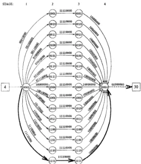
from the destination switch to the destination processor constitutes a fea- sible adaptive route from the source processor t o the destination processor.

For example, in Fig. 16, the vertex vg

=

0101 a t stage 2 has an outgoing edge with the label 11.110000 to the vertex vg = 0101. This edge indicates that from the set of switches Si

=

{sg,s;}

=

(36,38} at stage 2 of

G R ,

we can reach the set of switches

St

=

{sg, s;} = {40,42} at stage 3 of

GR

by the rout- ing word 11110000 which can be verified from Fig. 15. So, the set of switches reached from the switch set {36,38} by the routing word 11110000 is the union of the sets reached from all members.

Fig. 12 illustrates the pseudo-code of the algorithm for creating the solution graph. The first outer for-loop (lines 1-5) and statement at line 6 perform the neces- sary initializations. Here, InAdj and OutAdj denote the adjacency lists of the vertices for their incoming and outgoing edges in

Gs,

respectively.

The second outer for-loop (lines 7-21) performs a forward pass over the vertex stages starting from the only active vertex v i a t stage 1 which corresponds t o the source switch. In this for-loop, only active vertices are processed a t each stage i to determine the active vertices a t the following stage i + l and create the edges between the active vertices a t stages i and i

+-

1. At line 9, Pa is a n m-bit binary number whose 1-bit posi- tions correspond to the common ports of the switches in Sa which can be used t o reach the destination.

In

the for-loop at lines 10-21, all possible route words cor- responding t o the 1-bit positions of Pa are enumerated and processed. For a Pa with 1

5

IC

5

m 1-bits, 2 k - 1 route words are generated 'by fixing the bit positions corresponding t o the 0-bit positions of

Pa

t o all 0's and enumerating 2 k - 1 distinct non-zero binary numbers

from 1 to 2 k - 1 on the bit positions corresponding t o the 1-bit positions of

Pa.

The set Si+'

C

V

i

'

'

R

ALL_FEASIBI;EROUTES( GR)

1 for i +- 1 to n do

2 allocate IVil = 21vil - 1 nodes

{'U;}C'

for V i 3 for j t I., to IVil do

4 m a ~ k [ v ; ] f - INACTIVE; 5 6 marlc[v:] t- ACTIVE; 7 f o r i c l t o n - 1 d o 8 9 pa + / \ u ~ ~ , ?"JTtsR[u]; 10 InAdj[uj] t

0;

OutAdj[vj] t

0;

for each ACTIVE vertex a E VG do

/*

"A"

: bitwise AND operation

*/

for each possible routing word R; E

(1-bit position combinations of

Pa}

d o

for coach stage-i vertex U E Sa of V i do 11 $1 t

0;

14 t

szi

U {w};

12

13 for each w E A d j ~ [ u ] such that

&R[< U , w >]

A

Ri

#

0 do

15 find the vertex 'U E

Vit1

where

S,

= S g ' ;

16 if 'U

fi!

OutAdj[a] then

17 mark[v] t ACTIVE;

18 O ~ t A d j [ a ] t OutAdj[a] U {v}; InA4dj[v] t InAdj[v] U { a } ; 19 l s [ < U , V

>J Ri;

20 else

/*

edge

<

a , v

>

already exists

*/

21

e,[<

a , ' ~

> ]

is[< a l v

> ]

V

Ri;

/*

"v"

: bitwise OR operation

*/

22 for i t n -- 1 downto 2 do 23 24 25 26 27 28 re tu rn G S =

(VS,

Es), where

for each ACTIVE vertex a E

vi

do

for each U E InAdj[a] do

if OutAdj[a] =

0

t h e n

remove vertex a from OutAdj[u];

/*

remove edge

<

U , a

> */

InAclj[a] t

0;

marh[a] t INACTIVE;

vs = {'U : m a T k [ v ] = ACTIVE }

Es =

{<

U , 'U

>:

U , 'U E Vs and 'U E OutAdj[u]}

Figure 12: The algorithm for generating the solution graph Gs = i(Vs, E s )

of switches reached from the switch set

Sa

C

V i

by the routing word R, is constructed in the for-loop at lines 12-14. 'The search operation at line 15 can be ef- ficiently performed in constant time by exploiting the proposed vertex encoding in

GR

and Gs. The if-clause at lines 16-19, adds the edge e

=<

u , v

>

t o E s , ac- tivates vertex v at stage i

+

1 of Gs, and initializes the route-word label &[e] of edge e . The else clause a t lines 20-21 ensures the maximality of the route-word label 1s [ e ] .

The solution graph

G s

generated

at

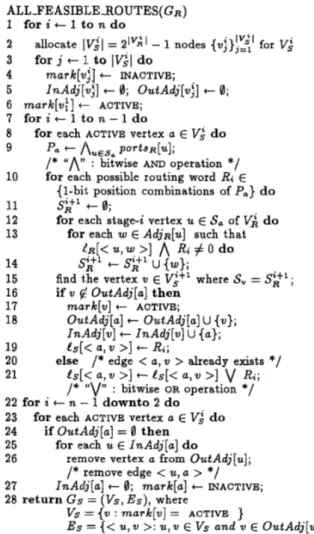
the end of the second outer for-loop (lines 7-21) may cuntain vertices and edges which are not involved in any feasible solu- tion path from the source t o the destination because of the vertices at later stages which do not have any outgoing edges. These infeasible vertices and edges are removed in the last outer for-loop (lines 22-27) in or- der to reduce the computational complexity of the dy-

M A X A D A P T I V E R O U T E ( G s )

1 ADP[wr] t 1;

2 for i c n - 1 downto 1 do

3 for each vertex U E

Vi

do

4 ADP[U] +- 0; 5 6 7 9 nezt[u] +- v ; 11 for i t 1 t o n - 1 do 1 2 v t nezt[u]; 13 R; t is[< U , V >]; 14 U t w ; 15 R, t is[< v f , d >]; 16 return R =

Figure 13: Algorithm for determining maximum adap- tive route in a n n-stage solution graph Gs =

(Vs,

Es). namic programming algorithm to be executed in the next phase. T h e backward processing order over the vertex stages of G s ensures the feasibility of all remain- ing vertices and edges.

for each v E QutAdj[u] do

adp t lis[< U , v

>]I

x ADP[v];

if adp

>

ADP[a] then

8 ADP[.LL] t a d p ;

1 0 U +- v:;

/*

d : destination processor

*/

. . .

R,-iR, with N p s t h = ADP[V:]

4.3

Maximizing Adaptivity

Once the solution graph is created, the maximally adaptive route may be found by finding a path from source to destination node in the solution graph that maximizes the product of the adaptivity values of edges. The adaptivity of a n edge e E Es is defined as the num- ber of 1-bits (i.e., l&[e]l) in its edge label & [ e ] , repre- senting the number of common output port choices of the switches in

Sa

that can be used t o lead the messages a t those switches t o the destination. The adaptivity of a path from source t o destination is the multiplication of the adaptivity values of edges on the path. Hence, the problem reduces t o finding an optimal path from w: to v;" in

G s

with maximumadaptivity. As a n example, in Fig. 16, the top most path has a product cost (adap- tivity) of 1 x

4

x 1

= 4 (i.e.,

1OOOIOOOO/ x ~ 1 1 1 l O O O O ~

x

~ 100 0 000 0 ~), which indicates tha t the given sequence of routing words result in 4 different routes between source and destination processors. Likewise, the bot- tom most path has a product cost of 4 x 4 x 1 = 16 (i.e., ~11110000/ x j11110000/ x ~ 1 0 0 0 0 0 0 0 ~ ) , which shows that the given sequence of routing words result in 16 differ- ent routes between source and destination processors. Note that the bottom most path happens to be the so- lution with the maximum adaptivity; there are no more than 16 distinct shortest paths from processor 4 to 30, as can be verified from Figs. 14 and 15. Therefore, the route header encoding with the maximum adaptivity is

R I

= 11110000, Ra

=

11110000, R3 = 10000000, and Rq = 01000000 in this example. 1 17 2 18 3 19 4 20 5 21 6 22 7 23 8 24 9 25 10 26 11 27 12 28 13 29 14 30 31 15

Figure 14: A 32 processor node bidirectional multi- stage network (BMIN)

A

dynamic programming

[17,

181 formulation for a n n-stage solution graph Gs is obtained by first noticing that every source t o destination path is a result of a sequence of n - 2 decisions. The i-th decision involves

determining which vertex in

V j (1

<

i

<

n) is t o be on a n optimal path.

Let ADP [W;] denotes the adaptivity of the optimal path p ( v i , wy) from the stage-i vertex v$ E Vj t o the destination switch v;". Then, the optimal substructure property gives the recursive formulation

Since the adaptivity of the optimal path from desti- nation switch w;" to the destination processor is 1, the adaptivity of optimal routes from all vertices of G s can easily be computed by performing a backward pass over the vertex stages of G s as shown in Fig. 13. ADP[v:]

contains the adaptivity value of the optimal routing so-

lution(s) when the first for-loop (lines 2-9) terminates. In this for-loop, nezt attribute for each vertex is com- puted to enable the construction of a n optimal routing in the second outer for-loop (lines 11-14). This for-loop constructs a n optimal routing by simply following the next fields of the vertices in forward direction starting from the source switch a t stage 1.

5

Conclusion

In this paper, we presented the first attempt t o com- bine the source routing and adaptive routing meth- ods, referred to as the adaptive source routing (ASR) method. We showed th at the route and the adaptivity of message packets are determined at the source proces- sor node, and tha t packets can be routed in a fully

STAGE: 1 2 3 4

nionnim

. . .

Figure 15: T h e routability graph

GR =

(VR,&R) for the processor pair (4,30).

STAGE: 1 2 3 4

Figure 16: T h e solution graph Gs

=

(VS,

E s )

for the processor pair (4,30).

adaptive, or partially adaptive, or oblivious manner in the same network, at the same time. We described how the ASR method may support multiple types of network traffic, in-order delivery of multiple packets to avoid over-taking, and network partitioning. T h e source routing nature of the ASR method e1i:minates the need for routing tables on the switch chips which may limit scalability and occupy valuable real-estate on silicon. We presented performance comparison of adaptive versus oblivious routing networks. We found adaptive routing t o be generally superior to oblivi- ous routing for both permutation and randomi traffic. We presented an algorithm that generates maximally adaptive routing headers for the message packets. Th e algorithm is applicable t o multistage networks in gen- eral, including faulty networks and irregular topologies.

Acknowledgements:

We are thankful to Mike Rosenfield and anonymous reviewers for their helpful comments.

References

[l] C. B. Stunkel, D. G. Shea, and B. Abali et al., “The sP2 high-performance switch,” I B M S y s t e m s Journal, vol. 34, no. 2, pp. 185-204, 1995.

[2] Cray Research Inc., cray T3D System Architecture Overview, 1993.

[3] S. Scott and G. Thorson, “Optimized Routing in the Cray T3D,” Lecture Notes in Computer Science, Springer-Verlag, vol. 853, pp. 281-294, 1994. [4] C. E. Leiserson, “Fat-trees: Universal networks for

hardware-efficient supercomputing,” I E E E Trans. on Computers, vol. C-34, pp. 892-901, Oct. 1985. [5] Thinking Machines Corporation, Connection Machine

CM-5 Technical Summary, November 1993.

[6] Intel Cor:poration, Paragon

xP/s

Product Overview, 1991.

[7] S. A. Felperin, L. Gravano, G. D. Pifarre, and L. C. Sanz, “Routing techniques for massively parallel com- munication,” Proc. I E E E , vol. 79, pp. 488-503, April 1991.

[8] S. Konstetntinidou and L. Snyder, “Chaos router: ar- chitecture and performance,” in Proc. 18th A n n . Int. Symp. o n Computer Architecture, pp. 212-221, 1991. [9] R. V. Boppana and S. Chalasani, “A comparison of

adaptive ,wormhole routing algorithms,” in PTOC. 20th. Ann. Int. Symp. on Computer Architecture, pp. 351- 360, May 1993.

[lo] C. B. Stunkel, D. G. Shea, B. Abali, M. M. Den- neau, P. H. Hochschild, D. J. Joseph, B. J . Nathanson, M. Tsao, and P. R. Varker, “Architecture and imple- mentation of Vulcan,” in Proc. 8th Int. Parallel Pro- cessing Symp., pp. 268-274, April 1994.

[ll] B. Ab& and C. Aykanat, “Routing Algorithms for IBM SP1,” Lecture Notes i n Computer Science, Springer-Verlag, vol. 853, pp. 161-175, 1994. [12] C. E. Leiserson, Z. S. Abuhamdeh, D. C. Douglas,

C. R. Feynman, M.

N.

Ganmukhi, J. V. Hill, W. D. Hillis, B. C. Kuszmaul, M. A. St. Pierre, D. S. Wells, M. C. Wong, S.-W. Yang, and R. Zak, “The net- work architecture of the Connection Machine CM-5,” in Proc. I1992 Symp. Parallel Algorithms and Architec- tures, pp. 272-285, ACM, 1992.

[13] J. Beecroft, M. Homewood, and M. McLaren, “Meiko CS-2 interconnect Elan-Elite design,” Parallel Com- [14] P. Kermani and L. Kleinrock, “Virtual cut-through: A new com:puter communications switching technique,” Computer Networks, vol. 3, pp. 267-286, Sept. 1979. [15] W. J. Dally, “Performance analysis of k-ary n-cube in-

terconnection networks,” I E E E Trans. on Computers, vol. 39, pp. 775-785, June 1990.

[16] M. Snir, P. Hochschild, D. D. Frye, and K . J. Gildea, “The communication software and parallel environ- ment of the IBM SP2,” I B M Systems Journal, vol. 34, no. 2, pp. 205-221, 1995.

[17] E. Horowitz and S. Sahni, Fundamentals of Computer

Algorithms. Maryland: Computer Science Press, 1989. [18] T. H. Cormen, C. E. Leiserson, and R. L. Rivest, In- troduction to Algorithms. NY: The MIT Press, 1991. puting, vol. 20, pp. 1627-1638, NOV. 1994.