On the measurement of productivity and environmental efficiency in the presence of the joint production of goods and bads : an application to OECD countries

(1)

(2)

ON THE MEASUREMENT OF PRODUCTIVITY AND ENVIRONMENTAL EFFICIENCY IN THE PRESENCE OF THE JOINT PRODUCTION OF

GOODS AND BADS:

AN APPLICATION TO OECD COUNTRIES

The Institute of Economics and Social Sciences of

Bilkent University by

Barış K. Yörük

In Partial Fulfillment of the Requirements for the Degree of

MASTER OF ARTS IN ECONOMICS in

THE DEPARTMENT OF ECONOMICS BİLKENT UNIVERSITY

ANKARA July 2003

(3)

I certify that I have read this thesis and have found that it is fully adequate, in scope and quality, as a thesis for the degree of Master of Arts in Economics. ---

Assoc. Prof. Dr. Osman Zaim Supervisor

Assoc. Prof. Dr. Syed Fakhre Mahmud Examining Committee Member

Assist. Prof. Dr. Süheyla Özyıldırım Examining Committee Member

Approval of the Institute of Economics and Social Sciences ---

Prof. Dr. Kürşat Aydoğan Director

(4)

iii

ABSTRACT

ON THE MEASUREMENT OF PRODUCTIVITY AND

ENVIRONMENTAL EFFICIENCY IN THE PRESENCE OF THE JOINT PRODUCTION OF GOODS AND BADS: AN APPLICATION TO OECD

COUNTRIES Yörük, Barış K.

M.A., Department of Economics Supervisor: Assoc. Prof. Dr. Osman Zaim

July 2003

Productivity measures, which do not account for environmental performance, are biased. When it comes to incorporating the developments in environmental performance into the measurement of productivity, the traditional “Tornquist type” indices fail to measure the productivity particularly in the cases where price information on undesirable outputs do not exist. Therefore, there is a need for an alternative measure which puts due emphasis on production with negative externalities without requiring price information. Motivated by these facts, this study first employs a Malmquist index for OECD countries without considering the existence of pollutant data and then to overcome the shortfall of this index, a Malmquist-Luenberger productivity index is employed. Furthermore, using an index number approach, environmental performance of OECD countries is also evaluated, by using a method, which relies on the computation of the distance functions within a DEA framework.

Keywords: environmental efficiency index, index numbers, Malmquist productivity index, Malmquist-Luenberger productivity index, OECD countries

(5)

iv

ÖZET

FAYDALI VE ZARARLI MADDELERİN BİRLİKTE ÜRETİMİNDE VERİMLİLİK VE ÇEVRESEL PERFORMANSIN ÖLÇÜMÜ ÜZERİNE:

OECD ÜLKELERİ ÜZERİNE BİR UYGULAMA

Yörük, Barış K. Yüksek Lisans, İktisat Bölümü Tez Yöneticisi: Doç. Dr. Osman Zaim

Temmuz, 2003

Çevresel performansı dikkate almayan verimlilik ölçüleri hatalı sonuçlar vermektedir. Çevresel performansı verimliliğe dahil etmeye çalışan klasik “Tornquist” tipi indeksler de zararlı maddelerin fiyat bilgisinin bilinmediği durumlarda verimliliği ölçememektedir. Bu yüzden, fiyat bilgisine gerek duymayan ve zararlı maddelerin üretim sürecinde olduğu durumlarda kullanılabilecek alternatif ölçülere ihtiyaç duyulmaktadır. Bu noktadan hareketle, bu çalışma verimlilik ölçümünde öncelikle OECD ülkeleri için zaralı maddelerin üretim sürecinde var olduğunu dikkate almaksızın Malmquist indeksi kullanır. Daha sonra bu indeksin eksik yönleri göz önünde tutularak Malmquist-Luenberger üretim indeksi kullanılmıştır. Ayrıca OECD ülkelerinin çevresel performansı DEA metodu çerçevesinde uzaklık fonksiyonlarının hesaplanmasına dayanan indeks rakamları yaklaşımıyla ölçülmüştür.

Anahtar Kelimeler: çevresel verimlilik indeksi, indeks rakamları, Malmquist verimlilik indeksi, Malmquist-Luenberger verimlilik indeksi, OECD ülkeleri

(6)

v

ACKNOWLEDGEMENTS

That’s my honor to express my gratitude to Associate Prof. Dr. Osman Zaim for his supervision and guidance throughout the development of this thesis. I would like to thank Assoc. Prof. Dr. Syed Mahmud, Assist. Prof. Dr. Süheyla Özyıldırım and Tümer Kapan for their valuable comments.

I am grateful to my family for their support and understanding during my whole life.

(7)

vi

LIST OF TABLES

4.1.1. The Data as the Average of the Period 1983-1998……….28

4.2.1. Malmquist Productivity Index and Decomposition: 1985-1998………….30

4.2.2. Malmquist-Luenberger Indices and Decompositions: 1985-1998………..32

4.2.3. Malmquist Productivity Index……….60

4.2.4. Malmquist Productivity Index (Efficiency Change)………...61

4.2.5. Malmquist Productivity Change (Technical Change)……….62

4.2.6. Malmquist-Luenberger Productivity index, Bads: CO2………..63

4.2.7. Malmquist-Luenberger Productivity index, Bads: CO2 (Eff.)……….64

4.2.8. Malmquist-Luenberger Productivity index, Bads: CO2 (Tech.)………….65

4.2.9. Malmquist-Luenberger Productivity index, Bads: NOX and CO2………..66

4.2.10. Malmquist-Luenberger Productivity index, Bads: NOX and CO2 (Eff.)...67

4.2.11. Malmquist-Luenberger Productivity index, Bads: NOX and CO2 (Tech.) ………...………...68

4.2.12. Malmquist-Luenberger Productivity index, Bads: NOX and Organic Water Pollutant ………...69

4.2.13. Malmquist-Luenberger Productivity index, Bads: NOX and Organic Water Pollutant (Eff.)………...70

4.2.14. Malmquist-Luenberger Productivity index, Bads: NOX and Organic Water Pollutant (Tech.)………71

4.2.15. Malmquist-Luenberger Productivity index, Bads: CO2 and Organic Water Pollutant ………..…….72

(10)

ix

4.2.16. Malmquist-Luenberger Productivity index, Bads: CO2 and Organic Water

Pollutant (Eff.)………..………73

4.2.17. Malmquist-Luenberger Productivity index, Bads: CO2 and Organic Water Pollutant (Tech.)………..……….74

4.3.1. Spearman Correlations of Indices……….……….33

4.4.1. Environmental Performance of OECD Countries……….……….45

4.4.2. Environmental Quantity Index, Bads: NOX and CO2……….…...76

4.4.3. Environmental Performance Index, Bads: NOX and CO2………….……77

4.4.4. Environmental Quantity Index, Bads: NOX and Organic Water P….…...78

4.4.5. Environmental Performance Index, Bads: NOX and Organic Water P…..79

4.4.6. Environmental Quantity Index, Bads: CO2 and Organic Water P………..80

(11)

x

LIST OF FIGURES

3.1.1. An Output Set………..16

3.2.1. Output-Oriented Malmquist Productivity Index………..20

3.3.1. Distance Functions………...23

4.3.1. The Trend of Pollution Emissions in OECD………...34

4.3.2. The Trend of Indices for OECD……….35

4.3.3. The Trend of Pollution Emissions in Great Britain……….37

4.3.4. The Trend of Indices for Great Britain………38

4.3.5. The Trend of Pollution Emissions in Norway……….39

4.3.6. The Trend of Indices for Norway………40

4.3.7. The Trend of Pollution Emissions in Canada………..41

(12)

1

CHAPTER 1 INTRODUCTION

Since the introduction of famous growth model by Solow (1956, 1957), the accurate measurement of productivity and efficiency has been one of the most important and widely discussed issues of economic literature. The Solow model focuses on four variables namely output, capital, labor and “knowledge” or the “effectiveness of labor”. According to the model, at any time, the economy has some amounts of capital, labor and knowledge and these are used to produce outputs. Then, simply put, we may say that in any production process, for a given inputs, outputs are produced.

Beyond the theory, individual figures or economic variables of countries do not help us to make comparisons or correctly assess the productivity. For this purpose, we have productivity growth measures or indices. In a very simple manner, efficiency and productivity measurement tell us about how well a firm or a country is doing to relative to some benchmark, which is constructed over the whole sample. By this kind of approach and with the help of productivity indices, we are able to judge the performances of countries relative to the whole sample.

Traditional measures of productivity growth have only concentrated on production of desirable outputs (goods) with no consideration on

(13)

2

environmentally hazardous by-products (bads) of the production process. This type of approach typically yields biased measures of productivity growth.

In the light of this fact, recently a substantial literature has emerged to model the productivity growth in the presence of the joint production of goods and bads. One possible approach is to modify the traditional methodology and productivity indices (such as Tornquist and Fisher indices) so as to incorporate the undesirable outputs. However, this requires price information on both desirable and undesirable outputs as well as inputs considered. In this case, a shadow price for each of the pollutants considered should also be computed. For this purpose, shadow prices can be estimated by following Pittman (1983) or Fare et al. (1993).

An alternative approach to measure productivity by incorporating the undesirable outputs is to employ an index that requires information only on quantities. One such index is referred as Malmquist productivity index. However, in the presence of undesirable outputs in production process, this index has to be modified to incorporate negative externalities. Further discussion and explanation of this problem can be seen in Chung et al. (1997). This index is quite popular in the literature and without considering the negative externalities, employed in various studies that use either micro or macro data.

To measure the productivity in the presence of the joint production of goods and bads, Chung et al. (1997) developed a modified version of Malmquist productivity index, which they referred as Malmquist-Luenberger productivity index. This index credits the reduction of undesirable outputs while simultaneously crediting increases in desirable outputs and similar to original Malmquist productivity index, depends on quantities without requiring

(14)

3

information on prices. Therefore, this index is a useful alternative in measuring productivity.

This thesis first computes a Malmquist productivity index to measure the productivity growth of OECD countries without considering the presence of the negative externalities. To overcome the shortcomings of the Malmquist productivity index, a Malmquist-Luenberger productivity index is computed which accounts for the pollutants in the measurement of productivity. Then Malmquist and Malmquist-Luenberger indices are compared in terms of their strengths and weaknesses in measuring the productivity.

Furthermore, following Fare et al. (1999) an alternative index is employed which is used to evaluate the environmental performance of the OECD countries. This index, using index number approach and DEA framework, relies on the computations of distance functions and aimed to be a well-established methodology in evaluating the environmental efficiency of OECD countries. The organization of the thesis is as follows. The next chapter is dedicated to a summary of previous studies that aim to model the productivity in the presence of pollutants and the survey of literature on the topics investigated. Chapter 3 is reserved for the methodology that is used in constructing indices employed in this study. The next chapter provides the information on the data used and the application of this panel data to construct environmental performance and productivity indices. This chapter also dedicated to the comparison of Malmquist and Malmquist-Luenberger productivity indices. Finally chapter 5 concludes.

(15)

4

CHAPTER 2 SURVEY OF THE LITERATURE

The following sub sections summarize the existing literature on the productivity indices that are used in this study as well as the environmental efficiency indices.

2.1. Malmquist Productivity Index

By using the data on outputs and inputs, the methodology of Malmquist productivity index relies on constructing a best practice frontier and then computing the distance of individual observations from the frontier constructed over the whole sample. In contrast to the alternative indices such as Törnquist and Fischer that require information on both the prices and quantities of all inputs and outputs, this index requires information only on quantities.

By following Stan Malmquist’s (1953) quantity index, Caves et al. (1982a, 1982b) introduced two theoretical indices which they named Malmquist input and output productivity indices. In their pioneering study, they compare two input-output vectors to a reference technology using radial input and output scaling, for the input and output productivity indices respectively. Although their paper was influential, the Malmquist productivity index itself was rarely computed until Fare et al. (1989b) showed how this index could be calculated using non-parametric linear programming method. In their study they also

(16)

5

showed that Malmquist productivity index could be decomposed into technological progress and technical efficiency components. Later, Ray and Desli (1995) decomposed the Malmquist productivity index into three components namely technical change, scale efficiency change and efficiency change.

Following these pioneering theoretical studies, great number of empirical literature has emerged. The application of Malmquist productivity index includes public sectors, agriculture, transportation, banking, electric utilities, insurance companies and the country comparisons of productivity. Since there are literally over 200 empirical papers on Mamquist productivity index, we here cite only the path breaking and significant ones.

The first application of the Malmquist productivity index on public sector was Fare et al. (1994b). They compute the index and decompose into technical and efficiency change components for the Swedish hospital sector for the time period 1970 to 1985. Their results indicate a considerable variation in efficiency change among 17 hospitals in their sample and the technical change component showed both progress and regress. Later, Burgess and Wilson (1995) and Magnussen (1994) applied the same methodology to U.S and Norwegian hospital ownership respectively. The application of this index on Turkey’s public enterprise sector was Taskin and Zaim (1995). Their results showed that the growth in the public sector was 14% on average and 37% for the private sector. The major reason for the growth is technical change while there has been a decline in the efficiency component.

The first study that applied the Malmquist productivity index to agricultural sector was Thirtle, Hadley and Townsend (1994). They computed the

(17)

6

based Malmquist indices for agriculture in sub-Saharan countries for the period 1971-1986. They assumed that land, labor and livestock are used to produce aggregate agricultural output. They found that productivity growth is small but generally positive. To cite, other major empirical studies that employed this methodology on agricultural sector was Tauer(1994), Turk, Piesse and Thirtle (1996) and Ferrantino and Ferrier (1996). Tauer (1994) measured the productivity of New York dairy farms. Turk, Piesse and Thirtle (1996) assessed the performance of co-operative and private dairy farms of Slovenia from 1974 to 1990. Ferranino and Ferrier (1996) used the Malmquist index to measure the performance of Indian sugar industry.

Transportation is another industry that the Malmquist productivity index has been used. The significant examples are Starr McMullen and Okuyama (1996), Good and Sickles (1995) and Distexhe and Perelman (1995). Starr McMullen and Okuyama (1996) computed the Malmquist productivity index for U.S motor carriers over the period 1976 and 1990. They found significant technological regress occurring in 1976-1978, 1979-1981 and 1987-1989. Good and Sickles (1995) applied the same methodology to Western European airline carriers. Distexhe and Perelman (1995) measured the productivity among the international airlines.

Employing Malmquist productivity index on banking and financial sector is quite popular. Most of the works analyze the performance of banks within one country and a few make international comparisons. The first significant example was Berg, Forsund and Jansen (1992). They compute the productivity change for Norwegian banks during 1980’s when the banking industry was deregulated. Their results suggest regress in the earlier years and progress in the later years of

(18)

7

sample on average. Other significant empirical works include Tulkens and Malnero (1996), Fukuyama (1995a), Wheelock and Wilson (1994) and Devaney and Weber (1995). Tulkens and Malnero (1996) analyzed the productivity of 663 branches of one bank in Belgium over 11 month period in 1987. Fukuyama (1995) computed the Malmquist productivity index for Japanese banks over the period 1989 to 1991. Wheelock and Wilson (1994) use the Malmquist index to measure productivity of U.S commercial banks from 1984 to 1993. Devaney and Weber (1995) analyzed the productivity for all U.S rural banks for 1990, 1992 and 1993.

Hjalmarsson and Veiderpass (1992) and Forsund and Kittlsen (1994) are two significant examples of empirical work that employed Malmquist productivity index on electric utility industry. Hjalmarsson and Viedepass (1992) used Malmquist index to measure the productivity of 289 Swedish electricity retail distributors during the period from 1970 to 1986. Forsund and Kittelsen (1994) assess the Norwegian electricity distribution system by the data from 1983 and 1989.

The first study that measures the productivity in a insurance sector was Donni and Fecher (1995). They assess and compare the productivity of insurance sectors of 15 OECD countries from 1983 to 1991. Other significant empirical work includes Fukuyama (1995b) and Cummins, Turchetti and Weiss (1995). Fukuyama (1995b) computed the productivity of Japanese life insurance companies over the time period 1988-1993. He concluded that productivity improved during the time period considered mainly due to technical change. Cummins, Turchetti and Weiss (1995) employed the Malmquist productivity index for 94 insurance companies in Italy for the time period 1985-1993.

(19)

8

Perelman (1995), Taskin and Zaim (1995) and Gouyette and Perelman (1995) are the significant empirical works that employ the Malmquist productivity index in country comparison studies. Perelman (1995) provides an international comparison for a sample of OECD countries for the time period 1970-1987. Taskin and Zaim (1996) compute the Malmquist productivity index for a sample of high and low income countries over the 1975-1990 period. They concluded that the countries with low initial per capita income catch up at a faster rate while countries with relatively high per capita income depend more on technological progress for their productivity increases. Gouyette and Perelman (1995) compute the Malmquist indices for a sample of 13 OECD countries for different sub sectors over the 1970-1988 period.

Although Malmquist productivity index has many desirable properties and applications on different sectors, one should modify this index to assess the productivity in the presence of the joint production of desirable and undesirable outputs.

2.2. Malmquist-Luenberger Productivity Index

This index is actually a modified version of Malmquist index and first presented in Chung et al. (1997). They substitute directional distance functions for the output distance functions in the Malmquist index and rename it the Malmquist-Luenberger productivity index. The new index they proposed in this study overcomes the shortcomings of the original Malmquist productivity index. This index allows for the inclusion of undesirable outputs (pollutants) in the measurement of productivity without requiring information on shadow prices. Since the index is computed using a DEA methodology, information concerning

(20)

9

benchmark samples and technical efficiency is also generated for individual observations. In order to illustrate the applicability of this index, they compute the productivity for the Swedish paper and pulp industry. This index again can be decomposed into efficiency change and technological change parts.

Since the literature on this index is very new, there are considerably few studies available that employ this index in the measurement of productivity. One of the significant examples was Fare et al. (2001). They used a Malmquist-Luenberger productivity index to account for both marketed outputs and the output of pollution abatement activities of U.S state manufacturing sectors for 1974-1983. They found that adjusted productivity growth improved for the sample states after 1977, and the states with rapidly growing manufacturing sectors have significantly higher rates of productivity growth than the states with slowly growing manufacturing sectors.

Another study that incorporates the pollutants into the production technology for state manufacturing industries explicitly was Weber and Domazlicky (2001). They apply the Malmquist-Luenberger productivity index to state manufacturing data and the aggregated emissions for 1988-1994. The productivity index that only considers the desirable output and ignores the output of the pollution abatement activities of the manufacturing sector yields a decline in the annual productivity. However, when the productivity index includes both the expansion of the desirable output and the contraction of the undesirable output (pollutant) they find an increase in the state manufacturing productivity.

Malmquist-Luenberger productivity index is certainly an improvement over the traditional measures of productivity growth and Ma1mquist productivity index. However, this index still fails to establish a link between pollution intensities and

(21)

10

productivity growth since it does not allow us to make cross-country and over time comparisons over developments in pollution intensities i.e., bad over good ratios. Within this framework, alternative indices by index number theory and environmental efficiency indices are developed to measure the environmental performance.

2.3. Environmental Efficiency Index and Alternative Indices

The literature on the environmental efficiency indices depends on the literature of `production frontiers` and `Farrell measure of technical efficiency`, which starts with Farrell (1957) and later extensively covered in Shephard (1970), Fare et al. (1985b), (1994a) and Fried et al. (1993). On measuring environmental performance and constructing the efficiency indices, one of the two methodologies are employed. These are stochastic frontier estimation and data envelopment analysis (DEA). Both approaches are quite favorable. For example, Reinhard et al. (1996) used a stochastic frontier approach to construct an environmental efficiency index with micro level data while Ball et al. (1994) and Tyteca (1997) adapted the DEA methodology to measure environmental performance. Later Reinhard (1997) used both approaches to show the pros and cons of two methods.

There are alternative approaches according to the selection of the type of the efficiency measure in the studies that DEA framework is employed. Fare et al. (1986) and (1989c) used radial measures of technical efficiency to compute the desirable output loss, which stems from the reduced disposability of the undesirable outputs. Another example of using radial measure was Fare et al. (1996). They rely on the comparison of two input (output) oriented radial

(22)

11

technical efficiency scores, one accounts for the production of environmentally undesirable outputs and the other which completely ignores the production of pollutants with desirable outputs.

As opposed to radial measure, the alternative efficiency measure is hyperbolic measure of technical efficiency. In their path breaking study Fare et al. (1989a), suggested this methodology. This measure of technical efficiency allows for simultaneous equiproportionate reduction in the undesirable outputs (bads) with an expansion of desirable outputs (goods). The importance of this measure is to compute the opportunity cost of transforming the production process from one where all outputs are strongly disposable to the one, which is characterized by weak disposability of undesirable outputs. Later hyperbolic measure of technical efficiency is employed in constructing environmental efficiency indices in the works of Zaim and Taskin (1999), Zaim and Taskin (2000) and Taskin and Zaim (2000). They employed this measure and environmental efficiency indices to measure the environmental performance of OECD countries and search for a Kuznets curve relationship in environmental efficiency.

On the other hand alternative indices are also quite popular in measuring the environmental performance. These indices are very much like the Malmquist Index, but rather than scaling the full output vector, they scale the desirable and undesirable outputs separately. These indices are first developed in Zaim et al. (2001) and used in the measurement of human well-being. They propose two indices in this study, which they called achievement (quantity index) and improvement indices. The general methodology again depends on micro tools in index number theory, Farrell efficiency measures and DEA methodology. One very significant property of their indices was that they allow for cross country

(23)

12

and overtime comparisons. It also satisfies some desirable properties such as transitivity, time reversal, homogeneity and dimensionality. These desirable properties in index numbers theory were first presented in Fischer (1922). For a detailed discussion of theoretical underpinnings of various index numbers one can refer to Diewert (1979).

Fare et al. (2002) also developed this methodology and later on, Grosskopf et al. (2003) used the same methodology on measuring how efficiently public health expenditures are translated into better health. The application of this methodology to environmental data is again Zaim (2002). Basically his index is defined as the ratio of a good output quantity index and a quantity index of bad or undesirable outputs. Each of the two indices is based on distance functions and DEA methodology is employed. This study measured the environmental performance of state manufacturing through changes in pollution intensities. The studies on measuring productivity in the presence of pollutants and constructing indices to measure environmental performance also effort to relate and search for an environmental Kuznets curve hypothesis, which assumes an inverted U-type relationship between the levels of emissions and income. For further discussion of this issue see Grossman and Kruger (1993), Cropper and Griffith (1994), Selden and Song (1994), Holtz-Eakin and Selden (1995) and Taskin and Zaim (2000).

(24)

13

CHAPTER 3 METHODOLOGY

This chapter of the thesis presents the basic methodology underlying the indices that are used to measure the productivity in the presence of pollutants as one of the outputs in production process. The indices taken into consideration are Malmquist productivity index and Malmquist-Luenberger productivity index. To measure the environmental performance, an alternative index is also presented which employs the index number approach and DEA methodology using a non-parametric approach. A series of papers such as Fare et al. (1989b), Chung et al. (1997) and Fare et al. (1999) are followed for the methodology presented in the proceeding sections.

3.1. Distance Functions and Joint Production of Goods and Bads

Mainly, in a production process for a given inputs, good (desirable) and bad (undesirable or pollutants) outputs are produced. Formally, denote the good

outputs by M

M

1 y R

y

y=( ,..., )∈ + and the bad outputs by b=(b1,...,bI)∈R+I.

Therefore, the output set ( by, )is produced by the input set N N

1 x R

x

x=( ,..., )∈ + .

Then, technology can be described via its output set: (3.1.1) T ={(x,y):xcan produce( y,b)}

(25)

14

In words, for each input vector N

N

1 x R

x

x=( ,..., )∈ + , the technology set includes

all the combinations of good and bad outputs or the output set( by, ), which can be produced by the vector of inputs.

Technology set is also equivalent to output set P(x)or may be represented by the

input set L( by, )such that:

(3.1.2) (x,y,b)∈T ⇔(y,b)∈P(x)⇔ x∈L(y,b)

The weak disposability assumption of output set ( by, )can be modeled as:

(3.1.3) (y,b)∈P(x )and0≤θ ≤1imply (θy,θb)∈P(x)

In words, this assumption implies that given a fixed level of inputs, a reduction in bads is feasible only when the goods are also simultaneously reduced. However, free disposability of good outputs is still maintained. That is good outputs may be reduced without the reduction of the bad outputs. In notation:

(3.1.4) (y,b)∈P(x )andy′≤ yimply (y′,b)∈P(x)

Equations (3.1.3) and (3.1.4) together model the asymmetry between the good and bad outputs where goods are freely disposable while the bads are not. The last assumption is null-jointness, which says that no desirable outputs can be produced without producing any bad outputs. This idea of joint production of good and bad outputs can be modeled as:

(3.1.5) if(y,b)∈P(x )andb=0 then y=0

In figure 3.1.1, we illustrate an example of such a joint output set that satisfies these properties.

(26)

15

Figure 3.1.1. An Output Set

In addition to the assumptions on the joint production of good and bad outputs, we may also impose some restrictions over the output setP(x). To model the

idea that zero inputs yields zero outputs we have: (3.1.6) P(0)={0,0}

On the other hand, we may also assume that given finite inputs, only finite output can be produced. This is in notation:

(3.1.7) P(x)is compact for each _x _RN

+

∈ The final assumption on output set P(x)is:

(3.1.8) _P₍_x₎_⊇_P₍_x'_),_x_≥ _x' (y, b) (y' ,b) P(x) Bad Good

(27)

16

This assumption imposes free disposability of inputs, which essentially implies that if inputs are increased then output does not decrease.

Fallowing Fare et al. (1994a), we may formulate the activity analysis or data envelopment analysis (DEA). We assume that there are Kobservations on inputs and outputs, where k indexes each individual observation such that

(

)

{

xk_,yk_,bk _:k₌1_,...,K

}

_{. By this data we can construct an output set that holds}

for every period and satisfies our previous assumptions. Formally:

(3.1.9) }, ,..., , 0 z , ,..., , , ,..., , , ,..., , : ) , {( ) ( k 1 1 1 K 1 k N 1 n x x z I 1 i b b z M 1 m y y z b y x P K k n kn k K k k ki i K k m km k = ≥ = ≤ = = = ≥ =

∑

= = =

where the non-negative are the intensity variables (weights) assigned to each z_k observation when constructing the production set. The inequality constraint on

the good output M

M

1 y R

y

y=( ,..., )∈ + in (3.1.9) states the assumption of free

disposability, which means that the desirable output can be disposed of without the use of any inputs. If we also consider the production of bad output

I I

1 b R

b

b=( ,..., )∈ + together with the desirable output, we should impose the

weak disposability condition that satisfies the assumption we introduced in (3.1.3) by choosing an equality sign for the relevant constraint. To satisfy the null-jointness introduced before, we restrict the conditions:

(3.1.10)

∑

= = > K k ki i 1 I b 1 , ,..., , 0 and

(28)

17 (3.1.11)

∑

= = > I i ki i K b 1 ,..., 1 , 0 .

The inequality (3.1.10) states that each undesirable or bad output is produced by some individual sample k (firm or county). On the other hand, (3.1.11) implies every k produces at least one bad output. We may further illustrate null-jointness by assuming that each bi = 0, where i = 1,…, I. Then each intensity variable zk in

(3.1.9) will be zero, implying that all the desirable good outputs ym must be zero. Therefore, these two restrictions can be used to determine whether a particular data set satisfies null-jointness of desirable and undesirable outputs. To impose this assumption our application will not include the data that violate the null-jointness.

Further, the non-negativity of intensity variables in (3.1.9) implies that the production technology exhibits constants returns to scale. That is:

(3.1.12) P(λx)=λP(x),λ>0.

3.2. Malmquist Productivity Index

In this section, we present the Malmquist productivity index without considering the joint production of goods and bads. Since our whole analysis depends on the assumption that we have no information on prices, distance functions are our proxies for defining and measuring productivity. The original Malmquist productivity index uses Shephard distance functions to represent the underlying technology (Shephard, 1970). In the presence of only goods (desirable outputs), these output distance functions can be defined as:

(29)

18

This output distance function is complete characterization of technology. For each observation, the output distance functions can be computed by solving the following linear problem for k`:

(3.2.2) K k z N n x z M m y y z st y x D k K k t kn k K k t t km k k t k t t o ,..., 1 0 ,...., 1 x ,...., 1 max )) , ( ( 1 t n k 1 m k 1 , , ' = ≥ = ≤ = ≥ =

∑

= ′ = ′ − ′ θ θ

Taking t = 1,…, T as our time periods, we can define an output oriented Malmquist productivity index that does not incorporate the bad outputs by fallowing Fare et al. (1989b) such that:

(3.2.3) 2 1 1 1 1 1 1 1 1 1 ) , ( ) , ( ) , ( ) , ( ) , , , ( _      = + + +₊ + + + + t t t o t t t o t t t o t t t o t t t t o y x D y x D y x D y x D y x y x M

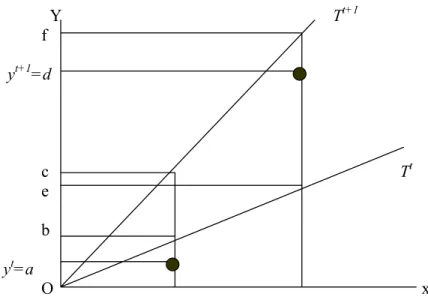
We may illustrate the output-oriented Malmquist productivity index in a figure. In figure 3.2.1, two technologies are involved, one for period t and the other for period t+1.

(30)

19

Figure 3.2.1. Output-Oriented Malmquist Productivity Index

Y Tt+1 f yt+1_=d c Tt e b yt_=a O x

The productivity change for the two input-output vectors (_xt,_yt)_and

) ,

(_xt+1 _yt+1 _{based on y-distances is:}

(3.2.4) 2 1 1 1_, ₎ , , ( _      = + + Of Od Oa Oc Oa Ob Oe Od y x y x M t t t t o

Malmquist productivity index can also be decomposed into efficiency change (MEFFCH) and technical change (MTECH) components. These two components can be defined as:

(3.2.5) ) , ( ) , ( 1 1 1 t t t o t t t o y x D y x D MEFFCH + + + = and (3.2.6) 2 1 1 1 1 1 1 1 ) , ( ) , ( ) , ( ) , (       = ₊ +₊ +₊ _t₊ _t _t o t t t o t t t o t t t o y x D y x D y x D y x D MTECH

The Malmquist productivity index is simply the product of these two components, namely:

(31)

20 (3.2.7) +1 ₌ +1_⋅ t+1. t t t t t MEFFCH MTECH M

In figure 3.2.1, efficiency change and technical change components can be defined as: (3.2.8) Oa Ob Of Od MEFFCH = and (3.2.9) 2 1     = Ob Oc Oe Of MTECH

This index has several desirable features such that as opposed to alternative indices like Fischer and Törnquist, it does not require any price information on outputs and inputs. However, although in principle Malmquist productivity index can be used to measure the productivity in the presence of bads, the underlying distance functions does not allow us to credit our individual observations for reductions in pollutants. If we try to incorporate the bads into productivity by employing Malmquist productivity index, the output distance functions can be represented as:

(3.2.10) D_o(x,y,b)=inf{θ:((y,b/θ))∈P(x)}

However, the output distance function in (3.2.10) without crediting the reduction of bads, expands the desirable and undesirable output set (y, b) proportionally as much as it is feasible. This is the major deficiency of this index when we consider the joint production of goods and bads. Further discussion of this point can be seen in Chung et al. (1997).

(32)

21

3.3. Malmquist-Luenberger Productivity Index

This modified version of original Malmquist productivity index is first developed in Chung et al. (1997) and to represent technology, rather than using Shephard output distance functions, employs directional output distance functions. This approach credits the firms or countries for the reduction of undesirable outputs by seeking to increase the good outputs while simultaneously decreasing the bads. We may formulate the directional distance functions as:

(3.3.1) Do(x,y,b;g)=sup{β :(y,b)+βg∈P(x)} ρ

where g is the vector of directions which is defined as g = (y, -b). It is also possible to construct a relation between Shephard and directional distance functions. By 3.3.1, by letting g = (y, b) we may write:

(3.3.2) 1 ) , , ( 1 } 1 ) , , ( 1 : sup{ } 1 ) , , ( ) 1 ( : sup{ } 1 )) , ( ) , ( , ( : sup{ ) , ; , , ( − = − ≤ = ≤ + = ≤ + = b y x D b y x D b y x D b y b y x D b y b y x D o o o o o β β β β β β ρ and therefore: (3.3.3) Dρ_o(x,y,b;y,b)=(1/D_o(x,y,b))−1 or equivalently (3.3.4) Do(x,y,b)) 1/(1 Do(x,y,b;y,b)) ρ + =

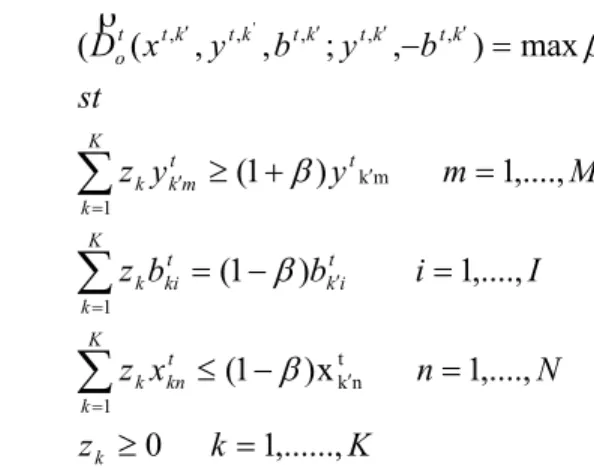
Similar to Shephard distance functions, directional distance functions can also be computed as a solution to linear programming problems. We can formalize such a problem for k`:

(33)

22 (3.3.5) K k z N n x z I i b b z M m y y z st b y b y x D k K k t kn k K k t i k t ki k K k t t m k k k t k t k t k t k t t o ,..., 1 0 ,...., 1 x ) 1 ( ,...., 1 ) 1 ( ,...., 1 ) 1 ( max ) , ; , , ( ( 1 t n k 1 1 m k , , , , , ' = ≥ = − ≤ = − = = + ≥ = −

∑

= ′ = ′ = ′ ′ ′ ′ ′ ′ β β β β ρ

To make a more precise distinction between the directional and Shephard type distance functions, we may refer to figure 3.3.1.

Figure 3.3.1. Distance Functions

y (good)

g

In Figure 3.3.1, the output set is defined by P(x). As already introduced, this output set is defined by goods (y) and bads (b) on the y- and x-axis respectively. We may refer to the Shephard distance functions by the value OC/OA. If the firm

(y, b) P(x) b (Bad) O A C B

(34)

23

or country increases both goods and bads by this value, then it is judged as efficient. In contrast, for directional distance functions, we should refer the ratio BC/Og. That is, the directional distance function starts at C and scales in the direction of increased goods and decreased bads and projects C on the boundary at B. Then the firm or country is called efficient if it moved from C to B. This actually implies a reduction in bads and an increase in goods.

After making this distinction between the directional and Shephard distance functions, we may follow Chung et al. (1997) to write the Malmquist-Luenberger productivity index. By letting g = (y, -b), the output-oriented Malmquist Luenberger productivity index is:

(3.3.6) 2 1 1 1 1 1 1 1 1 1 1 1 1 1 1 )) , ; , , ( 1 ( )) , ; , , ( 1 ( )) , ; , , ( 1 ( )) , , , ( 1 (       − + − + − + − + = ₊ ₊ ₊ ₊ ₊ ₊ +₊ ₊ ₊ ₊ ₊ + t t t t t t o t t t t t t o t t t t t t o t t t t t o t t b y b y x D b y b y x D b y b y x D b b y x D ML ρ ρ ρ ρ

Note that if the direction function g = (y, b), this index coincides with the original Malmquist index. As all Malmquist type indices, this index can also be decomposed into efficiency change and technical change components. The efficiency component is:

(3.3.7) ) , ; , , ( 1 ) , , , ( 1 1 1 1 1 1 1 1 + + + + + + + − + − + = _t _t _t _t _t _t o t t t t t o t t b y b y x D b b y x D MLEFFCH ρ ρ

(35)

24 (3.3.8) 2 1 1 1 1 1 1 1 1 1 1 1 1 1 1 )) , ; , , ( 1 ( )) , ; , , ( 1 ( )) , , , ( 1 ( )) , , , ( 1 (       − + − + − + − + = + + ₊+ ₊+ ₊+ ₊+ ₊+ + t t t t t t o t t t t t t o t t t t t o t t t t t o t t b y b y x D b y b y x D b b y x D b b y x D MLTECH ρ ρ ρ ρ

and as in the Malmquist index the product of these two components gives the Malmquist-Luenberger Index. (3.3.9) +1 ₌ +1_⋅ t+1. t t t t t MLEFFCH MLTECH ML

3.4. Index Number Approach

In this section, an environmental performance index developed in Fare et al. (1999) is adopted. Basically the index they defined is the ratio of two indices namely good output quantity index and bad output quantity index. These indices are developed using a DEA framework and distance functions like Malmquist index. However in contrast to Malmquist index, this index employs sub-vector distance functions since it scales the good and bad outputs separately. It also satisfies the properties of closedness and convexity due to Fare and Primont (1995). We may formally define a sub-vector distance functions for good outputs as:

(3.4.1) D_y(x,y,b)=inf{θ:(x,y/θ,b)∈T}

This distance function holds the inputs and bad outputs fixed and expands the good outputs as much as is feasible. Note that it is also homogeneous of degree +1 in y . Keeping the notation used, let _{x and}0 _{b be our given inputs and bad}0

(36)

25

outputs, then the good output index compares two output vectors _{y and}k _{y by}l

taking the ratio of two distance functions. Then, the good index is: (3.4.2) ) , , ( ) , , ( ) , , , ( ₀ ₀ 0 0 0 0 b y x D b y x D y y b x Q _l y k y l k y = .

On the other hand, the index of bad outputs is constructed using an input distance function approach. The input based distance function for bad outputs can be written as

(3.4.3) D_b(x,y,b)=sup{λ:(x,y,b/λ)∈T}.

This distance function is homogeneous of degree +1 in bad outputs, and it is defined by finding the maximal contraction in these outputs. Given (_x0,_y0)_{, the} quantity index of bad outputs compares _{b and}k _{b and can be defined using the}l

ratios of distance functions such that: (3.4.4) ) , , ( ) , , ( ) , , , ( ₀ ₀ 0 0 0 0 l b k b l k b b y x D b y x D b b y x Q = .

The bad index defined in (3.4.4) with the good index defined in 3.4.2 satisfies some desirable index number properties due to Fischer (1922). These desirable properties for bad index are:

(3.4.5) Homogeneity: ( 0, 0, , ) ( 0, 0, k, l) b l k b x y b b Q x y b b Q λ =λ (3.4.6) Time-reversal: ( 0, 0, , ) ( 0, 0, k, l)₌1 b l k b x y b b Q x y b b Q (3.4.7) Transitivity: ( 0, 0, , ) ( 0, 0, , ) ( 0, 0, k, l) b l k b l k b x y b b Q x y b b Q x y b b Q = (3.4.8) Dimensionality: ( 0, 0, , ) ( 0, 0, k, l) b l k b x y b b Q x y b b Q λ λ =

(37)

26

The environmental performance index of Fare et al. (1999) is the ratio of good and bad indices, i.e.:

(3.4.9) ) , , , ( ) , , , ( ) , , , , , , ( . l k 0 0 b l k 0 0 y l k l k 0 0 0 l k b b y x Q y y b x Q b b y y b y x E =

This performance index allows us to evaluate how much good output is produced per bad output. If we consider a simple case where there is only one good and one bad output is produced, this index can be written in the following form due to homogeneity of the component distance functions.

(3.4.10) l l k k l k b y b y E . =

This one bad one good index states that the index is the ratio of average good per bad output for kand l.

(38)

27

CHAPTER 4 DATA, APPLICATION AND COMPARISON

This chapter first presents the data used in this thesis. Then, the following sub sections summarize the application of the data and comparison of our Malmquist and Malmquist-Luenberger indices. Final section is reserved for the application of environmental efficiency index.

4.1. The Data

Basically, in a production process for a given inputs, good (desirable) and bad (undesirable or hazardous) outputs are produced. Our resource constraint (inputs) in constructing the Malmquist and Malmquist-Luenberger Productivity indices and environmental performance index are represented by net fixed standardized capital stock and labor (number of employed workers). As a good (desirable) output, GDP, purchasing power parity (PPP) adjusted with 1996 prices is used. Our proxies for hazardous outputs are industrial CO2 (carbon dioxide) and NOx

(nitrogen oxide) emissions and organic water pollutant emissions.

The data on capital stock, labor and GDP are compiled from a recent data set (Marquetti, 2002). World Development Indicators (World Bank, 2002) are used for CO2 and organic water emissions whereas NOx emissions are compiled from

(39)

28

Our annual data set includes 28 OECD countries. Slovak Republic and Czech Republic are excluded because of the unavailability of the data for these countries. The time period considered is 16 years, 1983 to1998. In table 4.1.1 we present the data as the average of 16 years for each of the OECD countries.

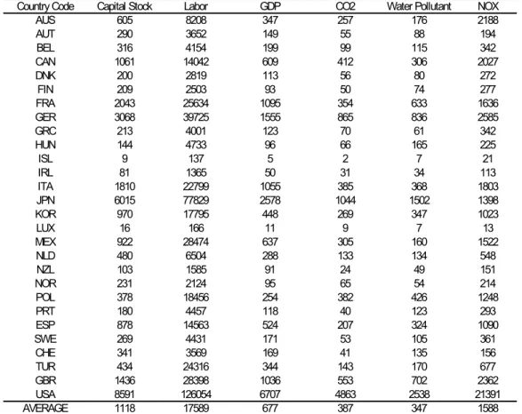
Table 4.1.1. The Data as the Average of the Period 1983-1998

Country Code Capital Stock Labor GDP CO2 Water Pollutant NOX

AUS 605 8208 347 257 176 2188 AUT 290 3652 149 55 88 194 BEL 316 4154 199 99 115 342 CAN 1061 14042 609 412 306 2027 DNK 200 2819 113 56 80 272 FIN 209 2503 93 50 74 277 FRA 2043 25634 1095 354 633 1636 GER 3068 39725 1555 865 836 2585 GRC 213 4001 123 70 61 342 HUN 144 4733 96 66 165 225 ISL 9 137 5 2 7 21 IRL 81 1365 50 31 34 113 ITA 1810 22799 1055 385 368 1803 JPN 6015 77829 2578 1044 1502 1398 KOR 970 17795 448 269 347 1023 LUX 16 166 11 9 7 13 MEX 922 28474 637 305 160 1522 NLD 480 6504 288 133 134 548 NZL 103 1585 91 24 49 151 NOR 231 2124 95 65 54 214 POL 378 18456 254 382 426 1248 PRT 180 4457 118 40 123 293 ESP 878 14563 524 207 324 1090 SWE 269 4431 171 53 105 361 CHE 341 3569 169 41 135 156 TUR 434 24316 344 143 170 677 GBR 1436 28398 1036 553 702 2362 USA 8591 126054 6707 4863 2538 21391 AVERAGE 1118 17589 677 387 347 1588

Capital Sock: Estimated Net Fixed Standardized Capital Stock (billion $) Labor: Number of Workers ( '000 workers)

GDP: Gross Domestic Product (1996, PPP) (billion $) CO2: Carbon Dioxide Emissions, Industrial ( '000 kt)

Water Pollutant: Organic Water Pollutant (BOD) Emissions ( '000 kg per day) NOX: Nitrogen Oxide Emissions ( ' 000 kt)

(40)

29

Note that, carbon dioxide and nitrogen oxide emissions from industrial processes are those stemming from the burning of fossil fuels and the manufacture of cement. They include contributions to the carbon dioxide and nitrogen oxide produced during consumption of solid, liquid, and gas fuels and gas flaring. On the other hand, Emissions of organic water pollutants are measured by biochemical oxygen demand, which refers to the amount of oxygen that bacteria in water will consume in breaking down waste. This is a standard water-treatment test for the presence of organic pollutants.

4.2. Malmquist and Malmquist-Luenberger Indices, Application

We begin our analysis by computing the Malmquist productivity index including only good outputs. In table 4.2.1, we report the Malmquist productivity index and its decomposition into technical and efficiency change for the time period 1985 to 1998 by sequential multiplication of the improvements in each sub-period. Recall that values greater than unity indicate an improvement in productivity performance, while values less than unity implies deterioration. Remarkably, all OECD countries improved their productivity during the time span considered except Canada, Japan, Korea, New Zealand, Portugal, Switzerland, and Great Britain. Clearly, Ireland, Luxembourg and Finland are best performers and generate substantial productivity growth. Moreover, the results suggest that technical change dominates efficiency change as a source of productivity growth. We may also say that OECD countries improved their productivity approximately %3 for the 1985-1998 period. For a detailed exposition, in appendix B, tables 4.2.3, 4.2.4 and 4.2.5 presents the Malmquist productivity

(41)

30

index and its decomposition into technical and efficiency change respectively for all OECD countries and each sub period considered.

Table 4.2.1. Malmquist Productivity Index and Decomposition: 1985-1998

In constructing our Malmquist-Luenberger productivity index, we assume the joint production of goods and bads. This approach credits the countries for reduction of undesirable outputs by seeking to increase the good outputs while simultaneously decreasing the bads. Although our data set includes three undesirable outputs, we do not compute a Malmquist-Luenberger index that simultaneously decreases all three, since such an attempt creates too many

Country Code Malmquist Index Technical Change Efficiency Change Rank

AUS 1,0792 1,1296 0,9555 14 AUT 1,0767 1,1362 0,9477 15 BEL 1,0030 1,0673 0,9398 22 CAN 0,9632 1,0822 0,8901 23 DNK 1,0741 1,1026 0,9745 16 FIN 1,4701 1,3460 1,0925 3 FRA 1,1124 1,1442 0,9722 11 GER 1,1174 1,1466 0,9747 10 GRC 1,2583 0,9900 1,2713 6 HUN 1,0574 1,0158 1,0412 17 ISL 1,1905 1,0990 1,0833 7 IRL 1,6419 0,9890 1,6604 1 ITA 1,1110 1,1563 0,9610 12 JPN 0,9221 1,0061 0,9166 27 KOR 0,7514 0,9955 0,7546 29 LUX 1,4987 1,4987 1,0000 2 MEX 1,1715 1,0128 1,1568 8 NLD 1,1209 1,1584 0,9678 9 NZL 0,9535 0,9882 0,9651 25 NOR 1,2871 1,4898 0,8640 5 POL 1,4619 1,0416 1,4035 4 PRT 0,9366 1,0026 0,9340 26 ESP 1,0099 0,9871 1,0231 21 SWE 1,0797 0,9855 1,0956 13 CHE 0,8850 1,4007 0,6318 28 TUR 1,0133 1,0509 0,9645 20 GBR 0,9558 0,9921 0,9634 24 USA 1,0251 1,0303 0,9948 19 GEOMEAN 1,0288 1,0579 0,9727 18

(42)

31

infeasible solutions. Following Fare et al. (2001), in order to reduce the number of infeasible solutions, we further assumed that each year’s technology is determined by observations on inputs and outputs of current and past two periods. Considering our pollutant data, we computed four different Malmquist-Luenberger productivity indices. These indices credit the reduction of only CO2,

NOX and CO2, NOX and organic water pollutant and NOX and water pollutant

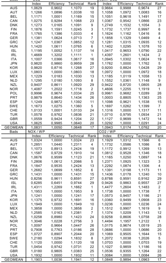
respectively. In table 4.2.2 we report the Malmquist-Lenberger productivity indices and their decompositions into efficiency and technical change for each of the OECD countries for the period 1985-1998. Although rankings of countries differ according to the pollutants included, Ireland and Norway are best performers in all indices. We also observe that technical change dominates efficiency change in all Malmquist-Luenberger productivity indices computed. Moreover, Poland and Luxembourg are the countries that all indices yield infeasible solutions for some years. All our indices indicate an approximately %8 productivity growth for OECD countries on average except the one which credits the reduction in NOX and organic water pollutant. This index indicates a %19

(43)

32

Table 4.2.2. Malmquist-Luenberger Indices and Decompositions: 1985-1998

Bads CO2 NOX / CO2

Index Efficiency Technical Rank Index Efficiency Technical Rank AUS 1,0629 0,9602 1,1070 19 0,9664 0,9988 0,9674 27 AUT 1,1266 1,0896 1,0338 10 1,1058 1,0972 1,0083 16 BEL 1,1171 1,0001 1,1169 15 1,1051 0,9618 1,1491 17 CAN 1,0275 0,9284 1,1068 23 1,0367 0,9542 1,0866 23 DNK 1,1273 1,0165 1,1091 9 1,2749 1,1532 1,1054 3 FIN 1,1876 1,1591 1,0245 3 1,1732 1,1737 0,9997 6 FRA 1,1765 1,1386 1,0333 4 1,1624 1,1162 1,0416 8 GER 1,1381 1,0624 1,0713 7 1,1858 1,1329 1,0469 4 GRC 1,1247 1,0367 1,0852 12 1,1281 1,0315 1,0935 12 HUN 1,1420 1,0611 1,0765 6 1,1402 1,0295 1,1078 10 ISL 1,1195 1,0052 1,1137 14 1,0417 0,9653 1,0790 22 IRL 1,4669 1,3202 1,1111 1 1,4397 1,2601 1,1424 2 ITA 1,1007 1,0366 1,0617 16 1,0945 1,0302 1,0624 19 JPN 0,9820 0,9860 0,9959 28 1,1762 1,0000 1,1762 5 KOR 0,9820 0,8716 1,1268 27 0,9200 0,8824 1,0428 29 LUX 1,0803 1,0000 1,0803 18 1,0972 1,0000 1,0972 18 MEX 1,1229 1,0183 1,1030 13 1,1185 1,0119 1,1058 13 NLD 1,1295 1,0180 1,1093 8 1,1552 1,0361 1,1148 9 NZL 0,9407 0,8611 1,0920 29 0,9422 0,8720 1,0805 28 NOR 1,4087 1,2022 1,1718 2 1,4606 1,2255 1,1919 1 POL 0,9996 0,9674 1,0334 25 0,9961 0,9682 1,0289 26 PRT 0,9879 0,8640 1,1434 26 1,0003 0,8805 1,1363 25 ESP 1,1249 0,9872 1,1392 11 1,1098 0,9621 1,1538 15 SWE 1,1673 1,0275 1,1360 5 1,1697 1,0262 1,1399 7 CHE 1,0133 1,0001 1,0133 24 1,1316 1,0000 1,1317 11 TUR 1,0578 0,9762 1,0836 21 1,0710 0,9795 1,0934 21 GBR 1,0559 0,9424 1,1204 22 1,1127 0,9699 1,1472 14 USA 1,0625 0,9985 1,0640 20 1,0292 1,0000 1,0291 24 GEOMEAN 1,0831 1,0050 1,0648 17 1,0943 1,0174 1,0762 20

Bads NOX / W P CO2 / W P

Index Efficiency Technical Rank Index Efficiency Technical Rank AUS 1,0324 1,0000 1,0324 23 1,1929 1,0312 1,1566 6 AUT 1,2851 1,0440 1,2311 4 1,1732 1,0586 1,1086 8 BEL 1,1073 0,8913 1,2424 19 1,1172 0,9912 1,1269 13 CAN 1,1587 0,9729 1,1910 14 1,0812 0,9528 1,1346 18 DNK 1,0676 0,9599 1,1123 21 1,1165 1,0250 1,0897 14 FIN 1,2806 1,0612 1,2066 5 1,2371 1,0925 1,1323 3 FRA 1,1847 0,9535 1,2424 13 1,2292 1,0874 1,1306 4 GER 1,2682 1,0699 1,1852 6 1,1391 1,0198 1,1173 11 GRC 1,1431 1,0000 1,1431 15 1,1436 1,0178 1,1240 10 HUN 0,8256 0,9611 0,8591 27 0,8788 0,9591 0,9162 29 ISL 0,6285 0,6451 0,9744 29 0,9426 0,9863 0,9557 27 IRL 1,4311 1,2269 1,1662 1 1,4477 1,2604 1,1483 2 ITA 1,1953 1,0000 1,1953 9 1,1738 1,0000 1,1738 7 JPN 1,1241 1,0000 1,1241 17 1,0573 0,9457 1,1186 21 KOR 1,1375 0,9732 1,1691 16 1,0360 0,9499 1,0908 23 LUX 1,1949 1,0000 1,1949 10 1,0236 1,0000 1,0236 24 MEX 1,3858 1,0000 1,3858 2 1,1512 0,9907 1,1619 9 NLD 1,2585 1,0163 1,2381 7 1,1374 1,0209 1,1143 12 NZL 1,0258 0,8980 1,1423 24 0,9258 0,8606 1,0758 28 NOR 1,3046 1,0228 1,2756 3 1,4494 1,1957 1,2122 1 POL 1,0097 0,9664 1,0447 26 1,0175 0,9674 1,0519 25 PRT 0,7908 0,7763 1,0186 28 1,0686 1,0000 1,0686 20 ESP 1,0727 0,8907 1,2044 20 1,1069 0,9505 1,1644 15 SWE 1,2180 1,0294 1,1832 8 1,2072 1,0038 1,2026 5 CHE 1,1120 1,0000 1,1120 18 1,0703 1,0000 1,0703 19 TUR 1,0454 0,9742 1,0731 22 1,1027 0,9859 1,1186 16 GBR 1,0180 0,9805 1,0383 25 1,0536 0,9355 1,1264 22 USA 1,1932 1,0000 1,1932 11 1,0084 1,0000 1,0084 26 GEOMEAN 1,1903 1,0036 1,1941 12 1,0848 0,9894 1,0963 17

(44)

33

For a detailed presentation, we report each of the Malmquist-Luenberger indices and their decompositions into technical and efficiency change for all countries and sub periods in appendix B, in tables 4.2.6 to 4.2.17. In each of the tables we also report the years in which infeasible solution for the individual countries occur.

4.3. Malmquist and Malmquist-Luenberger Indices, Comparison

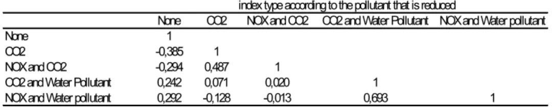
Clearly, our Malmquist-Luenberger indices suggest a higher productivity growth for OECD countries. This result is expected since Malmquist productivity index does not account for the joint production of goods and bads while Malmquist-Luenberger index does. On the other hand, our Malmquist-Malmquist-Luenberger indices considerably differ according to the spearman correlations. This finding is consistent with our assumptions since we employ different pair of pollutants in the computation of these indices. The spearman correlations between Malmquist productivity index and Malmquist-Luenberger productivity indices are presented in table 4.3.1 below.

Table 4.3.1. Spearman Correlations of Indices

Note that rather than individual sub-periods, these correlations are computed for the whole period 1985-1998. The highest correlation between the Malmquist

None CO2 NOX and CO2 CO2 and Water Pollutant NOX and Water pollutant

None 1

CO2 -0,385 1

NOX and CO2 -0,294 0,487 1

CO2 and Water Pollutant 0,242 0,071 0,020 1

NOX and Water pollutant 0,292 -0,128 -0,013 0,693 1

(45)

34

index and Malmquist-Luenberger index is –0.385. Negative correlation between indices indicates that Malmquist and Malmquist-Luenberger indices move in opposite directions during a negative or positive movement in pollutants.

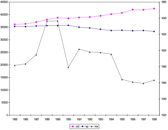
If we consider the annual sub-periods where our pollutants have an increasing path, we would expect that a measure of productivity that explicitly accounts for the joint of goods and bads (Malmquist-Luenberger indices) would exhibit a slower growth than the conventional measures that ignore bads (Malmquist index). However this expectation may not hold if our pollutants move in opposite directions during the time period considered or if there exist a dramatic increase or decrease in the trend of any pollutant. To observe these facts, we first present the trend of pollution emissions of OECD countries in figure 4.3.1.

Figure 4.3.1. The Trend of Pollution Emissions in OECD

0 50000 100000 150000 200000 250000 300000 350000 400000 450000 1985 1986 1987 1988 1989 1990 1991 1992 1993 1994 1995 1996 1997 1998 1520 1540 1560 1580 1600 1620 1640 1660 co2 wp nox

(46)

35

The pollutant data for each year is simply calculated by taking the average of 28 individual OECD countries for the period considered. We can clearly see that CO2 has an increasing path for all years. For NOX and organic water pollutant

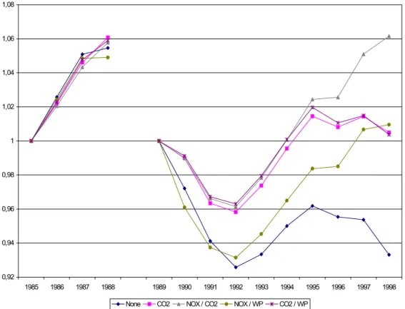
data, 1989 can be considered as a break point. Both pollutants increase until 1989 and then decrease for the following years. For the next step, we present the trends in our Malmquist and Malmquist-Luenberger indices together in figure 4.3.2 and try to observe their respective movements according to the changes in undesirable outputs.

Figure 4.3.2. The Trend of Indices for OECD

For the sub period 1985-1989, the figures 4.3.1 and 4.3.2 support our expectation. During this period, all pollutants have an upward trend. So, we

0,95 0,97 0,99 1,01 1,03 1,05 1,07 1,09 1,11 1,13 1985 1986 1987 1988 1989 1990 1991 1992 1993 1994 1995 1996 1997 1998 None CO2 NOX / CO2 NOX / WP CO2 / WP

(47)

36

would expect our Malmquist index to over estimate the productivity growth compared to Malmquist-Luenberger indices. For the period 1990-1998, we have an upward trend in CO2. So, for this sub period, we again expect our Malmquist

index to dominate the Malmmquist-Luenberger index that credits the reduction in CO2. However figure 4.3.2 indicates that Malmquist-Luenberger index exhibits

higher productivity growth than the Malmquist index for the time period considered. This fact may be justified if we consider the individual countries rather than the whole sample. We also observe that until 1989 almost all countries have an increasing figure of CO2. However during the period

1990-1998, some countries that has a large weight of CO2 in the whole sample has a

downward trend. Such an example (Great Britain) will be presented later. For the other pollutants considered, the results support our expectations. Obviously, Malmquist index has a slower growth than the Malmquist-Luenberger index that credits the reduction of NOX and organic water pollutant during the period

1990-1998 in which both pollutants considered have a downward trend. For the Malmquist-Luenberger indices that credits reduction in NOX and CO2 and CO2

and organic water pollutant, the results may be misleading since CO2 increases

while the other two undesirable outputs decrease during the time span considered. However by taking figure 4.3.2 as our reference, we may say that reductions in NOX and organic water pollutants dominate the increases in CO2.

If we turn our attention to individual countries, we again see that our expectations are consistent with the findings. We first choose Great Britain since for all indices; it does not give any infeasible solutions for the whole sub-periods. We again start with the presentation of the annual trends of the pollution emissions for Great Britain in figure 4.3.3.

(48)

37

Figure 4.3.3. The Trend of Pollution Emissions in Great Britain

We can clearly observe that in Great Britain, NOX increases until 1989 while

organic water pollutant and CO2 has a smooth trend for the same period. Also,

NOX and organic water pollutant have a downward trend in the period 1989-1998

while CO2 again seems constant for the same period. To make a comparison, we

illustrated the Malmquist and Malmquist-Luenberger productivity indices for Great Britain in figure 4.3.4.

0,00E+00 1,00E+05 2,00E+05 3,00E+05 4,00E+05 5,00E+05 6,00E+05 7,00E+05 8,00E+05 1985 1986 1987 1988 1989 1990 1991 1992 1993 1994 1995 1996 1997 1998 0 500 1000 1500 2000 2500 3000 co2 wp nox

(49)

38

Figure 4.3.4. The Trend of Indices for Great Britain

Until 1989 we can clearly see that Malmquist index shows a higher productivity growth than all Malmquist-Luenberger indices. This finding is consistent with our expectations since for that period NOX has a very significant upward trend.

We also observe that for the period 1987-1988, Malmquist-Luenberger index that credits the reduction in CO2 produces higher productivity growth rates than the

Malmquist index, because of the reduction in the CO2 for the same period. For

the other sub periods 1989-1998, we observe that our Malmquist-Luenberger indices exhibit higher productivity growth than the Malmquist index. This is again expected since for the same time period, the pollutant data for Great Britain has a downward trend.

0,92 0,94 0,96 0,98 1 1,02 1,04 1,06 1,08 1985 1986 1987 1988 1989 1990 1991 1992 1993 1994 1995 1996 1997 1998 None CO2 NOX / CO2 NOX / WP CO2 / WP

(50)

39

Our second sample country is Norway as one of the best performers in all indices. The path of pollutants in Norway during the time period 1985-1998 is presented in figure 4.3.5.

Figure 4.3.5. The Trend of Pollution Emissions in Norway

A quick glance at figure 4.3.5 reveals that organic water pollutant data for Norway has a downward trend for the whole period. NOX is decreasing until

1992 and has an upward trend for the other sub-periods. CO2 data for Norway

has a fluctuating trend. It decreases until 1989, then increases from 1989-1996 and for the last two years it decreases again. To make clear exposition, we

0 20000 40000 60000 80000 100000 120000 1985 1986 1987 1988 1989 1990 1991 1992 1993 1994 1995 1996 1997 1998 195 200 205 210 215 220 225 230 co2 wp nox

(51)

40

present the path of indices for Norway in figure 4.3.6 in four different sub-periods.

Figure 4.3.6. The Trend of Indices for Norway

For the sub-period 1985-1987, we see that our Malmquist index exhibits a higher productivity growth than Malmquist-Luenberger indices since for the same period the pollutant data for Norway has an upward trend. One significant fact is we can clearly observe the dramatic slowdown in CO2 from 1987 to 1988, since

for that period Malmquist-Luenberger index that credits reduction in CO2 clearly

indicates a higher productivity growth than Malmquist index. For the sub period 1989-1991, we expect Malmquist index to produce higher productivity growth

0,95 1 1,05 1,1 1,15 1,2 1985 1986 1987 1988 1989 1990 1991 1992 1993 1994 1995 1996 1997 1998 None CO2 NOX / CO2 NOX / WP CO2 / WP