Image-Space Decomposition Algorithms for
Sort-First Parallel Volume Rendering of
Unstructured Grids*
H ¨USEYIN KUTLUCA [email protected]
Computer Engineering Department, Bilkent University, TR-06533 Ankara, Turkey
TAHSIN M. KUR¸C [email protected]
Computer Science Department, University of Maryland, College Park, MD 20742
CEVDET AYKANAT [email protected]
Computer Engineering Department, Bilkent University, TR-06533 Ankara, Turkey (Received February 26, 1998; final version accepted November 17, 1998)
Abstract. Twelve adaptive image-space decomposition algorithms are presented for sort-first parallel direct volume rendering (DVR) of unstructured grids on distributed-memory architectures. The algo-rithms are presented under a novel taxonomy based on the dimension of the screen decomposition, the dimension of the workload arrays used in the decomposition, and the scheme used for workload-array creation and querying the workload of a region. For the 2D decomposition schemes using 2D workload arrays, a novel scheme is proposed to query the exact number of screen-space bounding boxes of the primitives in a screen region in constant time. A probe-based chains-on-chains partitioning algorithm is exploited for load balancing in optimal 1D decomposition and iterative 2D rectilinear decomposition (RD). A new probe-based optimal 2D jagged decomposition (OJD) is proposed which is much faster than the dynamic-programming based OJD scheme proposed in the literature. The summed-area table is successfully exploited to query the workload of a rectangular region in constant time in both OJD and RD schemes for the subdivision of general 2D workload arrays. Two orthogonal recursive bisection (ORB) variants are adapted to relax the straight-line division restriction in conventional ORB through using the medians-of-medians approach on regular mesh and quadtree superimposed on the screen. Two approaches based on the Hilbert space-filling curve and graph-partitioning are also proposed. An effi-cient primitive classification scheme is proposed for redistribution in 1D, and 2D rectilinear and jagged decompositions. The performance comparison of the decomposition algorithms is modeled by estab-lishing appropriate quality measures for load-balancing, amount of primitive replication and parallel execution time. The experimental results on a Parsytec CC system using a set of benchmark volumet-ric datasets verify the validity of the proposed performance models. The performance evaluation of the decomposition algorithms is also carried out through the sort-first parallelization of an efficient DVR algorithm.
Keywords: direct volume rendering, unstructured grids, sort-first parallelism, image-space decomposi-tion, chains-on-chains partitioning, jagged decomposidecomposi-tion, rectilinear decomposidecomposi-tion, orthogonal recur-sive bisection, Hilbert space-filling curve, graph partitioning
*This work is partially supported by the Commission of the European Communities, Directorate General for Industry under contract ITDC 204-82166, and Turkish Science and Research Council under grant EEEAG-160
1. Introduction
In many fields of science and engineering, computer simulations provide a cheap and controlled way of investigating physical phenomena. The output of these simu-lations is usually a large amount of numerical values, which makes it very difficult for scientists to extract useful information from the data to derive useful conclusions. Therefore, visualizing large quantities of numerical data as an image provides an indispensable tool for researchers. In many engineering simulations, datasets con-sist of numerical values which are obtained at points (sample points) distributed in a volume that represents the physical environment. The sample points consti-tute a volumetric grid superimposed on the volume, and they are connected to some other nearby sample points to form volume elements (cells). Volumetric grids can be divided into two categories as: structured and unstructured. Structured grids are topologically equivalent to the integer lattices, and as such, can easily be repre-sented by a 3D array. In unstructured grids, the sample points in the volume data are distributed irregularly over 3 dimensional (3D) space and there may be voids in the volumetric grid. Unstructured grids are also called cell oriented grids, be-cause they are represented as a list of cells with pointers to the sample points that form the respective cells. With recent advances in generating higher quality adap-tive meshes, unstructured grids are becoming increasingly popular in the simulation of scientific and engineering problems with complex geometries.
There are two major categories of volume rendering methods: indirect and direct. Indirect methods extract intermediate geometrical representation of the data (i.e. isosurfaces), and render those surfaces via conventional surface rendering methods. Direct methods render the data without generating an intermediate representation, hence they are more general, flexible and have the potential to provide more com-plete information about the data being visualized. However, direct methods are slow due to massive computations. Large scale scientific and engineering simulations are usually performed in parallel on distributed-memory architectures. Parallel visual-ization of the vast amount of volumetric data produced by these simulations on the same parallel machine saves the time to transfer the data from the parallel ma-chine to a sequential graphics workstation over possibly slow communication links. Hence, direct volume rendering (DVR) is a good candidate for parallelization on distributed-memory multicomputers.
1.1. Direct volume rendering (DVR)
In general, the DVR methods consist of two main phases. These are resampling and
composition phases, which are in general manipulated in a highly interleaved
man-ner. In the resampling phase, new samples are interpolated by using the original sample points. The rendering method should somehow locate the new sample point in the cell domain, because the vertices of that cell, in which the new sample is be-ing generated, will be used in the interpolation for the new sample. This problem is known as the point location problem. In the composition phase, the new sam-ples generated are mapped to color and opacity values, which are composited to
determine the contribution of the data on a pixel. The composition operation is as-sociative, but not commutative; therefore these color and opacity values should be composited in visibility order. The determination of the correct composition order is known as the view sort problem.
The DVR algorithms for unstructured grids can be classified into three categories:
ray-casting, projection and hybrid [31]. In the ray-casting methods, the image space
is traversed to cast a ray for each pixel, and each ray is followed, sampled and composited along the volume. In the projection methods, the volume is traversed to perform a view-dependent depth sort on the cells. Then, all cells are projected onto the screen, in this sorted order, to find their contributions to the image and composite them. In the hybrid methods, the volume is traversed in object order such that the contributions of the cells to the image are accumulated in image order.
A DVR application contains two interacting domains: object space and image space. The object space is a 3D domain containing the volume data to be visual-ized. The image space (screen) is a 2D domain containing pixels from which rays are shot into the 3D object domain to determine the color values of the respective pixels. Based on these domains, there are basically two approaches for data parallel DVR: object-space parallelism and image-space parallelism. The cells or cell clus-ters constitute the atomic tasks in the object-space parallelism, whereas the pixels or pixel blocks constitute the atomic tasks in the image-space parallelism. The par-allel DVR algorithms can also be categorized according to the taxonomy proposed by Molnar et. al. [18] for parallel polygon rendering. In polygon rendering, the ren-dering process is a pipeline of operations applied to the primitives in the scene. This rendering pipeline has two major steps called geometry processing and rasterization. Molnar et al. [18] provides a classification of parallelism, based on the point of data redistribution step in the rendering pipeline, as sort-first (before geometry pro-cessing), sort-middle (between geometry processing and rasterization), and sort-last (after rasterization). In this taxonomy, the image-space and object-space parallelism in DVR can be considered as the sort-first and sort-last parallelism, respectively.
In sort-last (object-space) parallel DVR, the 3D object domain is decomposed into disjoint subvolumes and each subvolume is concurrently rendered by a distinct processor. At the end of this local rendering phase, incomplete full-screen images are created at each processor. In the pixel-merging phase, these local partial images are merged for composition over the interconnection network. The sort-last paral-lelism is a promising approach offering excellent scalability in terms of the number of primitives it can handle. However, it suffers from high interprocessor communi-cation volume during the pixel merging phase especially at high screen resolutions.
1.2. Sort-first parallel DVR
In sort-first (image-space) parallel DVR, which is the focus of this work, each pro-cessor is initially assigned a subset of primitives in the scene. The screen is decom-posed into regions and each region is assigned to a distinct processor for rendering. The primitives are then redistributed among the processors so that each processor has all the primitives whose projection areas intersect the region assigned to it. The
primitives whose projection areas intersect more than one region are replicated in the processors assigned to those regions. After primitive redistribution, each pro-cessor performs local rendering operations on its region. The sort-first parallelism is a promising approach since each processor generates a complete image for its lo-cal screen subregion. However, it faces load-balancing problems in the DVR of un-structured grids due to uneven on-screen primitive distribution. Hence, image-space decomposition is a crucial factor in the performance of the sort-first parallelism.
The image-space decomposition schemes for sort-first parallel DVR can be clas-sified as static, dynamic and adaptive. Static decomposition is a view-independent scheme and the load-balancing problem is solved implicitly by the scattered assign-ment of the pixels or pixel blocks. The load-balancing performance of this scheme depends on the assumption that neighbor pixels are likely to have equal workload since they are likely to have similar views of the volume. The scattered assignment scheme has the advantage that assignment of screen regions to processors is known a priori and static irrespective of the data. However, since the scattered assignment scheme assigns adjacent pixels or pixel blocks to different processors, it disturbs the image-space coherency and increases the amount of primitive replication. Here, the image-space coherency relies on the observation that rays shot from nearby pixels are likely to pass through the same cells involving similar computations. In addi-tion, since decomposition is done irrespective of input data, it is still possible that some regions of the screen are heavily loaded and some processors may perform substantially more work than the others. In the dynamic approach, pixel blocks are assigned to processors in a demand-driven basis when they become idle. The dynamic approach also suffers from disturbing the image-space coherency since ad-jacent pixel blocks may be processed by different processors. Furthermore, since region assignments are not known a priori, each assignment should be broadcast to all processors so that necessary primitive data is transmitted to the respective pro-cessor. Hence, the dynamic scheme is not a viable approach for message-passing dis-tributed memory architectures. Adaptive decomposition is a view-dependent scheme and the load-balancing problem is solved explicitly by using the primitive distribu-tion on the screen. The adaptive scheme is a promising approach since it handles the load-balancing problem explicitly and it preserves the image-space coherency as much as possible by assigning contiguous pixels to the processors.
1.3. Previous work
Most of the previous work on parallel DVR of unstructured grids evolved on shared-memory multicomputers [3, 5, 29]. Challinger [3, 5] presents image-space paral-lelization of a hybrid DVR algorithm [4] for BBN TC2000 shared-memory multi-computer. In the former work [3], the scanlines are considered as the atomic tasks and they are assigned to the processors using the static (scattered) and dynamic (demand-driven) schemes for two different algorithms. In the latter work [5], the screen is divided into square pixel blocks which are considered as the atomic tasks for dynamic assignment. The pixel blocks are sorted in decreasing order according to the number of primitives associated with them, and they are considered in this
sorted order for dynamic assignment to achieve better load-balancing. Williams [29] presents object-space parallelization of a projection based DVR algorithm [30] on Silicon Graphics Power Series. The target machine is a shared-memory multicom-puter with commulticom-puter graphics enhancement. Ma [15] investigates sort-last paral-lelization of a ray-casting based DVR algorithm [8] on an Intel Paragon multicom-puter which is a message-passing distributed-memory architecture.
1.4. Contributions
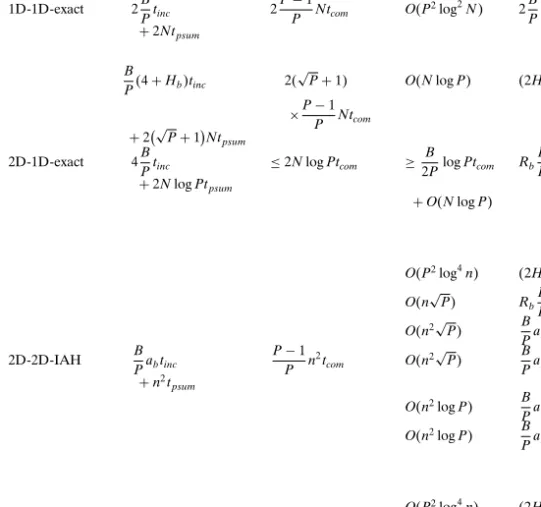
In this work, we investigate sort-first parallelism for DVR of unstructured grids on distributed-memory architectures. This type of parallelism was not previously utilized in DVR of unstructured grids on distributed-memory multicomputers. We present twelve adaptive image-space decomposition algorithms under a novel tax-onomy. The proposed taxonomy is based on the dimension of the screen decom-position and the dimension of the workload arrays used in the decomdecom-position. The decomposition algorithms are parallelized as much as possible to reduce the prepro-cessing overhead. Table 1 displays the acronyms used for the image-space decom-position algorithms listed according to the classification of the proposed taxonomy. As in the previous works on parallel polygon rendering [7, 20, 25, 28], the num-ber of primitives that fall onto a region is used to represent the workload of the region. The screen-space bounding-box of the projection area of a primitive is used to approximate the coverage of the primitive on the screen. The bounding-box ap-proximation is selected to avoid expensive computations needed in finding the
ex-Table 1. The image-space decomposition algorithms
Classification Abbreviation Complete name Primitive classification HHD Heuristic Horizontal Decomposition Inverse-mapping 1D-1D-exact OHD Optimal Horizontal Decomposition Inverse mapping HJD Heuristic Jagged Decomposition Inverse mapping 2D-1D-exact ORB-1D Orthogonal Recursive Bisection with 1D
arrays Rectangle-intersection
OJD-I Optimal Jagged Decomposition using
In-verse area heuristic for workload array Inverse mapping ORB-I Orthogonal Recursive Bisection using
In-verse area heuristic for workload array Rectangle-intersection ORBMM-Q Orthogonal Recursive Bisection with
Me-dians of MeMe-dians on Quadtree Mesh 2D-2D-IAH ORBMM-M Orthogonal Recursive Bisection with
Me-dians of MeMe-dians on cartesian Mesh Mesh HCD Hilbert Curve based Decomposition Mesh GPD Graph Partitioning based Decomposition Mesh OJD-E Optimal Jagged Decomposition using
Ex-act model for workload array Inverse mapping 2D-2D-exact RD Rectilinear Decomposition Inverse mapping
act primitive coverage. All the decomposition algorithms query the bounding-box
counts (bb-counts) of the screen subregions repeatedly during the subdivision
pro-cess. Here, the bb-count of a region refers to the number of bounding boxes inter-secting the region. We show that the exact bb-count of a stripe along one of the dimensions can be found in constant time using two 1D workload arrays. This idea is also exploited in some of the 2D decomposition algorithms producing rectangular subregions in a hierarchical manner through using 1D workload arrays. In a pre-vious work by Muller [20], a heuristic scheme, referred to here as the inverse area
heuristic (IAH), is used to estimate the bb-count of a region using one 2D array.
In this work, we propose a novel scheme, referred to here as the exact model, to query the exact bb-count of a rectangular region in constant time by using four 2D workload arrays. Both IAH and exact models are used in the 2D decomposition algorithms utilizing 2D workload arrays.
We present subdivision algorithms that find optimal decompositions for load-balancing. The load-balancing problem in 1D decomposition is modeled as the well-known chains-on-chains partitioning (CCP) problem [2]. The objective in the CCP problem is to divide a given chain of modules into a number of consecutive subchains such that the load of the most heavily loaded subchain is minimized. An efficient probe-based CCP algorithm is utilized for optimal 1D (horizontal) decom-position. The probe-based CCP algorithm is also exploited for two different 2D decomposition schemes: optimal jagged decomposition (OJD) and heuristic recti-linear decomposition (RD). The proposed OJD scheme is a novel scheme appli-cable to the subdivision of general 2D workload arrays, and it is much faster than the dynamic-programming based OJD scheme proposed in the literature [17]. The summed-area table [6] is successfully exploited to query the workload of a rectan-gular region in constant time in both OJD and RD schemes for the subdivision of general 2D workload arrays.
Three distinct 2D decomposition approaches, which generate non-rectangular regions, are also investigated for image-space decomposition. Two orthogonal re-cursive bisection (ORB) variants are implemented to alleviate the load-imbalance problem due to the straight-line division restriction in the ORB scheme adopted by Mueller [20] (referred to as MAHD in his work). These ORB variants apply the medians-of-medians [23, 27] approach on regular mesh and quadtree superim-posed on the screen. The Hilbert space-filling curve [19, 23, 27] is exploited for image-space decomposition. Finally, image-space decomposition is modeled as a graph-partitioning problem and state-of-the-art graph partitioning tool MeTiS [10] is used for partitioning the generated graph.
Three classification schemes are investigated for primitive redistribution to be performed according to the region-to-processor assignment. A straightforward mesh-based local primitive classification algorithm can be used for the decom-position algorithms that generate both rectangular and non-rectangular regions. However, it is computationally very expensive since it involves tallying the bounding boxes of the primitives. The rectangle-intersection based classification algorithm is more efficient for the decomposition schemes that generate rectangular regions. Furthermore, a much more efficient inverse-mapping based classification scheme is proposed for the 1D horizontal, 2D jagged and 2D rectilinear decomposition
schemes. The proposed scheme exploits the regular structure of the decomposi-tions produced by these schemes so that its complexity per primitive is independent of both the number of processors and the screen resolution.
The load-balancing, primitive-replication and parallel run-time performances of the decomposition algorithms are compared both theoretically and exper-imentally. The theoretical models for the comparison of load-balancing and primitive-replication performances are based on establishing appropriate quality measures. The experimental results on a Parsytec CC system using a set of bench-mark volumetric datasets verify the validity of the proposed quality measures. The performance evaluation of the presented image-space decomposition algorithms is also carried out through sort-first parallelization of Challinger’s [4] hybrid DVR algorithm on a Parsytec CC system.
The rest of the paper is organized as follows. Section 2 presents Challinger’s DVR algorithm [4] and describes its sort-first parallelization. Section 3 summarizes the basic steps involved in the parallel image-space decomposition. The taxonomy of the image-space decomposition algorithms is introduced in Section 4. Section 5 presents the workload-array creation algorithms which enable the efficient query of the workloads associated with the regions during the subdivision phase. The image-space decomposition algorithms are presented and discussed in Section 6. The prim-itive classification algorithms for the redistribution phase are given in Section 7. The models for the theoretical performance comparison of the decomposition algorithms are presented in Section 8. Finally, Section 9 presents the experimental results. 2. DVR algorithm
The sequential rendering algorithm chosen for sort-first parallelization is based on the algorithm developed by Challinger [4]. This algorithm adopts the basic ideas in the scanline Z-buffer based polygon rendering algorithms to resolve the point loca-tion and view sort problems. As a result, the algorithm requires that the volumetric dataset is composed of cells with planar faces. This algorithm does not require con-nectivity information between cells, and it has the power to handle non-convex and cyclic grids. In this work, the volumetric dataset is assumed to be composed of tetra-hedral cells. If a dataset contains volume elements that are not tetratetra-hedral, these elements can be converted into tetrahedral cells by subdividing them [8, 26]. A tetrahedral cell has four points and each face of a tetrahedral cell is a triangle, thus easily meeting the requirement of cells with planar faces. Since the algorithm oper-ates on polygons, the tetrahedral dataset is further converted into a set of distinct triangles. Only triangle information is stored in the data files.
The algorithm starts with an initialization phase which involves the sorting of the triangular faces (primitives) into a y-bucket structure according to their minimum y-values in the screen coordinates. Each entry of the y-bucket corresponds to a scanline on the screen. The algorithm performs the following initialization opera-tions for each successive scanline on the screen. Active primitive and active edge lists for the current scanline are updated incrementally. The active primitive list stores the triangles intersecting the current scanline, and it is updated incrementally using
the y-bucket. The active edge list stores the triangle edges intersecting the current scanline. Finally, a span is generated for the active edge pair of each triangle in the active primitive list, and it is sorted into an x-bucket according to its minimum x value. Each entry of the x-bucket corresponds to a pixel location on the current scanline.
Each successive pixel on a scanline is processed as follows. An active span-list is maintained and updated incrementally along the scanline. Each entry of the active span-list stores the z coordinate of the intersection point (z-intersection) of the primitive that generates the span with the ray shot from the respective pixel location, span information, a pointer to the primitive, and a flag to indicate whether the primitive is an exterior or an interior face of the volume. If a face of a cell is shared by two cells, that face is called interior. If it is not shared by any other cell, the face is called exterior. The spans in the active span-list are maintained in sorted increasing order according to their z-intersection values. The z-intersection values are calculated by the incremental rasterization of the spans stored in the x-bucket. Two consecutive spans in the list, if at least one of them belongs to an interior triangle, correspond to the entry and exit faces of a tetrahedral cell hit by the respective ray in the visibility order. As the entry and exit point z values are known from the z-intersection values, a new sample is generated in the middle of the line segment, which is formed by the entry and exit points of the respective ray intersecting the cell, through 3D inverse-distance interpolation of the scalar values at the corner points of the respective triangles. The color and opacity values computed through mid-point sampling along the ray within the cell are composited to the pixel.
The algorithm exploits image-space coherency for efficiency. The calculations of intersections of triangular faces with the scanline, and insertion and deletion oper-ations on the active primitive list are done incrementally. This type of coherency is called inter-scanline coherency. The z-intersection calculations through span ras-terization, depth-sorting of active spans according to their z-intersection values, insertion to and deletion from the active span-list are done incrementally. This type of coherency is called intra-scanline coherency.
2.1. Workload model
As mentioned earlier, the number of primitives that falls onto a region is used to approximate the workload of the region through bounding-box approximation. This workload model is used in the presented image-space decomposition algorithms for the sake of general performance evaluation of sort-first parallel DVR. However, there are three parameters affecting the computational load of a screen region in Challinger’s DVR algorithm [4]. The first one is the number of triangles (primi-tives), because the total workload of a region due to the transformation of triangles, insertion operations into the y-bucket, and insertions into and deletions from the active primitive list is proportional to the number of triangles in the region. The second parameter is the number of scanlines each triangle extends. This parame-ter represents the computational workload associated with the construction of the
edge intersections (hence, corresponding spans), edge rasterization, clipping spans to the region boundaries, and insertion of the spans into the x-bucket. The total number of pixels generated through the rasterization of these spans is the third pa-rameter affecting the computational load of a region. Each pixel generated adds computations required for sorting, insertions to and deletions from the active-span list, and interpolation and composition operations. Therefore, the workload (WL) in a region can be approximated as;
WL = αTNT + αSNS+ αPNP: [1]
Here, NT, NS, and NP represent the number of triangles, spans, and pixels,
respec-tively, to be processed in a region. In Eq. 1, αT, αS; and αP represent the relative
unit computational costs of the operations associated with triangles, spans, and pix-els, respectively.
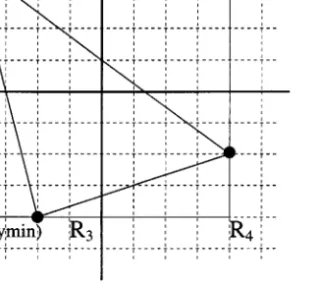
Finding the exact number of spans and pixels generated in a region due to a triangle requires the rasterization of the triangle. The bounding-box approximation used in finding the bb-count of a region is also exploited for estimating the span and pixel counts of the region. That is, a triangle whose bounding box has corner points (xmin; ymin) and (xmax; ymax) is assumed to generate ymax− ymin+ 1 spans and ymax− ymin+ 1 × xmax− xmin+ 1 pixels. It is clear that the bounding-box approximation incurs errors in the estimation of the pixel count of a region in both 1D and 2D decompositions. The bounding-box approximation may also incur errors in the estimation of the span count of a region in 2D decompositions. For example, the triangle shown in Figure 1 contributes only one span to the span count of region R2, while contributing four spans to the span counts of the other three regions R1, R3 and R4. However, the bounding-box approximation incurs four spans for each
one of the four regions, thus inducing error in the estimation of the span count of region R2.
It should be noted here that only the bb-counts are considered in the workload model in the discussion of the image-space decomposition algorithms for the sake of clarity of the presentation. The pixel and span counts can easily be incorporated into the workload model by treating each span and pixel covered by the bounding box of the triangle as bounding boxes of proper height and width with computational loads of αSand αP, respectively. As will be discussed in Section 9, incorporating the span and pixel counts into the workload model substantially increases the performance of the parallelization of Challinger’s DVR algorithm [4] through better load balancing. 3. Parallel image-space decomposition
Parallel adaptive image-space decomposition on distributed-memory architectures involves five consecutive phases: bounding-box creation, local workload-array cation, global-sum operation on local workload arrays, subdivision and primitive re-distribution. In the bounding-box creation phase, processors concurrently create the screen-space bounding boxes of their local primitives. In the workload-array creation phase, processors concurrently create their local workload arrays using the
Figure 1. The bounding-box approximation.
distribution of their local bounding boxes on the full screen. Then, a global-sum operation is performed on the local arrays so that all processors receive the copies of the global workload array(s). In the subdivision phase, the screen is subdivided into P regions using the workload arrays so that each processor is assigned to a single region. In some of the decomposition schemes, the subdivision operation is also performed in parallel, whereas in the other schemes the subdivision operation is not parallelized because of either the sequential nature or the fine granularity of the subdivision algorithm. The schemes adopting parallel subdivision necessitate a final all-to-all broadcast operation so that each processor gets all the region-to-processor assignments. In the redistribution phase, region-to-processors concurrently classify their local primitives according to the region-to-processor assignments. Then, the primitives concurrently migrate to their new home processors through an all-to-all personalized communication operation.
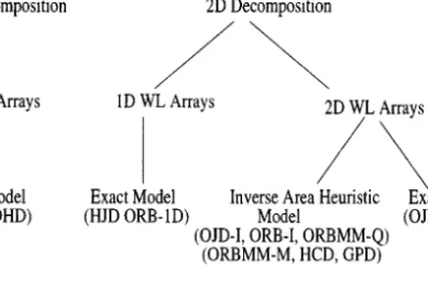
4. A taxonomy of the decomposition algorithms
The taxonomy (see Figure 2) proposed for the image-space decomposition algo-rithms is based on the decomposition strategy and workload arrays used in the decomposition. The first classification is based on the dimension of the decomposi-tion of the screen, which is a 2D space. The 1D decomposidecomposi-tion algorithms divide in only one dimension of the screen. These algorithms utilize the workload distribution with respect to only one dimension. On the other hand, the 2D decomposition al-gorithms divide the screen in two dimensions by utilizing the workload distribution with respect to both dimensions of the screen.
The second classification is based on the dimension of the workload arrays used in the decomposition. The term arrays will also be used to refer to workload arrays.
Figure 2. The taxonomy of the image-space decomposition algorithms. The abbreviations in the
paren-theses denote the algorithms in the respective class (see Table 1 for the complete names).
In the 1D arrays scheme, 1D arrays are used to find the distribution of the workload along each dimension of the screen. In the 2D arrays scheme, a 2D coarse mesh is superimposed on the screen and the distribution of the workload over this mesh is used to divide the screen.
The third classification is based on the scheme used for workload-array creation and querying the workload of a region, especially for the 2D decomposition schemes utilizing 2D arrays. In the inverse area heuristic (IAH) model, an estimate of the bb-count of a region is found, whereas in the exact model, the exact bb-bb-count of a region is found. The IAH model handles rectangular and non-rectangular regions as well as regions consisting of non-adjacent mesh cells when 2D arrays are used. However, the exact model is only used for rectangular regions because of the high computational cost of finding the exact bb-counts of non-rectangular and discon-nected regions.
5. Workload-array creation
This section describes the workload-array creation algorithms for a screen of resolu-tion M×N. The main objective of the presented algorithms is to enable the efficient query of workloads associated with regions during the subdivision operation.
5.1. 1D arrays
Here, we present an algorithm which enables to query the exact bb-count of a stripe in O1 time by using two 1D arrays. Without loss of generality, we will restrict our discussion to 1D arrays for the dimension of the screen. The first array is the
array of size M. Each entry of these arrays corresponds to a scanline in the screen. Each bounding box with y-extent ymin; ymax increments YSymin and YEymax by one. After processing all bounding boxes, a prefix-sum operation is performed on both arrays. Hence, YSj gives the number of bounding boxes that start before scanline j, including scanline j, whereas YEj gives the number of bounding boxes that end before scanline j, including scanline j. The workload (WL)—in terms of the exact bb-count—of a horizontal stripe bounded by scanlines i and j > i is computed as:
WLi; j = YSj − YEi − 1: [2]
5.2. 2D arrays
In the algorithms using 2D arrays, a 2D coarse mesh of size m×n is superimposed on the screen to make the decomposition affordable both in terms of space and execution time. The mesh cell weights are computed using the distribution of the bounding boxes over this coarse mesh.
5.2.1. Inverse-area-heuristic (IAH) model. In this scheme, the bounding boxes are
tallied to the mesh cells. Some bounding boxes may intersect multiple cells. The IAH model [20] is utilized to decrease the amount of errors due to counting such bounding boxes many times. Each bounding box increments the weight of each cell it intersects by a value inversely proportional to the number of cells the bounding box intersects.
In the IAH model, if the screen regions generated by a decomposition algorithm do not have any shared bounding boxes then the sum of the weights of the cells forming each region gives the exact bb-count of that region. However, the shared bounding boxes still cause errors when calculating the bb-count of a region. The contribution of a bounding box shared among regions is divided among those re-gions. Thus, the computed workload of a region is less than the actual bb-count. However, the error is expected to be less than counting shared bounding boxes multiple times while adding cell weights.
In order to query the workload of a rectangular region in O1 time, 2D work-load array T of size m × n is converted into a summed area table (SAT) [6] by performing a 2D prefix sum over the T array. The 2D prefix sum is done by per-forming a 1D prefix sum on each individual row of T followed by a 1D prefix sum on each individual column of T . After the 2D prefix-sum operation, T x; y gives the workload of the region 1; 1y x; y bounded by the corner points 1; 1 and x; y. Hence, the workload of a rectangular region xmin; yminy xmax; ymax can be computed using the following expression;
WL = T xmax; ymax − T xmax; ymin− 1 − T xmin− 1; ymax
5.2.2. Exact model. In this work, we propose an efficient algorithm for finding
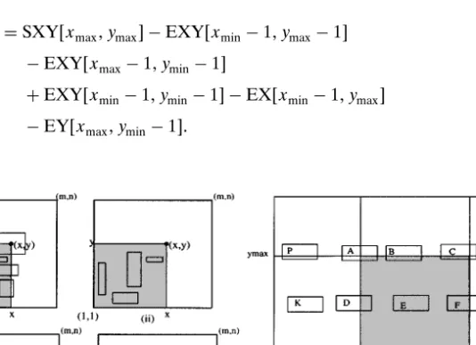
the exact number of bounding boxes in a rectangular region. The proposed method uses four 2D arrays SXY, EXY, EX, EY each of size m × n (see Figure 3(a)). Each bounding box with x-extent xmin; xmax and y-extent ymin; ymax increments both SXYxmin; ymin and EXYxmax; ymax by one. Each bounding box also increments both EXxmax; y and EYx; ymax by one for ymin≤ y ≤ ymax and xmin≤ x ≤ xmax, respectively. These operations correspond to rasterizing the right and top sides of the bounding box for computing its contribution to the EX and EY arrays, respec-tively. After processing all bounding boxes, a 2D prefix-sum operation is performed on both SXY and EXY arrays. In addition, rowwise and columnwise 1D prefix-sum operations are performed on the EX and EY arrays, respectively. After the prefix-sum operations on the arrays, SXYx; y gives the number of bounding boxes intersecting the region 1; 1y x; y. In other words, it finds the number of bound-ing boxes that start (or whose lower-left corners reside) in that region. EXYx; y gives the number of bounding boxes that end (whose upper-right corners reside) in the region 1; 1y x; y. EXx; y gives the number of bounding boxes whose right sides intersect the line segment 1; y; x; y. EYx; y gives the number of bounding boxes whose top sides intersect the line x; 1; x; y.
After defining the arrays SXY, EXY, EX and EY, we can calculate the exact bb-count (WL) of a region xmin; yminy xmax; ymax as follows;
WL = SXYxmax; ymax − EXYxmin− 1; ymax− 1 − EXYxmax− 1; ymin− 1
+ EXYxmin− 1; ymin− 1 − EXxmin− 1; ymax
− EYxmax; ymin− 1: [4]
Figure 3. (a) The 2D arrays used for the exact model: (i) SXY, (ii) EXY, (iii) EX, and (iv) EY. (b) The
As seen in Eq. 4, the proposed scheme requires only 4 subtractions and 1 ad-dition to query the exact bb-count of a rectangular region. The correctness of Eq. 4 can easily be verified with the help of Fig. 3(b) as follows. Each letter (A − P) in the figure represents the bounding boxes of the same type. The ex-act bb-count of the shaded rectangular region is equal to the number of bound-ing boxes of types A − I. SXYxmax; ymax gives the number of bounding boxes of types A − P. EXYxmin− 1; ymax− 1 gives the number of bounding boxes of types J; K; L and EXYxmax− 1; ymin− 1 gives the number of bounding boxes of types L; M; N. Since we subtract the number of L-type bounding boxes twice, we add EXYxmin− 1; ymin− 1 to the sum. Arrays SXY and EXY are not sufficient for the exact computation because of the bounding boxes of types O and P. So, we use EXxmin− 1; ymax and EYxmax; ymin− 1 to subtract the number of bounding
boxes of types P and O, respectively. 6. Screen decomposition algorithms
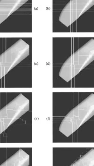
In this section, we present P-way image-space decomposition algorithms according to the taxonomy given in Section 4. Here P denotes the number of processors. Example 16-way decompositions for all decomposition schemes discussed here are displayed in Figure 6.
6.1. 1D decomposition algorithms
The 1D decomposition schemes use 1D arrays with the exact model. Without loss of generality, only horizontal decomposition is discussed here. Note that the horizontal decomposition preserves the intra-scanline coherency which is a valuable asset for the DVR algorithms utilizing such coherency. The load-balancing problem in the decomposition of 1D domains can be modeled as the chains-on-chains partitioning (CCP) problem [2]. In the CCP problem, we are given a chain of work pieces called modules and wish to partition the chain into P subchains, each subchain consisting of consecutive modules. The subchain with the maximum load is called the bottleneck subchain and the load of this subchain is called the bottleneck value of the partition. The objective is to minimize the bottleneck value. In 1D image-space decomposition, the ith module corresponds to the ith scanline and the load Wij of
a subchain i; j corresponds to the bb-count of the respective horizontal stripe. Wij is computed in O1 time by using 1D arrays YS and YE according to Eq. 2.
6.1.1. Heuristic horizontal decomposition (HHD). The screen is decomposed into
P horizontal stripes recursively. At each recursive-bisection step, a region i; j is divided into two regions i; k and k + 1; j such that the horizontal division line k minimizes the expression maxWi; k; Wk+1; j. Although each bisection achieves an
optimal division, the sequence of these optimal bisections may lead to poor load balancing. The HHD algorithm runs in 2M log P time.
6.1.2. Optimal horizontal decomposition (OHD). The existing algorithms for the
optimal solution of the CCP problem can be classified into two categories: dynamic programming and probe-based methods. We use Nicol’s probe-based CCP algo-rithm [21] because of its better speed performance. Nicol’s algoalgo-rithm is based on a
probe function, which takes a candidate bottleneck value L and determines whether
a partition exists with a bottleneck value L0, where L0 ≤ L. The probe function
loads consecutive processors with consecutive subchains in a greedy manner such that each processor is loaded as much as possible without exceeding L. That is, the probe function finds the largest index i1 such that W1; i1 ≤ L by using the binary search. Similarly, it finds the largest index i2 such that W1; i2≤ W1; i1+ L. This pro-cess continues until either all modules are assigned, or some modules remain after loading P parts. In the former case, we say that a partition with a bottleneck value no more than L exists. In the latter case, we know that no partition exists with a bottleneck value less than or equal to L. It is clear that this greedy approach will find a solution with a bottleneck value no greater than L if there is any. The probe function runs in OP log M time.
Nicol’s algorithm exploits the fact that candidate L values all have the form of Wij for 1 ≤ i ≤ j ≤ M. It efficiently searches for the earliest range Wij for which Lopt = Wij by considering each processor in order as a candidate bottleneck processor in an optimal mapping. The algorithm uses the binary search and finds the greatest index i1such that the call of probe with W1; i1 returns false. Here, either W1; i1+1is the bottleneck value of an optimal solution, which means that processor 1 is a bottleneck processor, or W1; i1 is the cost of processor 1 in an optimal solution. We save W1; i1+1 as L1; and starting from i1+ 1 perform the same operation to find i2 and L2. This operation is repeated P times and the minimum of Li values for 1 ≤ i ≤ P constitutes the optimal bottleneck value. Once the optimal bottleneck value is found, the division points for an optimal decomposition can easily be found by using the greedy approach of the probe function. The complexity of this probe-based CCP algorithm is OM + P log M2, where the 2M cost comes from the
initial prefix-sum operation on the YS and YE arrays.
6.2. 2D decomposition algorithms
6.2.1. Rectilinear decomposition (RD). This scheme is a 2D decomposition
algo-rithm using 2D arrays with the exact model. This scheme divides the y-dimension into p horizontal stripes and the x-dimension into q vertical stripes, where p × q = P. We use Nicol’s iterative algorithm [21] that utilizes CCP for rectilinear decom-position. As the optimal rectilinear decomposition is known to be NP-complete [9], this algorithm finds a suboptimal solution.
The iterative algorithm is based on finding an optimal partition in one dimension given a fixed partition in the alternate dimension. The next iteration uses the parti-tion just found in the previous dimension as a fixed partiparti-tion and finds an optimal partition in the other dimension. This operation is repeated, each time fixing the partition in the alternate dimension. The decomposition problem in one dimension
is the adaptation of the CCP problem. It is proven that the iterations converge very fast to a locally optimum solution [21].
The original algorithm has OKn2+ pq log n2-time complexity for an n×n
square coarse mesh, where K is the number of iterations. Here, the 2n2 cost
comes from collapsing stripes into chains. In this work, we use our exact model proposed in Section 5.2.2 to query the bb-count of a rectangular region in O1 time. This scheme avoids the need for collapsing at each iteration, thus reducing the overall complexity to On2+ Kpq log n2. We also note that this asymptotic
improvement proposed for image-space decomposition is also valid for the rectilin-ear decomposition of general 2D workload arrays. In the general case, the n × n workload array should be converted into a SAT by performing a 2D prefix-sum operation in 2n2 time at the beginning.
6.2.2. Jagged decomposition (JD). In the jagged decomposition, the screen is
par-titioned into p horizontal stripes, and each horizontal stripe is independently parti-tioned into q vertical stripes, where p×q=P.
Heuristic Jagged Decomposition (HJD). This algorithm is a 2D decomposition
algorithm using 1D arrays with the exact model. In this scheme, the screen is divided into p horizontal stripes through a recursive-bisection based heuristic as in the HHD scheme using 1D YS and YE arrays. After this 1D decomposition along the y-dimension, the workload distribution in the x-dimension is calculated for each horizontal stripe using two 1D arrays XS and XE. Then, each horizontal stripe is divided independently in parallel into q vertical stripes in the x-dimension using the same recursive-bisection based heuristic. The HJD algorithm runs in 2M log p + N log q time since the vertical partitioning of the horizontal stripes are performed in parallel.
Optimal Jagged Decomposition (OJD). The OJD algorithms presented in this
section are based on the optimal semi-generalized block partitioning algorithm proposed by Manne and Sørevik [17]. Their algorithm extends the dynamic-programming based 1D CCP [16] to OJD. They perform a p-way CCP on the rows of the workload array. The cost of a subchain in a p-way rowwise partition is found by applying a q-way CCP on the columns of that stripe and taking the bottleneck value of the columnwise partition as the cost of the subchain. The complexity of their algorithm is Opqm − pn − q. In this work, we extend Nicol’s probe-based CCP algorithm to OJD of general 2D workload arrays. A straightforward extension of Nicol’s CCP algorithm leads to an Op log m2mn + q log n2-time
OJD algorithm. Fortunately, the run time of our algorithm asymptoticly reduces to Omn + p log m2q log n2 by converting the 2D m × n workload array into
a SAT through an initial 2D prefix-sum operation in 2mn time as mentioned earlier. The details of the proposed OJD algorithm can be found in [13].
The proposed OJD algorithm is exploited in two distinct image-space decom-position schemes, namely OJD with the IAH model (OJD-I) and OJD with the exact model (OJD-E). Note that the OJD-I scheme will create a suboptimal jagged decomposition for actual primitive distribution because of the IAH model used.
6.2.3. Orthogonal recursive bisection (ORB). We present four algorithms based on
the orthogonal recursive bisection paradigm. These algorithms divide a region into two subregions so that the workload of the most heavily loaded subregion is min-imized. Then, they recursively bisect the subregions, each time dividing along the longer dimension, until the number of regions is equal to the number of proces-sors. Dividing the longer dimension aims at reducing the total perimeter of the final regions as an attempt to reduce the amount of primitive replication due to the primitives intersecting multiple regions.
ORB with 1D arrays (ORB-1D). This scheme is a 2D decomposition algorithm
using 1D arrays with the exact model. In this scheme, the primitive distribution over both dimensions of the screen is needed to divide the screen horizontally or vertically. 1D arrays are used for each dimension of the screen. That is, in addition to the YS and YE arrays for the y-dimension, each processor allocates XS and XE arrays for the x-dimension of the screen.
In this scheme, the initially created workload arrays are updated between the successive steps of the decomposition operations. Therefore, the global-sum and prefix-sum operations are repeated after each update of the workload arrays [1]. Initially, each processor is assigned the full screen as its local image region. Each processor divides its local image region into two regions along the longer dimen-sion. Note that for the group of processors that are assigned to the same image region, the division will be the same. After the division, half of the processors are assigned to one of the regions, and the other half of the processors are assigned to the other region. Then, each processor sends the local bounding boxes intersecting the other region to the neighbor processor assigned to that region. Neighborhood between processors can be defined according to various criteria such as intercon-nection topology of the architecture, labeling of the processors etc. In this work, the hypercube labeling is selected for the neighborhood definition since it is very simple. After this exchange operation, each processor has all bounding boxes that project onto its new local screen region and the decomposition operation is repeated for the new image region. In order to decompose the new screen region, we need to update the (X/Y)S and (X/Y)E arrays for the new region. We update these arrays incrementally using the bounding boxes exchanged between the processors. Each processor decrements the appropriate positions in its local (X/Y)S and (X/Y)E ar-rays for each bounding box its sends and increments the appropriate locations in these arrays for each bounding box it receives.
Each recursive-bisection level of the ORB-1D algorithm consists of two phases: subdivision, and bounding-box classification and migration. The overall complexity of the subdivision phase is 2N log P for a square screen of resolution N × N. Un-der average-case conditions, half of the bounding boxes can be assumed to migrate at each recursive-bisection level of the algorithm. Hence, if primitive replication is ignored, the total volume of communication due to the bounding-box migrations will be B/2 log P bounding boxes, where B denotes the total number of bound-ing boxes in the scene. Under perfect load balance conditions, each processor is expected to hold B/P bounding boxes and each processor pair can be assumed to exchange B/2P bounding boxes at each level. Hence, under these conditions,
to-tal concurrent volume of communication will be B/2P log P. Note that primitive replication will increase these values.
ORB with IAH model (ORB-I). This scheme is a 2D decomposition algorithm
using 2D arrays with the IAH model. ORB-I is equivalent to the mesh-based adap-tive hierarchical decomposition scheme (MAHD) proposed by Mueller [20]. The bisection lines for dividing along the longer dimensions are found by using the bi-nary search on the SAT. The ORB-I algorithm runs in 2n√P time for a square coarse mesh of size n × n.
ORB with medians-of-medians (ORBMM). The algorithms presented in this
sec-tion are 2D decomposisec-tion algorithms using 2D arrays with the IAH model. In this scheme, the screen is divided using ORB with the medians-of-medians approach (ORBMM) [23, 27]. The medians-of-medians scheme is used to decrease the load imbalance at each recursive decomposition step by relaxing the straight line restric-tion in the division. We apply ORBMM on a cartesian mesh (ORBMM-M) and a quadtree (ORBMM-Q).
In ORBMM-Q, we generate a quadtree from the mesh superimposed on the screen to decrease the errors due to the IAH model. Each leaf node of the tree is referred to here as a quadnode. The quadtree is generated in such a way that each quadnode has approximately the same workload. The screen is decomposed at the quadnode boundaries. In this work, we use a bottom-up approach to generate a quadtree, whereas a top-down approach was implemented in [11]. That work uses a 2D segment tree [24] to generate the quadtree. The 2D segment tree data structure has a recursive structure. In the top-down approach, the root of the tree covers the full screen and at each level a node is divided into four quadrants forming its children. This division is repeated until the size of a leaf node is equal to one mesh cell. Then, the segment tree is traversed to generate the quadnodes. In the bottom-up approach, we join the mesh cells to form the quadnodes. The mesh cells may be considered as the leaf nodes of the segment tree. In this scheme, we do not explicitly create a segment tree. Instead, we consider a virtual segment tree superimposed on the coarse mesh. This virtual segment tree is traversed in a bottom-up fashion and the quadnodes are inserted into a linked-list structure. In this traversal, if the cost of a node is under a specified threshold value, but one of the siblings exceeds the threshold value, we add this node to the quadnode list. In addition, if four sibling nodes do not individually exceed the threshold value, but their sum exceeds, we add four of them to the quadnode list. The threshold value is selected empirically as a certain percentage of the total number of primitives. Larger threshold values cause poor load balance, whereas smaller values result in more irregular partitions and larger decomposition time.
In ORBMM-M, the cells of the coarse mesh are inserted into a linked-list struc-ture in a similar way to that of ORBMM-Q. This scheme may also be considered as a special case of the quadtree scheme, where the threshold value is zero and each leaf node is inserted into the linked-list structure.
At each recursive-bisection step of ORBMM, the mid-points of the quadnodes are used to find the median line. The problem with this scheme is how to assign the
quadnodes which straddle the median-line. Taking the centers of the quadnodes and assigning them according to their centers may cause load imbalance. The medians-of-medians (MM) scheme [23, 27] is used to alleviate this problem. The idea in the MM scheme is once the median line is determined, the border quadnodes that straddle the median-line are identified and repartitioned. In this phase, we sort the border quadnodes along the bisection direction and assign the nodes in this order to the one side so that the load of the maximally loaded side is minimized. Both ORBMM-Q and ORBMM-M run in On2√P time for a square coarse mesh of
size n × n.
6.2.4. Hilbert-curve based decomposition (HCD). This scheme is a 2D
decomposi-tion algorithm using 2D arrays with the IAH model. In the HCD scheme, the 2D coarse mesh is traversed according to the Hilbert curve to map the 2D coarse mesh to a 1D chain of mesh cells. That is, the mesh cells are assigned to the processors such that each processor gets the cells that are consecutive in this traversal. The load-balancing problem in this decomposition scheme reduces to the CCP problem. The advantage of the Hilbert curve over the other space-filling curves [19, 23] is that it traverses the 2D mesh along neighbor cells without any jumps. Therefore, we may expect that the total perimeter of the resulting regions will be less com-pared to the regions to be obtained by other curves. An example for traversing a 2D mesh with the Hilbert curve is shown in Figure 4(a). The numbers inside the cells represent the order the mesh cells are traversed.
Our approach to traverse the mesh is based on the costzones scheme proposed by Singh et al. [27]. Their approach traverses the 2D segment tree already superim-posed on the space. Here, we superimpose a virtual 2D segment tree on the screen. The key idea in this approach is to traverse the child nodes in a predetermined order such that the traversal of the leaf nodes forms a space-filling curve. As the children of a node are the quadrants of the region represented by that node, we have four possible starting points and two possible directions (clockwise or counter-clockwise) for each starting point. An appropriate choice of four out of the eight orderings is needed. The ordering of the children of a cell C depends on the
order-Figure 4. (a) Traversing a 2D mesh with the Hilbert curve and mapping of the mesh-cell locations into
ing of C’s parent’s children and the position of C in this ordering (Fig. 4(b)). The cells are assigned to the processors during the traversal of the virtual 2D segment tree.
Mapping the 2D coarse mesh to a 1D chain of mesh cells takes 2mn time and the recursive-bisection based heuristic used for load-balanced partitioning takes 2mn log P time.
6.2.5. Graph-partitioning based decomposition (GPD). This scheme is a 2D
de-composition algorithm using 2D arrays with the IAH model. This algorithm models the image-space decomposition problem as a graph-partitioning (GP) problem [12]. Each cell in the coarse mesh is assumed to be connected to its north, south, west and east neighbors. The vertices of the graph are the mesh cells and the concep-tual connections between the neighbor mesh cells form the edges of the graph. The weight of a cell represents the bb-count of the cell. The weight of an edge between two neighbor cells represents the number of bounding boxes intersecting both cells. The objective in GP is to minimize the cutsize among the parts while maintain-ing the balance among the part sizes. Here, the cutsize refers to the sum of the weights of the cut edges, where an edge is said to be cut if its pair of vertices be-long to two different parts. The size of a part refers to the sum of the weights of the vertices in that part. In our case, maintaining the balance among the part sizes corresponds to maintaining the computational load balance. Minimizing the cutsize corresponds to minimizing the amount of primitive replication due to the shared primitives. The state-of-the-art GP tool MeTiS [10] is used in this work. The GP approach decomposes the screen in the most general way. Unlike the pre-vious decomposition algorithms, noncontiguous sets of cells may be assigned to a processor.
In the GPD scheme, each processor tallies the bounding boxes of its local primi-tives to the mesh cells and updates the weights of the corresponding cells and edges. The cell weights are updated using the IAH model. In order to decrease the errors caused by the primitives shared among more than two cells, we adopt the follow-ing scheme for edge weightfollow-ing. First, we classify the shared boundfollow-ing boxes into three categories: vertical, horizontal, and general. The vertical bounding boxes are the ones that intersect multiple cells in only a single column of the coarse mesh. The horizontal bounding boxes intersect multiple cells in only a single row. The general bounding boxes intersect multiple (at least 4) cells in different rows and columns. The weight of an edge between two neighbor cells in a row (column) is incremented by a value proportional to the number of horizontal (vertical) bound-ing boxes intersectbound-ing those two cells. The weight of an edge between two neigh-bor cells is incremented by each general bounding box intersecting those two cells with a value inversely proportional to the total number of cells the bounding box intersects.
The average-case running time of recursive-bisection based pMeTiS can be as-sumed to be Oe log P, where e denotes the number of edges in the given graph. Since the graph constructed in the GPD scheme contains 4mn − 2m + n edges, the GPD algorithm runs in Omn log P. However, the hidden constants in the com-plexity are substantially larger than those of the other decomposition algorithms.
7. Primitive redistribution
After the decomposition of the screen, each processor needs all the primitives inter-secting the region it is assigned in order to perform the local rendering calculations. Thus, the local primitives in each processor should be redistributed according to the region-to-processor assignment. Each processor classifies its local primitives accord-ing to the regions they intersect. Accordaccord-ing to the classification, each primitive is stored in the respective send buffer of that region. If a primitive overlaps multiple regions, the primitive is stored in the send buffers of the respective regions. These buffers are exchanged to complete the redistribution of the primitives. In this work, we propose several algorithms for classifying primitives in the redistribution phase.
7.1. 2D mesh-based primitive classification
This is the most general classification scheme applicable to all decomposition schemes. In this scheme, each mesh cell constituting a pixel block is marked with the index of the processor whose screen region covers this particular cell. Then, each bounding box is tallied to the mesh cells, and the respective primitive is stored into the send buffers of the processors according to the marks of the cells the bounding box covers. This scheme is computationally expensive since it involves tallying the bounding boxes, and its complexity per primitive is proportional to the area of the bounding box of the primitive. This scheme is adopted in the HCD, ORBMM-Q, ORBMM-M and GPD algorithms, since these algorithms produce non-rectangular regions.
7.2. Rectangle-intersection based primitive classification
The expensive tallying operation needed in the mesh-based classification can be avoided for the decomposition algorithms that generate rectangular regions. The intersection of a primitive with a rectangular region can easily be tested at a very low cost by testing the intersection of both the x and y extents of the primitive with the x and y extents of the region, respectively. This classification scheme is adopted in the ORB-1D and ORB-I decomposition algorithms that generate rectangular regions in a hierarchical manner based on recursive bisection. The hierarchical nature of these two decomposition schemes is exploited to reduce the number of intersection tests for a bounding-box b to ORblog P, where Rb denotes number of regions intersecting b.
7.3. Inverse-mapping based primitive classification
We propose more efficient algorithms for the 1D horizontal, 2D rectilinear and 2D jagged decomposition schemes by exploiting the regularity of the resulting de-compositions. In these schemes, it is possible to give numbers to the resulting re-gions in row-major (column-major) order if the screen is divided completely in the
y-dimension (x-dimension). For example, in the row-major ordering of a p × q rec-tilinear decomposition, the region at the rth horizontal stripe and cth vertical stripe is labeled as qr − 1 + c for r = 1; : : : ; p and c = 1; : : : ; q.
In the 1D decomposition schemes, we use an inverse-mapping array IMY of size m. This array represents the assignment of the scanlines to the processors. That is, IMYi = k for each scanline i in the kth horizontal stripe. Then, a primitive with y-extent ymin; ymax is inserted into the send buffer of each processor k for IMYymin ≤ k ≤ IMYymax. This algorithm is faster than the rectangle-intersection based scheme, because only two simple table lookups are sufficient to classify a primitive.
The rectilinear decomposition scheme requires two inverse-mapping arrays: IMY of size m and IMX of size n. Arrays IMY and IMX represent the assignments of the rows (scanlines) and columns of the screen to the horizontal and vertical stripes of the decomposition. That is, IMYi = r for each row i of the screen in the rth horizontal stripe. Similarly, IMXj = c for each column j of the screen in the cth vertical stripe. A primitive with y-extent ymin; ymax and x-extent xmin; xmax is inserted into the send buffer of each processor k = qr − 1+c for IMYymin ≤ r ≤ IMYymax and IMXxmin ≤ c ≤ IMXxmax. This scheme requires only 4 table lookups for the classification of a primitive.
The jagged decomposition scheme requires p + 1 inverse-mapping arrays. One array IMY of size m is needed for the horizontal striping and one IMXr array
of size n is needed for the vertical striping in the rth horizontal stripe for r = 1; : : : ; p. Here, IMYi = r for each row i of the screen in the rth horizontal stripe. IMXrj = c for each column j in the cth vertical stripe of the rth horizontal
stripe. A primitive is inserted into the send buffer of each processor k = qr − 1+c for IMYymin ≤ r ≤ IMYymax and IMXrxmin ≤ c ≤ IMXrxmax. This
scheme requires 2h + 2 table lookups for classifying a primitive which intersects h consecutive horizontal stripes.
8. Models for performance comparison
The performance comparison of the image-space decomposition algorithms is conducted on a common framework according to three criteria: load balancing, amount of primitive replication and parallel execution time. Primitive replication is a crucial criterion because of the following reasons. A primitive shared by k pro-cessors incurs k−1 replications of the primitive after the redistribution. Thus, each replication of a primitive incurs the communication of the primitive during the re-distribution phase, and redundant computation and redundant storage in the local rendering phase. Furthermore, as we will discuss in Section 8.2, primitive replica-tion has an adverse effect on the load balancing performance of the decomposireplica-tion algorithms. The parallel execution time of a decomposition algorithm is also an im-portant criterion since the decomposition operation is a preprocessing for the sake of efficient parallel rendering.
A formal approach for the prediction, analysis and comparison of the load bal-ancing and primitive replication performances of the algorithms requires a
prob-abilistic model. However, such a formal approach necessitates the selection of a proper probabilistic distribution function for representing both the bounding-box and bounding-box size distribution over the screen. In this work, we present a rather informal performance comparison based on establishing appropriate qual-ity measures. The experimental results given in Section 9 confirm the validqual-ity of the proposed measures.
8.1. Primitive replication
Among all decomposition algorithms, only the GPD algorithm explicitly tries to minimize the amount of primitive replication. In the other algorithms, the topologi-cal properties of the underlying decomposition scheme have a very strong effect on the amount of primitive replication. Here, we establish two topological quality mea-sures: the total perimeter of the regions and the total number of junction points generated with the division lines.
The number of bounding boxes intersecting two neighbor regions is expected to increase with increasing length of the boundary between those two regions. In the 1D decomposition schemes, the total perimeter is equal to P − 1N. In both jagged and rectilinear decomposition schemes, the total perimeter is equal to p − 1N + q − 1M for a p × q processor mesh. For an N × N square screen, the total perimeter is minimized by choosing p and q such that the resulting p × q pro-cessor mesh is close to a square as much as possible. The total perimeter becomes 2√P − 1N for a√P ×√P square processor mesh in both jagged and rectilinear decomposition schemes. In the ORB and ORBMM decomposition schemes for P being an even power of 2, the total perimeter values are equal to 2√P − 1N and 2√P − 1N + P − 1N/n, respectively, if the successive divisions are always per-formed along the alternate dimensions. Note that the total perimeter of ORB with divisions along the alternate dimensions is equal to that of the jagged and rectilin-ear schemes. However, in our implementation for the ORB and ORBMM schemes, dividing along the longer dimension is expected to further reduce the total perime-ter especially in the decomposition of highly non-uniform workload arrays for large P values. In the HCD scheme, using the Hilbert curve as the space-filling curve is an implicit effort towards reducing the total perimeter since the Hilbert curve avoids jumps during the traversal of the 2D coarse mesh. Nevertheless, the total perime-ter in the HCD scheme is expected to be much higher than those of the other 2D decomposition schemes, since HCD generates irregularly shaped regions.
The total perimeter measure mainly accounts for the amount of replication due to the bounding boxes intersecting two neighbor regions under the assumption that both x and y extents of the bounding boxes are much smaller than the x and y ex-tents of the regions respectively. A junction point of degree d > 2—shared by the boundaries of d regions—is very likely to incur bounding boxes intersecting those d regions thus resulting in d − 1 replications of the respective primitives. Each junc-tion point can be weighted by its degree minus one so that the sum of the weights of the junction points can be used as a secondary quality measure for the relative performance evaluation of the 2D decomposition schemes. It should be noted here
that the validity of this measure depends on the assumption that the bounding boxes are sufficiently small and the junction points are sufficiently away from each other so that the bounding boxes do not cover multiple junction points. Both jagged and ORB decomposition schemes generate 2p − 1q − 1 junction points each with a degree of 3 for a p × q processor mesh. Here, we assume that the successive di-visions are always performed along the alternate dimensions in the ORB scheme. The number of junction points generated by the rectilinear decomposition scheme is half as much as that of the jagged and ORB schemes. However, each junction point in the rectilinear decomposition scheme has a degree of 4. As seen in Table 2, under the given assumptions and the additional assumption that the bounding-box density remains the same around the junction points, the rectilinear decomposition is expected to incur 25% less primitive replication than both jagged and ORB de-composition schemes due to the bounding boxes intersecting more than two regions. As seen in Table 2, according to the total perimeter measure, the 2D decompo-sition schemes are expected to perform better than the 1D schemes such that this performance gap is also expected to increase rapidly with increasing P. Among the 2D decomposition schemes, the jagged, rectilinear and ORB schemes are expected to display comparable performance. However, ORB can be expected to perform slightly better than the other two schemes because of the possibility of further re-duction in the total perimeter by performing divisions along the longer dimension. As the jagged and rectilinear decomposition schemes are expected to display similar performance according to the total perimeter measure, the rectilinear decomposi-tion scheme is expected to perform better than the jagged decomposidecomposi-tion scheme because of the secondary quality measure.
8.2. Load balancing
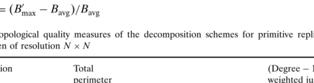
The load-balancing performance of the decomposition algorithms are evaluated according to the actual load-imbalance values defined as
LI = B0
max− Bavg/Bavg [5]
Table 2. Topological quality measures of the decomposition schemes for primitive replication for a
square screen of resolution N × N
Decomposition Total (Degree − 1)
scheme perimeter weighted junction sum
1D (Horizontal) P − 1N 0
Rectilinear 2√P − 1N 3√P − 12
Jagged 2√P − 1N 4√P − 12
ORB ≤ 2√P − 1N 4√P − 12
ORBMM ≤ 2√P − 1N + P − 1N/n 4√P − 12
P is assumed to be an even power of 2 for 2D decomposition schemes. A square coarse mesh of resolution n × n is assumed for the 2D-2D algorithms, so that N/n denotes the height and width of a coarse-mesh cell.