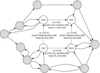
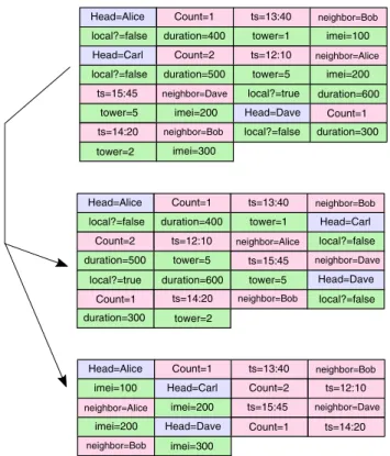
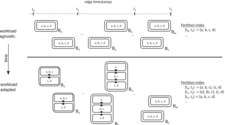
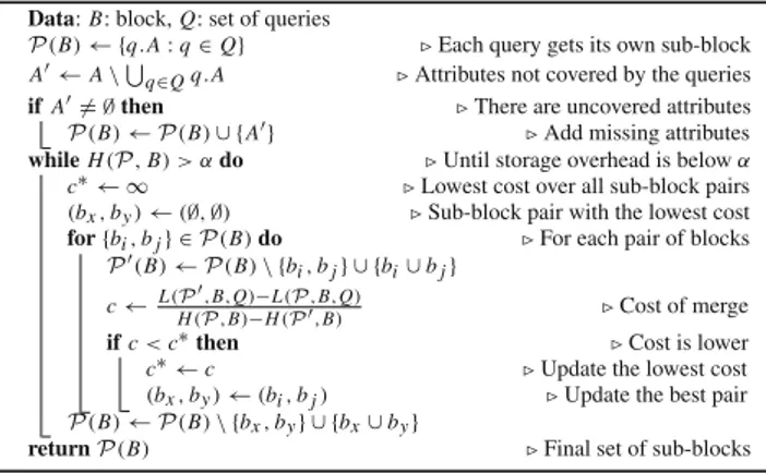
RailwayDB: adaptive storage of interaction graphs

According to Charles Jencks (2006), the iconic building shares certain aspects both with an iconic object, such as Byzantine painting of Jesus, and the

Since the present study aims at exploring whether using a wordlist in the class through a word wall is an effective vocabulary learning strategy to improve their repertoire of

The so-called social sciences (at the time Dewey writes about them), for example, remain embedded in judgments based on moral preconceptions that reflect and impose cultural

Yaratıcılığın iyilikle el ele gitmediğini epey önce öğrendim ama Attilâ Ilhan'ın iyi insan olması, taşıdığım bu yükün pahasını çok arttırdı.. Aklıma sık

This research aimed to determine the knowledge, attitudes, opinions and application among students from the departments of nursing, midwifery, and dietetics of the Faculty of

Yalı köyünün, meş­ hur çayırın kenarından geçilip sağa sapılır; bir müddet gittik­ ten sonra yine sağa çarh edilip iki tarafı çınarlarla sıralanmış

In addition to urban effects on rural areas, cities also developed by enlarging and sprawling on rural areas, destroyed agricultural lands which are vitally

Saptanan ortak temalardan yola çıkarak sosyal bilimler eğitiminde ölçme ve değerlendirmeye dair problemlerin; hem içinde bulunduğumuz acil uzaktan eğitim süreci