Metaheuristics for the permutation flow shop problems

(1)

GRADUATE SCHOOL OF NATURAL AND APPLIED SCIENCES

PhD THESIS

Metaheuristics for the Permutation Flow Shop Problems

Thesis Advisor: Assist. Prof. Dr. Korhan KARABULUT

Co-Department of Computer Engineering

Presentation Date: 29.01.2016

Bornova-2016

(2)

(3)

ABSTRACT

Metaheuristics for the Permutation Flow Shop Problems

PhD in Computer Engineering

Supervisor: Assist. Prof. Dr. Korhan KARABULUT

Co-January 2016, 120 pages

In this study, two variants of permutation flow shop scheduling problem with sequence dependent setup times are considered. The first problem studied in this thesis is the permutation flow shop problem with sequence dependent setup times under makespan criterion. A new iterated greedy algorithm and a new local search algorithm is developed for this problem. The new local search includes insertion neighborhood and swap neighborhood. A new speed up technique is developed to reduce the cost of the swap neighborhood search, which is inspired -known speed-up method for the insertion neighborhood. The developed speed up technique can save fifty percent CPU time in average. The developed iterated greedy algorithm utilizing the new swap speed-up method is tested on the benchmark instances from the literature and new best-known solutions are found for 250 out of 480 problem instances. The second problem considered is the permutation flow shop scheduling problem with sequence dependent setup times under total flow time criterion. This problem is studied for the first time in the literature to best of our knowledge. NEH_EDD and LR heuristics as well as speed-up methods for problems without the sequence dependent setup times for insertion and swap neighborhoods are adapted to this problem. Several metaheuristics are developed and executed on a benchmark set. The performances of the developed algorithms are compared and the results are presented.

Keywords Sequence-dependent setup times, flow shop scheduling problem,

metaheuristics, iterated greedy algorithm, variable neighborhood search,

(4)

Meta-Sezgisel Algoritmalar Ocak 2016, 120 sayfa Bu tezde, . olarak s tamamlanma

nin en iyilenmesi Bu problem

algoritma ve yeni . Yeni yerel arama

azalta

esinlenerek bu

i hesaplan ni

ortalama olarak elli .

0 tanesi kinci

olarak

bu problem ilk defa NEH_DD ve LR sezgisel

. Bir

. .

(5)

Anahtar Kelimeler - tipi izelgeleme problemi, yenilemeli

(6)

ACKNOWLEDGEMENTS

I am grateful to my supervisor, Assist. Prof. Dr. Korhan KARABULUT and

co-supervisor, , for their endless support. I

am thankful for their various ideas, suggestions and for all of their encouraging words in the moments of adversity.

And I would like to thank to Assist. Prof. Dr. for

his support and advices during the thesis progress meetings.

And I want to than

Finally, I thank my family for their constant encouragement and motivation during my studies.

(7)

TEXT OF OATH

s for The Permutation Flow S

written without applying to any assistance inconsistent with scientific ethics and traditions, that all sources from which I have benefited are listed in the bibliography, and that I have benefited from these sources by means of making references.

(8)

INDEX OF FIGURES

Figure 1-1 A classification of scheduling problems (Dhingra, 2012) 5

Figure 1-2 Gantt chart for a sample schedule for sample instance 6

Figure 1-3 Gantt chart for a sample schedule for Ta001 instance 6

Figure 1-4 Gantt chart of a sample schedule for Ta001 instance with SDST 9

Figure 3-1 : Swapping job 3 with job 5 25

Figure 3-2 Total Flowtime Insertion operation of job 5 30

Figure 3-3 Total Flowtime swap of job 4 and job 7 31

Figure 4-1 A one-dimensional state-space landscape in which elevation

corresponds to the objective function (Russell & Norvig, 2010) 35

Figure 4-2 Pseudocode of the NEH algorithm 36

Figure 4-3 Iterated Greedy Algorithm pseudo code 38

Figure 4-4 Iterative Improvement procedure using insertion neighborhood 39

Figure 4-5 Basic VNS Algorithm 40

Figure 4-6 VNS using different neighborhoods 41

Figure 4-7 Pseudocode of the VND algorithm 41

Figure 4-8 Pseudocode for GVNS algorithm 42

Figure 5-1 Interaction Plot of Factor X and Factor Y 46

(12)

Figure 6-1 The proposed IG_IJ algorithm 49

Figure 6-2 Local Search algorithm used in IG_IJ 50

Figure 6-3 The pseudo code of the proposed IG_VNS algorithms 52

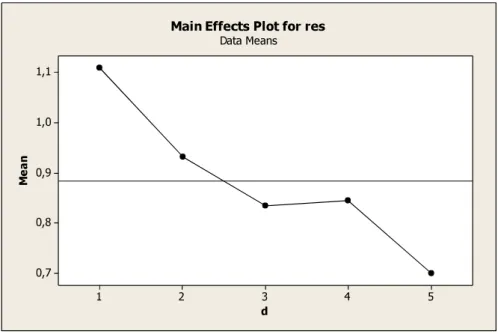
Figure 6-4 Main effect plots of parameters 54

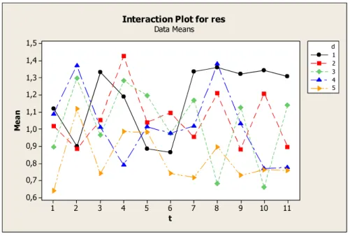
Figure 6-5 Interaction plot for destruction size versus jumping probability 55

Figure 6-6 Interaction plot for destruction size versus temperature adjustment

parameter 56

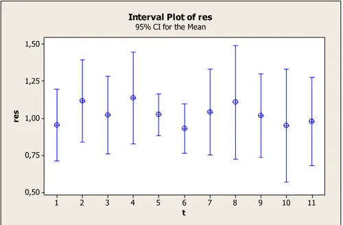
Figure 6-7 Interval Plot of (jumping probability) 57

Figure 6-8 Interval Plot of size 57

Figure 6-9 VLSRCTalgorithm 59

Figure 6-10. The proposed IG_VLSIKTalgorithm 60

Figure 6-11 Main effect plots of d size for IG_RS algorithm 62

Figure 6-12 Main effect plots of temperature adjustment parameter for IG_RS

algorithm 62

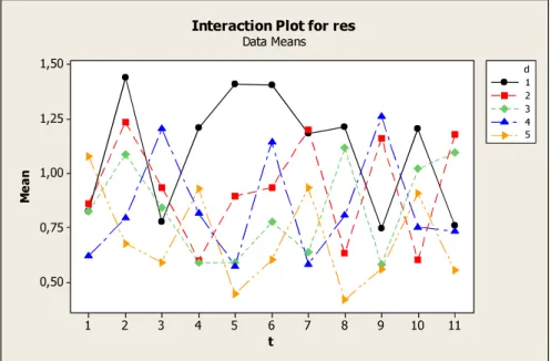
Figure 6-13. Interaction plot of temperature adjustment parameter and destruction

size for IG_RS algorithm 63

Figure 6-14 Interval plot of d size for IG_RS algorithm 64

Figure 6-15 Interval plot of temperature adjustment parameter for IG_RS

algorithm 64

(13)

Figure 6-17 Main effect plots of temperature adjustment parameter for

IG_VLSRCTalgorithm 65

Figure 6-18 Interaction plot of temperature adjustment parameter and destruction

size for IG_VLSRCTalgorithm 66

Figure 6-19. Interval plot of d size for IG_VLSRCTalgorithm 67

Figure 6-20. Interval plot of t size for IG_VLSRCTalgorithm 67

Figure 6-21. Main effect plots of d size for IG_VLSIKT algorithm 68

Figure 6-22 Main effect plots of t for IG_VLSIKT algorithm 68

Figure 6-23 Interaction plot of temperature adjustment parameter and destruction

size for IG_VLSIKTalgorithm 69

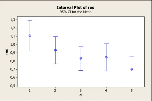
Figure 6-24 Interval plot of destruction size for IG_VLSIKTalgorithm 70

Figure 6-25 Interval plot of temperature adjustment parameter for IG_VLSIKT

algorithm 70

Figure 7-1 Plot of average percentage deviations for SDST10 instances 76

Figure 7-5 Plot of average percentage deviations for SDST10 instances with t=90 78

Figure 7-6 Plot of average percentage deviations for SDST50 instances with t=90 79

(14)

Figure 7-7 Plot of average percentage deviations for SDST100 instances with

t=90 79

Figure 7-8 Plot of average percentage deviations for SDST125 instances with

t=90 80

Figure 7-9 Interval plot of algorithms for t=30 81

Figure 7-10 Interval plot of algorithms for t=60 81

Figure 7-16 Plot of average percentage deviations of algorithms for SDST10

instances with t=90 89

Figure 7-17 Plot of average percentage deviations of algorithms for SDST50 with

t=90 90

with t=90 90

with t=90 91

(15)

Figure 7-23 Plot of average percentage deviations of IG_RSLS and IG_VLSIKS

algorithms for original Taillard instances with t=60 95

Figure 7-24 Plot of average percentage deviations of IG_RSLS and IG_VLSIKS

algorithms for original Taillard instances with t=90 95

Figure 7-25 Interval plot of algorithms for original Taillard instance with t=60 and

(16)

INDEX OF TABLES

Table 3-1. The processing times matrix 26

Table 3-2. The setup times matrix for machine 1 26

Table 3-7. matrix for permutation 28

Table 3-10. Calculation of final makespan value 29

Table 3-11 Completion times matrix for 31

Table 3-12 Completion times matrix for first three jobs 31

Table 3-13 The new finishing times matrix 32

Table 5-1 Two factor factorial design - First example 45

Table 5-2 Two factor Factorial design - Second example 47

Table 6-1 ANOVA table of IG_IJLS 55

(17)

Table 6-3 ANOVA table for IG_VLSRCT 66

Table 6-4 ANOVA table for IG_VLSIKT 69

Table 7-1. The impact of the speed-up method on CPU times on SDST125

instances 72

Table 7-2 Average relative percentage deviations for SDST10 and SDST50

instances 74

instances 75

instances 84

instances 85

Table 7-6 Average relative percentage deviations of IG_RSLS and VLSIKT

(18)

INDEX OF SYMBOLS AND ABBREVIATIONS

Symbols Explanations

Makespan

Permutation of jobs

machine permutation flowshop

makespan minimization problem with sequence dependent setup times

jobs, total number of jobs

machines, total number of machines

starting time of jobs on machine

the starting time of th _{job on} th

machine in forward calculation matrix

Sequence dependent set up time of th

job on th machine where is the

previous job completed on th_machine

machine permutation flowshop total flowtime minimization problem with sequence dependent setup times

the starting time of th job on th

(19)

matrix

the finishing time th job on th

machine in final calculation matrix

Abbreviations

ARPD Average Relative Percentage

Deviation

FJSRA Fictitious Job Setup Ranking

Algorithm

GA Genetic Algorithm

GRASP Greedy Randomized Adaptive Search

Procedure

IG Iterated Greedy

LIT Less Idle Times

LS Local Search

NEH Nawaz, Enscore, Ham Heuristic

NP Non-deterministic Polynomial-time

PFSP Permutation Flowshop Problem

(20)

SPD Smallest Process Distance

SRA Setup Ranking Algorithm

VLS Variable Local Search

VND Variable Neighborhood Descent

VNS Variable Neighborhood Search

(21)

1. INTRODUCTION

Scheduling is determining the order of the jobs to be handled on machines. A schedule can be considered as a plan for the execution of jobs on machines. Efficient scheduling is very important for production and manufacturing. Benefits of an efficient schedule can be increased resource utilization and production process efficiency, reduced inventory and more accurate handling of due dates. Characteristics of the jobs such as their sizes and routes through machines greatly influence the result of the scheduling process. Also all technological constraints should be considered for a feasible schedule. According to Wight (1984), there are two important decision criteria for manufacturing system scheduling; which are

. These are the answers for two questions

? Cox et al. (1992) define scheduling as the actual assignment of starting and/or completion dates to operations or groups of operations to show when these must be done if the manufacturing order is to be completed on d a type of bar chart for illustrating job schedules in 1910s, which is called as a Gantt chart. Even today, Gantt charts are widely used for presenting the schedules. In the early years, the term scheduling was only used for scheduling of the manufacturing systems. Now, scheduling is also very important for non-manufacturing areas.

Fundamental structure in scheduling is generally called as jobs and this term is also used for non-manufacturing environments. Jobs may consist of one or more tasks. The main problem in scheduling is to determine the order of the tasks according the priorities and availability of the resources. Scheduling can be considered as decision-making process of ordering the tasks according to some constraints in order to optimize one or more criteria. For manufacturing systems, scheduling plays an important role in production planning. Better scheduling allows to use the production environment more efficiently and to make better resource allocation.

(22)

Nowadays, fast growing markets and manufacturing systems deal with higher customer expectations in terms of quality of the product, cost of the product and finally its arrival time. Satisfying these conditions is getting harder each day with the increasing customer demands. To catch up with current situation, manufacturing enterprises focus on two main issues. The first issue is using more technological production lines for increasing the production rate and lowering the production time. Also new technologies are important for producing more reliable products with lower unit costs. Flexibility is another important production requirement for the market in order to make changes fast enough to catch up with custo

Second issue is adopting a more utilized production structure that respects resource utilization, inventory costs, and production and manufacturing times. Under these circumstances, manufacturers spend their efforts on achieving production goals that are best for themselves and customers. As it is mentioned above, these goals are also important for non-manufacturing markets or industries.

Scheduling is considered as a decision-making process regarding the current situation of the system. It tries to optimize the system with respect to one or more objectives considering the state of the resources. Resources can be crew in an airport, nurses in a hospital or production components in production lines. Tasks of the operations may differ with the scheduling environment or industry. Schedules also might have different objectives to satisfy the needs and demands; in order to increase the production utility, the objective can be obtaining minimum make span, while in order to minimize the inventory, the objective can be minimizing total flow time or in order to catch the specific production time, the objective can be minimizing tardiness. Inadequate scheduling causes inefficient utilization of production facilities and employees. Moreover, it increases the idle time in production. As a result, this will increase the costs.

1.1 Classification of Scheduling Problems

Scheduling is the process of finding a feasible order for processing in order to optimize the production or system. In 1981, Graves classified the scheduling

(23)

problems and put them into three main and two additional categories. In 2012, Dhingra summarized these categories as follows:

Requirement generation Processing complexity Scheduling criteria Parameter variability Scheduling environment

In the first category, jobs are categorized by their stocking attribute. If orders are not stocked and produced with demand of the customer, this kind of jobs are there is no inventory in this kind of scheduling. In closed shops, production is not only going to be determined by customer demands, it will also produce inventory after production. For closed shop type problems, host sequencing problem and lot-sizing decision has to be made for current inventory. Job shop and flow shop problems are considered in closed shop category. Scheduling problems can also be divided into categories by their processing complexity as follows (Graves,1981):

One-stage, one processor (facility) One-stage, parallel processors (facilities) Multistage, flow shop

Multistage, job shop

In single machine problems, there is only one processing step. All jobs have only one non-repeated task to be processed on the single machine. One stage, parallel processors can be described similar to single machine parallel shops. Again, all jobs have a single task but this single task can be processed on parallel machines. This means, two or more jobs can be processed at the same time (on different machines) in parallel machine systems. In multistage problems, each job has more than one task to be processed on different facilities or machines. Flow shop problem is a special case

(24)

of the multistage problems in which all tasks in all jobs follow the same order through each facility or machine. In the more general case of the multistage problem, named as job shop problem, again all jobs have more than one operation to be processed on the machines but each job has a different operation order (route) through the machines.

The third classification category for the scheduling problems is the scheduling objective according to Graves (1981). In this scheme, scheduling problems are classified according to their schedule cost and schedule performance. Schedule cost includes all expenses for production such as production setup or changeovers in inventory holding cost, etc. Performance of the schedule gives information about optimization criteria, which is the objective for the current state of the system. These performance measures can be utilization of the production lines, in other words minimizing the makespan of the schedule, total completion time of all jobs named as total flow time or average or maximum tardiness with respect to the due dates of the products.

There are two more schemes that can be used for classification of scheduling problems: parameter variability and scheduling environment. In parameter variability, scheduling problems can be divided into two groups as deterministic and stochastic schedules. In scheduling environment, schedules can be categorized as static and dynamic schedules. In static schedules, all requirements are fully specified before the scheduling process and no additional requirements will be added to problem set later. Most of the scheduling problems are deterministic and static. A classification of the scheduling problems is given in Figure 1-1.

(25)

Figure 1-1 A classification of scheduling problems (Dhingra, 2012)

1.2 Permutation Flow Shop Problem

Scheduling problems are keeping their popularity since 1950s when the first seminal publications (Smith, 1956), (Johnson S. , 1954) (Jackson, 1955) began to appear. There are various kinds of scheduling problems that are being studied since. The most general scheduling problem is the job shop scheduling problem. In job shop scheduling problem, there is a finite set of jobs and these jobs consist of ordered operations. There are machines and each can handle at most one operation at a time. Each operation is processed on the machines without interruption. Main purpose is to find a schedule, which optimizes a chosen objective. For job shop scheduling problem there are possible sequences. Gantt chart of a sample schedule for abz06 instance is shown in Figure 1-2.

(26)

Figure 1-2 Gantt chart for a sample schedule for sample instance

Flow shop scheduling problem is one of the most popular scheduling problems. Permutation flow shop problem is a special kind of job shop problem in which all jobs visit each machine in the same sequence. Several criteria can be used to consider the performance of the decision making problem for scheduling, such as makespan which deals with maximum completion time of jobs in all machines, total tardiness which deals with tardiness of the jobs in all machines and total flow time which deals with minimizing inventory costs. Makespan criteria is important for machine utilization (Pan & Ruiz, 2013), while flow time criteria focuses on minimizing the in-process in reserves (Dipak & Sarin, 2008), and tardiness criteria satisfies the customer due dates as a hard deadline constraint (VictorFernandez-Viagas, 2015). There are possible sequences for jobs in permutation flow shop problem. Gantt chart of a sample schedule for Ta001 instance is shown in Figure 1-3.

(27)

1.3 Set up time and Sequence Dependent Set up Time

In real life, preparation of the production environment (changing the operator controls for new parts, cleaning up the production line for new order, adjusting the production line etc.) takes some time, which is called as set up time. Changing the blades for new paper size or preparing the paint tank for new color production can be considered as real life examples. Actually, most of the production systems that deal with different kinds of products need such setup times in order to make some adjustments for the new piece of product. In some cases, the time spent on adjusting the production line or cleaning up the production environment may show differences with respect to job order to be processed on the machine. For example, in paint production, it takes more time to produce white color paint in a tank which was already used for black color paint production, than producing a dark blue color paint in the same tank. In the former case, in addition to required setup time, more water will be needed to wash the tank. If the setup time changes with respect to the previous task that was executed on the machine and the next task that will be executed, then this kind of setup time is called as sequence dependent set up time.

Sequence dependent setup times have significant importance for the production

systems. Luh et al. (1998) ed switchgears

(GIS). In this study, it is reported that model performance in handling of the sequence dependent setup time has a critical effect. As Pinedo (2008) mentions, machine efficiency can be improved up to 20% with correctly handling the sequence dependent set up times in flow shop problems. There is more research on the effect of the sequence set up times in production such as Yi and Wang (2003) and Gendreaua et al. (2001) that showed the significance (impact) of sequence dependent set up times in different cases.

Setup time means preparation of the machine in order to start production and it includes the time needed for setting up the environment, adjusting the system etc. (Allahverdi et.al, 1999). In some applications, this setup time is added to the processing time and neglected. When dealing with separate set up times, two kinds of

(28)

setup times can be seen in the literature. In the first kind, the job type determines the setup time, so it can be named as sequence-independent setup time. In the second kind, both job and machine determines the setup time, so this can be named as sequence dependent set-up (Allahverdi et.al, 1999).

Permutation flow shop scheduling problem with sequence dependent setup time (PFSP - SDST), is also be named as the sequence-dependent setup time flow shop scheduling problem (SDST - FSP) in the literature. In SDST - FSP, setup times (costs) are processed separately instead of being added to processing times of the jobs. While the permutation flow shop problem is popular among researchers, sequence dependent setup time version of the problem has not been studied much. However, set up times have significant effects as shown by many researchers. Wilbrecht and Prescott (1969) showed that SDST has a reasonably large amount of effect when the system operates near the limits.

Maximizing throughput is one of the important goals of scheduling. High utilization and high throughput can be achieved by achieving the optimum makespan schedule for the machines. So, machines will have less idle time and this will lead to higher equipment efficiency.

Flow time can be described as the time consumed by the processes (jobs) on machines. Minimizing the flow time as a scheduling criteria makes fewer inventories for the system and minimizes the mean number of processes (jobs) in the system (Baker & Trietsch, 2009) . In addition, minimum flow time values lead to less cycle time for manufacturing (Ciavotta, Minella, & Ruiz, 2010).

(29)

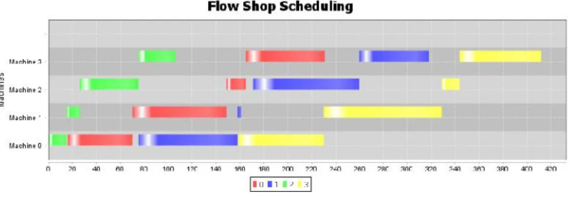
Figure 1-4 Gantt chart of a sample schedule for Ta001 instance with SDST

Gantt chart of a sample schedule for T with large sequence dependent setup times is shown in Figure 1-4. The effect of the sequence dependent setup time is obvious when Figure 1-3 and Figure 1-4 are compared. Figure 1-3 shows the Gantt chart of the same instance without sequence dependent setup times. As observed from Figure 1-4, the total completion of all of the operations has been delayed from 1300 to 2050 when the setup times are considered.

1.4 Scope of the Work

In this thesis; metaheuristic approaches for permutation flow shop problem with sequence dependent set up times have been studied. Two different optimization criteria are considered. The first optimization criterion is the minimization of make span. A novel speedup method for the swap neighborhood is developed for this problem. The proposed speedup method is inspired from the

well-speedup method for the insertion neighborhood. A new iterated greedy (IG) algorithm with a local search procedure that utilizes the developed speed up calculation technique for swap neighborhood in addition to insertion neighborhood is developed. The developed IG algorithm is compared to other metaheuristics from the literature.

The second optimization objective considered in the thesis is total flow time minimization for permutation flow shop problem with sequence dependent set up times. For this problem, (Li, Wang, & Wu, 2009) speed-up calculation method as well as NEH_EDD and LR heuristics are adapted to consider the sequence

(30)

dependent set up times and new local search algorithms are proposed. Experiments are carried out in order to tune the parameters of the implemented metaheuristics. The results of the performances of all implemented algorithms are presented in computational results section and new local minimum values that are obtained by proposed methods are given in appendices.

1.5 Organization of the Thesis

The rest of this thesis is organized as follows: in the second chapter, formal problem descriptions and literature review for the permutation flow shop problem for make span and total flow time criteria are presented. Details of the developed

speed-speed-up method (Li, Wang, & Wu, 2009) are given in chapter 3 along with examples. In chapter 4, heuristic and metaheuristic methods that are used in this thesis are explained. Chapter 5 gives brief information about the design of experiments method. Chapter 6 gives the details of the algorithms that are developed in this thesis along with the details of the design of experiment approach used for tuning the algorithm parameters. In chapter 7, computational results of the proposed algorithms are given and compared to state of the art algorithms from the literature. Conclusions and future suggestions about the problems are presented in chapter 8.

(31)

2 PROBLEM DEFINITIONS AND LITERATURE REVIEW

2.1 SDST Permutation Flow shop Problem under MakeSpan Optimization Criteria

2.1.1 Problem Definition

SDST permutation flowshop scheduling problem under minimum makespan criterion, which is denoted as (Pinedo, 2008) is shown to be NP - hard (Gupta & Darrow, 1986). It is assumed that the job order in each machine is same. So, this problem can be considered as a feasible subset set of the general flowshop shop problem in which job order does not have to be same on all machines. Objective of this problem is to find minimum completion time for all jobs, known as makespan or . Minimizing the makespan leads to maximum machine utilization.

In SDST - PFSP, there are jobs to be processed on machines. All jobs have non-negative processing times on each machine which are denoted as

. All jobs has to visit all machines and a machine is able to handle at most one job at a time. Operations do not have priorities. Processing sequence of the jobs is the same for all machines and a sequence is represented by a permutation of jobs, i.e. where is the first job to be processed, and so on.

Each job consists of same number of operations. When a machine starts handling a job, no other job can interrupt the processing of the job. For all jobs and machines, ready times are required to be zero at start of processing. Sequence-dependent setup time is the machine preparation time for the next task to be handled and is denoted by where is the machine, is the previous job that was processed on machine and is the current job to be handled. This setup time is required for setting up the processing environment for the next task in real life. Switching production environment or preparation cost for the next job will be different for different jobs in sequence dependent set up time problems. Cleaning a paint tank in

(32)

which black paint was produced takes more time than cleaning a tank in which white color paint was produced if the next job is producing white color paint. denotes the completion time of job on machine . Total completion time or makespan is the finishing time of the last job on the last machine. For simplicity, total completion time is denoted as or . Completion time of job on machine can be calculated as:

( 1 )

where for and .

2.1.2 Previous Works

In the literature, flow shop is one of the most studied scheduling problems since it was introduced by Johnson (1954). The literature on SDST flow shop scheduling problems has been extensively summarized in Allahverdi et al. (1999), Yang and Liao (1999), Cheng et al. (2000) and Potts and Kovalyov (2000). More recently Allahverdi et al. (2008) published a survey.

Even though exact algorithms are proposed in Corwin and Esogbue (1974), Rios-Mercado and Bard (1998a), Rios-Mercado and Bard (1999a), Rios-Mercado and Bard (2003), Tseng and Stafford (2001), Stafford and Tseng (2002), they are able to optimally solve problems up to 10 jobs and 6 machines or 9 jobs and 9 machines. For this reason, efforts have been devoted to heuristic and metaheuristic algorithms for larger problems that involve more jobs and machines.

Regarding heuristic algorithms, in Simons (1992), two general heuristics called TOTAL and SETUP have been developed. In Das et al. (1995), a heuristic based on a saving index is proposed. A well-known heuristic for the permutation flowshop scheduling problem without SDST is the NEH heuristic proposed by Nawaz et al. (1983). In Rios-Mercado and Bard (1998b), the NEH heuristic is modified in order to consider sequence dependent setup times and the new heuristic is called NEH_RMB.

(33)

In Rios-Mercado and Bard (1999b), some modifications are proposed to the heuristics in Simons (1992) and a new hybrid heuristic is developed and is called HYBRID.

As to metaheuristic approaches, in Rios-Mercado and Bard (1998b), a greedy randomized adaptive search procedure (GRASP) and another modification of the NEH algorithm called NEHT-RB was proposed. Ruiz et al. (Ruiz, Maroto, & Alcaraz, 2005) proposed genetic and memetic algorithms for the SDST flowshop scheduling problem under makespan criterion. Genetic algorithms and hybrid versions with new constructive population algorithms were tested. Performance of the proposed algorithms were compared to Osman and Potts simulated annealing (Osman & Potts, 1989) search,

Rios-GRASP.

Gajpal et al. (2006) proposed a new algorithm based on ant colony optimization. Artificial ants are used to initialize solutions and three different local search procedures are used to improve the initial solution. Result of the proposed algorithm is compared to SI (Das, Gupta, & Khumawala, 1995), GRASP (Rios-Mercado and Bard, 1998b) and MMAS (Stuetzle, 1998). The proposed algorithm showed better performance by reducing mean and relative percentage deviation.

proposed an iterated greedy algorithm (IG) with excellent results for the flowshop scheduling problem. In 2008, Ruiz and another IG algorithm for PFSP with SDST . A new test set was constructed by adding sequence dependent set up times with different distributions changing from 10 to 125 . Total weighted tardiness criterion was also considered in the same paper. They also extended the IG by adding a local search. The proposed IG_RSLSalgorithm has a simple structure and

is easy to implement. IG_RSLSwas compared against 5 different algorithms including

PACO, MA, IG_RS, GA and MALS. Statistically IG_RSLS shows better results than

the other tested algorithms with respect to ARPD for makespan minimization criterion.

(34)

In 2011, Mirabi proposed a new ant colony optimization technique for solving flow shop problem with sequence dependent setup times. The proposed local search algorithm was a combination of three techniques; forward insertion, backward insertion and pairwise interchange neighborhood. Results are compared to GA and

HGA by Ruiz et al. (2005) (2008). In

2014, Mirabi published another paper that proposed a new hybrid genetic algorithm for PFSP with SDST problem.

R. Vanchipura and R. Sridharan (2013) proposed two constructive heuristics for PFSP with SDST that were named as setup ranking algorithm (SRA) and fictitious job setup ranking algorithm (FJSRA) and compared them to NEH_RMB. The proposed algorithms were based on ordering the jobs according to their setup times. NEH_RB order the jobs by their total processing times before sequencing and using them to construct partial schedules. Computational results showed that SRA algorithm did not show better performance than NEH_RB algorithm. However, FJSRA outperformed NEH_RB for smaller number of machines, but the performance of the proposed algorithm decreases for larger number of machines.

Li and Zhang (2012) developed three adaptive hybrid genetic algorithms and three local search methods are used in the proposed algorithms. These local search methods are based on hybrid neighborhood, insertion neighborhood and swap neighborhood. In addition, results were compared to IG_RS . Proposed algorithms achieved varying performance for different distribution of setup times. AHA1 as the distribution range of the setup times

increase. In contrast, AHA3 as the distribution range of the

setup times increase. No new best results were reported.

Victor Fernandez-Viagas and Jose M. Framinan (2014) proposed a new tie breaking mechanism for NEH and IG algorithms. NEH and IG algorithms were reported as notably efficient algorithms for flowshop problem with makespan optimization. The original proposed algorithm did not suggest any mechanism for solving ties in construction phase; so the first position which makes

(35)

the makespan minimum is accepted as the insertion point of the job. Kalczynski and Kamburowski showed the importance of the tie-breaking mechanism for NEH heuristic (Kalczynski & Kamburowski, 2007). A new tie-breaking mechanism based on estimation of idle times was embedded into IG_RSLS, NEH and IGRIS.The results

are compared to (Dong, Huang, & Chen, 2008) and Kalczynski & (2007) breaking mechanism. Performance of the proposed tie-breaking mechanism showed better performance.

Most recently, A. Allahverdi (2015) published a survey which puts together the recent studies that deal with sequence dependent setup times. This paper is the third survey for problems with sequence dependent set up times by the same author. Previous ones were in (Allahverdi, Gupta, & Aldowaisan, 1999) and (Allahverdi, Ng, Cheng, & Kovalyov, 2008).

2.2 SDST Permutation Flow shop Problem under Total Flowtime Criterion

2.2.1 Problem Definition

SDST permutation flowshop problem under total flow time minimization criterion is denoted as (Pinedo, 2008) and is proven to be -hard (Gray, Johnson, & Sethi, 1976) for the case without SDST. The typical flowshop structure is same with this version of the problem. Given jobs will be processed on each machine with the same order. Jobs cannot be interrupted during the process, i.e., there is no preemption. One job can be processed only on one machine and a machine can process only one job at a time. The objective of this problem is to find an optimum schedule which makes the total flow time minimum. The version of the problem studied in this thesis has sequence dependent set up times.

There are jobs to be processed on machines. All jobs have non-negative processing times on each machine, denoted as . A solution (schedule) is represented by a permutation of jobs. i.e. .

(36)

Each operation has sequence dependent setup time shown as where is the machine, is the next job that will be processed on machine and is the last job processed on machine . denotes the completion time of job on machine . The goal is to find a sequence, which make the total flow time minimum. Completion times on each machine are calculated as follows:

(2)

where for and

Total flow time is calculated as follows:

(3)

2.2.2 Previous works

Garey et al. (1979) proved that the mean flowtime (total flowtime) problem is NP-complete. Since then, many researchers developed heuristics for the problem. Some of the pioneers of these researchers are Gupta (1972) and Miyazaki et al. (1978).

Ho (1995) proposed a heuristic algorithm based on sorting, to minimize the total flow time. In this paper, Ho states that SPT (smallest processing time) rule gives better results for single machine problem. So, it is better to place jobs having smaller total processing time into early slots of the schedule. At the initial step of the heuristics, all jobs are sequenced in ascending order and an index is calculated and assigned to each job. In the second phase of the heuristic, indexes assigned to the jobs are used to obtain optimal schedules by using exchange sort and bubble sort. The heuristic shows a good performance for large instances.

(37)

Wang

indexes. In their first heuristic, researchers tried to keep idle times small. The idea is; if completion time of the current machine to be scheduled is smaller than the arrival time of the scheduled job, then an idle time will occur on this machine. Idle times lead to delays in job completion times and also increase total flow time. In the first heuristic to keep idle times low, the job with earliest starting time is chosen to be scheduled. This heuristic is named as LIT (less idle times). Second heuristic aims to minimize machine idle time and job queuing times. Two metrics were calculated using Euclidean distance and linear distance. According to calculated values, an index is assigned to each job. By choosing the smallest distance, an optimal schedule was constructed. This heuristic is named as smallest process distance (SPD) rule. Their computational experiments showed that the results of the proposed methods are very close to optimal values.

In 1997, C. Rajendran and H. Ziegler proposed an algorithm for minimizing the total weighted flowtime for flowshop problems. They stated that, the objective of minimizing the total weighted flowtime of jobs is the same as minimizing the mean weighted flow time of jobs objective. The proposed algorithm has two steps. A seed sequence is constructed according to shortest weighted total processing time in the first step. Second step is the improvement step. First job is taken from the sorted job list and it is inserted to all possible slots in a fashion similar to NEH. After placing the first job, next job is taken from the list and inserted to all possible slots and it is inserted to position where the total flow time is minimum. In literature, this algorithm is called the RZ (Rajendran & Ziegler, 1997) algorithm.

In 1998, Woo and Yim developed an algorithm for total flow time minimization problem. The algorithm starts with calculating the total flow time of the jobs and puts jobs into the sequence which has the minimum flow time value. The algorithm then picks a job from the unscheduled job list and inserts it to all possible slots. This process continues until all jobs are scheduled. Framinan and Leisten (2003) stated that, RZ algorithm outperforms WY for small instances. However, WY algorithm outperforms RZ algorithm for larger instances.

(38)

(Liu & Reeves, 2001), which is named as LR algorithm was developed in 2001. This heuristic proposed a new initial solution construction method for total flow time minimization problem. The constructive algorithm is combined with a local search procedure. Construction of an initial solution consists of two phases. In the first phase, the weighted total machine idle time index is calculated for all unscheduled jobs. In the second phase, artificial total flow time is calculated for these jobs and an index value is assigned to them. Finally, calculated index from the first phase and second phase is added in order to find the final index values of the jobs. These calculations are repeated for all unsorted jobs. The job with the lowest index value is added to the schedule. In the local search procedure, pairwise exchanges are applied to the schedule that is obtained in the constructive phase.

J.M.Framinan et al. (2002) proposed an improved version of the NEH algorithm which extends the current algorithm for total flow time objective. Their work focus on both makespan and flow time minimization. The proposed algorithm basically changes the first phase of the NEH algorithm. In the original NEH algorithm, jobs are ordered with respect to descending sum of their total processing times on machines, while the new algorithm changes this ordering to ascending sum of total processing times on machines. Computational results show that the algorithm gives superior results for multi objective version of the problem.

Allahverdi and Aldowaisan (2002) proposed seven heuristics for this problem. These seven heuristic were developed by combining previously proposed heuristics such as WY (Woo & Yim, 1998), NEH (Nawaz, Enscore, & Ham, 1983) and RZ (Rajendran & Ziegler, 1997). The results obtained by the proposed algorithms were compared to results of earlier heuristics. One of the proposed algorithms, IH6, which is the combination of the RZ and WY algorithm, gave superior results with respect to the compared algorithms. Adding a local search procedure (pair-wise exchange) for NEH, WY, IH2, RZ and IH6 yielded significant improvements. They claimed that poor performance of RZ algorithm in large instances became better with their proposed new algorithms.

(39)

Framinan and Leisten (2003) proposed a heuristic based on NEH algorithm for total flowtime minimization objective. In this paper, Framinan and Leisten recalculated that complexity of WY algorithm (Woo & Yim, 1998), claiming that it was miscalculated. Woo & Yim (1998) calculated the complexity of their algorithm as . Framinan and Leisten (2003) calculated the complexity as . In WY algorithm, after sequencing the jobs in ascending order with respect to their total process time, a job is added to the partial sequence and to find its final position, the inserted job is pair-wised exchanged with the other jobs which are already sequenced. The new algorithm proposed by Framinan and Leisten (2003) only differs from the WY algorithm in insertion procedure of the newly inserted job to the partial

sequence, the position of the new job is determined by interchanging the all possible sequences for partial schedule. This constructive step also increases the complexity of the NEH algorithm from to Computational results of that research show that, the proposed new algorithm outperforms WY (Woo & Yim, 1998) and RZ (Rajendran & Ziegler, 1997) algorithms. Besides FL construction heuristic, a new algorithm was proposed in this paper. The new algorithm is named as IH7-proposed . The new algorithm is inspired from IH7 (Allahverdi & Aldowaisan, 2002). IH7-proposed gave better results than IH7.

Li et al (2009) proposed an algorithm which speeds up the calculation of total flow time. General Flowtime Computing (GFC) algorithm presented in this paper basically divides the sequence into two parts as changed and unchanged part. For next calculation steps, only the jobs which are in the changed part of the sequence are considered in computations. The proposed algorithm does not reduce the complexity of the procedure, but it reduces the CPU time required for calculations. A minimum of 33.3% of CPU time is saved with the new calculation method. The speed-up technique is applied to LR (Framinan & Leisten, 2003) and IH7 (Allahverdi & Aldowaisan, 2002) heuristics and the proposed algorithm achieved better results. In this study, this acceleration technique (Li et al. 2009) is adapted and used to speed-up the calculation of total flow time.

(40)

(Framinan & Leisten, 2003) heuristic was proposed. The proposed algorithm modified the iterative step of adding a new job to the partial schedule. The modified algorithm did not change computational complexity of FL algorithm. The modified algorithm outperformed the previous methods for large and small size problems.

Quan-flow shop problems and proposed heuristics. Authors implemented the major heuristics and evaluated their computational results with respect to relative percentage increase (RPI) performance criterion and CPU time in detail. Five new algorithms were proposed and compared against existing heuristics. The proposed algorithms were mostly combinations of the previously proposed heuristics. A total number of 22 heuristics were implemented and their results are compared statistically. A simple heuristic (Laha and Sarin, 2009) has a good performance. As a composite heuristic, authors proposed an algorithm called LR_NEH(x) which represents a better trade-off in CPU time and quality than other heuristics.

V. Fernandez and J. Framinan (2015) recently proposed a new heuristic based on Liu and Reeves heuristic (LR). The newly proposed constructive heuristic is reported to decrease the computational complexity by one. The new algorithm has better results in terms of ARPD and CPU time than LR algorithm.

(41)

3 SPEED-UP METHODS

In this chapter, the speed-up methods developed and adapted for the SDST-PFSP under makespan and total flow time minimization criteria are explained in detail. The novel speed-up method for the swap neighbourhood is given in section 3.1. The details of the how the speed-up methods for the total flow time calculations without sequence-dependent setup times are adapted to sequence dependent setup times version of the problem are explained in section 3.2.

3.1 Speed-up Methods for Makespan Calculation

Nawaz et al. (1983) , known as the NEH heuristic, is recognized to be the best performing heuristic for the regular PFSP under makespan criterion (Ruiz . In the NEH heuristic, jobs are arranged by a descending order of their total processing times on machines and the first two jobs are considered for insertion into an empty permutation in order to minimize the partial makespan. Then, the remaining jobs are inserted into each available position in the partial solution and the position that minimizes the partial makespan is selected as the insertion position. All jobs are considered in order such that each job is inserted in the position with a minimum partial makespan. Time complexity of the NEH algorithm is . However, Taillard (1990) proposed a well-known speed-up method for the NEH heuristic, which reduces the time complexity of the NEH algorithm from to

The details of the Taillard speedup method for the NEH heuristic for the permutation flowshop scheduling problem (PFSP) without sequence-dependent setup times under the makespan minimization criterion is well described in Taillard (1990) and Fernandez-Viagas and Framinan (2014). The speed-up method of Taillard for insertion of a job into a position in the partial permutation can be adapted to the SDST permutation flowshop scheduling problem using a notation similar to Fernandez-Viagas and Framinan (2014) as follows:

(42)

Assume that a partial schedule of jobs has been established and an unscheduled job with processing times will be inserted in position

. The earliest completion time of job on machine before inserting the unscheduled job can be calculated as follows:

(4)

where (i.e., the starting time of the first job on the first machine is 0 and the setup time for the first job is 0 on all machines).

The duration between the starting time of the job on the machine and the end of all operations (also known as the tail) before insertion can be calculated as follows:

(5)

where

The earliest relative completion time , which is the completion time of job on machine that will be inserted into position can be calculated as follows:

( 6 )

where

The makespan value of the new permutation after inserting job to position can be calculated as follows:

( 7 )

The above procedure for the insertion neighborhood reduces the computational complexity of calculating the makespan by using the Eq. (1) from to .

(43)

It is possible to extend the above speed-up method to swap neighborhood, which follows:

Suppose that two jobs in positions and will be exchanged. In order to calculate the new makespan value, first calculate the earliest completion time of

job on machine before the first swapping position as:

( 8 )

where (i.e., the starting time of the first job on the first machine is 0 and the setup time for the first job is 0 on all machines).

Before swapping two jobs, calculate the tail , which is the duration between the starting time of job on machine and the end of the operations:

( 9)

where .

Then, calculate the earliest relative computation times of the jobs starting from prior to position (the changed part of the permutation after exchanging the jobs in positions and ):

( 10 )

where

Finally, the new makespan value after exchange of jobs in positions and can be calculated as:

(44)

In order to explain the proposed new speed-up method more clearly, an example with an 8 job-2 machine instance is given in Figure 3-1, where job 3 and job 5 will be interchanged in an identity permutation. Assume that, the size of jobs between two swap positions is denoted by . First, the earliest completion times and is calculated. Then, and can be easily calculated up to position . It is clear that, after swapping jobs at positions 3 and 5, the earliest completion times of all jobs prior to 3 will not be changing. Note that the third step is provided in Figure 3-1 in order to explain how values are updated in the fourth step. Briefly, the completion times and from position 3 to position 5 should be re-calculated in the fourth step by using Eq. (8). This step, which is not present in -up for the insertion neighborhood, is required for the swap neighborhood since the completion times of the jobs within the positions and will be changed. In the fourth step, since we have and already calculated before, and can be calculated starting from position 3 up to position 5. Finally, the makespan value after interchanging job 3 with job 5 can be obtained by taking the maximum of additions as follows:

(45)

Figure 3-1 : Swapping job 3 with job 5

As known, the size of interchange neighborhood structure is . Since each objective function evaluation takes time, the computational complexity of interchange neighborhood structure is . The proposed speed-up method can provide 53% decrease in CPU time in average as shown experimentally in Table 7-1. However, it should be noted that the proposed speed-up method cannot decrease the time complexity of swap neighborhood structure from to .

A numerical example for swap speed-up procedure is presented below. SDST_TA001 instance is used in this example. For simplicity, only the first 8 jobs with 5 machines are considered. The processing times and setup times matrices for each machine are given in Table 3-1 to 3-6.

(46)

1 2 3 4 5 1 54 79 16 66 58 2 83 3 89 58 56 3 15 11 49 31 20 4 71 99 15 68 85 5 77 56 89 78 53 6 36 70 45 91 35 7 53 99 60 13 53 8 38 60 23 59 41

Table 3-1. The processing times matrix

1 2 3 4 5 6 7 8 1 0 27 41 8 36 39 18 27 2 47 0 39 2 6 49 28 35 3 2 38 0 8 44 24 8 44 4 37 38 20 0 33 29 15 34 5 27 38 25 15 0 29 28 10 6 44 29 9 34 14 0 11 4 7 43 36 23 48 4 43 0 34 8 31 21 18 22 4 42 4 0

Table 3-2. The setup times matrix for machine 1

1 2 3 4 5 6 7 8 1 0 11 41 49 23 28 8 49 2 34 0 26 14 37 49 4 42 3 17 7 0 10 34 13 47 6 4 45 35 9 0 28 19 2 19 5 41 14 25 8 0 17 25 21 6 11 38 27 28 45 0 37 41 7 30 40 19 21 2 9 0 13 8 20 19 27 17 29 22 25 0

(47)

1 2 3 4 5 6 7 8 1 0 30 43 8 26 14 39 3 2 32 0 40 6 36 17 32 9 3 25 35 0 33 10 48 26 41 4 14 16 30 0 42 22 9 45 5 15 22 27 13 0 19 47 18 6 32 6 28 1 6 0 17 1 7 16 31 14 46 13 2 0 8 8 34 2 3 49 37 24 41 0

1 2 3 4 5 6 7 8 1 0 37 3 42 3 22 32 34 2 28 0 5 25 44 31 46 12 3 32 19 0 34 19 3 37 37 4 1 20 27 0 40 17 22 49 5 17 6 13 45 0 23 42 42 6 40 8 40 11 27 0 1 36 7 4 15 6 17 14 15 0 17 8 46 43 7 11 24 20 31 0

1 2 3 4 5 6 7 8 1 0 23 12 21 18 45 1 7 2 13 0 40 17 1 12 2 6 3 2 29 0 5 17 47 10 4 4 34 35 22 0 32 15 17 17 5 32 33 17 30 0 44 23 32 6 28 39 46 3 46 0 49 15 7 39 47 1 48 21 16 0 44 8 2 33 9 25 45 16 20 0

Suppose that, the current permutation is , and jobs 4 and 5 are to be interchanged to obtain the new permutation .

In order to calculate the new makespan, first and matrices are constructed for permutation which are given in Table 3-7 and 3-8.

(48)

1 2 3 4 5 6 7 8 1 36 60 - - - -2 106 144 - - - -3 151 228 - - - -4 242 313 - - - -5 277 343 - - -

-Table 3-7. matrix for permutation

1 2 3 4 5 6 7 8 1 - - - 366 278 2 - - - 312 225 3 - - - 194 126 4 - - - 178 66 5 - - - 112 53

Table 3-8. matrix for permutation

Since , and .

Then, can be calculated as:

.

The remaining matrix can be calculated similarly by using equation 8. The matrix for is shown in Table 3-9.

1 2 3 4 5 6 7 8 1 - - 181 302 375 468 - -2 - - 237 305 435 567 - -3 - - 327 438 470 582 - -4 - - 410 496 567 650 - -5 - - 463 552 608 735 -

-Table 3-9. matrix for permutation

Now, the makespan on each machine can be calculated by using Eq. (9) and the results are given in Table 3-10.

(49)

1 468 366 37 871

2 567 312 45 924

3 582 194 14 790

4 650 178 1 829

5 735 112 34 881

Table 3-10. Calculation of final makespan value

Finally, the new make span value for is the maximum of values, which is 924.

3.2 Speed-up Methods for Total Flow Time Calculation

Li et al. (2009) proposed General Flow time Computing (GFC) speed-up method for total flowtime calculation. In order to calculate the objective function, finishing times of each job on the last machine must be calculated. While applying the search operations like swap and insertion, new permutations carry similar sub sequences from their parent permutations. As an outcome of this fact, the proposed GFC suggests dividing the resulting schedule into changed and unchanged parts. Partial fitness values for the unchanged part of the permutation values do not have to be calculated again; they can be used directly in further calculations.

Total flow time calculation starts from the first job of the permutation. In each perturbation, all completion times of the jobs are calculated for the new permutation using Eq. (2). If completion times of all jobs on each machine are calculated initially, the new fitness value after a perturbation is applied to current schedule can be calculated in a quicker way. Consider the example given in Figure 3.2 where job 5 is removed from the permutation and inserted after job 3. Completion times of the first three jobs remain unchanged; there is no need to calculate them again.

(50)

Figure 3-2 Total Flowtime Insertion operation of job 5

The total flow time calculation procedure can be modified as follows in order to speed up the fitness computation:

The fifth job is inserted between third and fourth jobs (Figure 3-2). Finishing times up to third job are already available from the previous calculations and they are stored in matrix. Completion times of the new sequence can be calculated as:

where and , i.e.,

fitness calculation starts from position 4 instead of position 1.

Finally, the total flowtime will be calculated using Eq. (2) using new completion times. As a result, completion times of the unchanged part are not calculated again, the number of calculation steps is decreased.

Li et al. (2009) showed that the fitness calculation times can be reduced up to speed-up algorithm can be adapted for both swap and insertion neighborhoods. However, the computational time complexity remains the same.

An example for swap neighborhood is presented below. SDST_TA001 instance is used in this example. For simplicity, only the first 8 jobs with 5 machines are considered. This is the same problem instance which is used for SDST PFSP under

optimization criterion example. Suppose that, the current permutation is and the job 4 and job 7 are to be interchanged as shown in Figure

(51)

Figure 3-3 Total Flowtime swap of job 4 and job 7

In order to calculate the new total flowtime, previously calculated machine finishing time ( ) matrix for permutation shown in Table 3-11 will be used.

1 2 3 4 5 6 7 8 1 54 164 218 297 407 472 536 608 2 133 167 229 396 480 567 703 776 3 149 268 357 411 569 633 763 799 4 215 326 388 490 647 761 776 858 5 273 382 442 575 700 796 898 983

Table 3-11 Completion times matrix for

There is no need to recalculate the finishing times of the first three jobs in order to calculate the new fitness permutation for . So, they will simply be reused as shown in Table 3-12. 1 2 3 4 5 6 7 8 1 54 164 218 - - - - -2 133 167 229 - - - - -3 149 268 357 - - - - -4 215 326 388 - - - - -5 273 382 442 - - - -

(52)

New completion times for the jobs after the third position will be calculated using Eq. (3), starting from position 4.

Jobs in the remaining part of the permutation can calculated similarly and total flow time will be calculated using these new values. The results are shown in Table 3-13. 1 2 3 4 5 6 7 8 1 54 164 218 279 360 425 530 602 2 133 167 229 378 436 523 650 729 3 149 268 357 443 545 609 665 752 4 215 326 388 456 623 737 816 924 5 273 382 442 509 676 772 901 965

Table 3-13 The new finishing times matrix

Total flow time can be calculated by using equation 2 as follows

.

The new fitness value is calculated using 25 operations instead of operations, hence saving 15 calculations, resulting in 15/40 = 37.5% less CPU time

(53)

4 HEURISTIC AND METAHEURISTIC ALGORITHMS USED IN THESIS

Optimization problems can be divided in two classes. A solution can be developed in polynomial time for the first class of problems. So, an optimum solution can be found efficiently. On the other hand, for the second class of optimization problems, finding an optimum solution in polynomial time is considered impossible and these kinds of problems are named as (nondeterministic polynomial time) problems. For these types of problems, brute force or exhaustive search can be infeasible for even moderate problem sizes. Thus, alternative algorithms are needed for finding optimum or near optimum solutions for problems in reasonable amount of time. Stochastic optimization is general category of algorithms and techniques which use some level of randomness to achieve optimal solutions (Luke, 2015).

Heuristics are alternative ways to find solutions for hard problems. Some problems can be solved by using heuristic algorithms that are tailored for the problem in hand. Heuristic approaches do not guarantee to find optimum solutions but they can generally find near optimal solutions in reasonable time. However, it may not be straightforward to develop a heuristic for a given problem. Besides not guaranteeing the optimal solution, heuristics have more tradeoffs such as incompleteness, loss in accuracy and precision and long execution times.

Other important tradeoff of heuristics approaches is being problem specific. It means that, a good heuristics for a given problem cannot be applied to the other problems in most cases. At this point, metaheuristic approaches can offer more generic solution methods for different kinds of problems. Metaheuristic is a term for representing an extensive subfield of stochastic optimization (Korst, Aarts, & Michiels, 2005). Metaheuristics are derived by abstracting the heuristic methods for different problems (Johnson C. G., 2008). Another way to come up with new metaheuristics is observations from nature. Some metaheuristics, such as Genetic

(54)

Algorithms (Mitchell, 1996) and Ant Colony Optimization (Dorigo & Gambardella, 1997) are inspired from nature.

Metaheuristic methods become very useful when they are hybridized them with local search methods (Osman & Laporte, 1996). Neighborhood search algorithms can be a good option for optimization problems for finding local optimums. The current best value can be taken as initial starting point for the local search algorithm. In each iteration, neighborhood of the current solution is searched. If a neighboring solution having better fitness value is found, the current best solution is replaced with the neighbor. This process can continue until a local optimum value is found. This operation is called as local search. This neighborhood search continues until some finishing criteria is met or a local optimum is reached. However, this local optimum value can be far away from the optimum value as stated by Osman and Laporte (1996). Other techniques, such as picking a good starting point (solution), using learning systems like tabu search or an adaptive acceptance criterion as in simulated annealing may be needed in order to get better results.

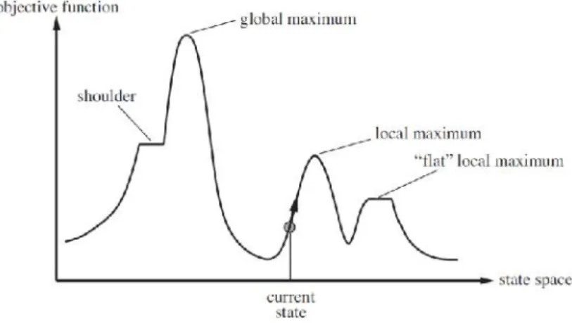
A hypothetical state space landscape is demonstrated in Figure 4-1 (Russell & Norvig, 2010). In the figure, current state represents the current best solution and elevation is value of the objective function. Objective function can aim to find the highest peak (global maximum) or lowest valley (global minimum). Local search algorithms aim to search through the solution space to find a local optimum value.

(55)

Figure 4-1 A one-dimensional state-space landscape in which elevation corresponds to the objective function (Russell & Norvig, 2010)

Some algorithms are greedy and this may cause them to become stuck in local minimum or maximum. A pure random move can be useful to avoid such circumstances, but this may be very expensive and sometimes it may not be useful. Various techniques to avoid being stuck in local hills and valleys are proposed. One of such techniques is used in the simulated annealing algorithm, which has been applied to many problems successfully. Annealing is the process of heating up metals to high temperatures, and then leaving them to cooling for a while and heating them up again. While increasing the temperature of the metal for a small period of time, the process allows metal to move in opposite direction. Stuart and Norvig (2010) gave a ball example to explain the simulated annealing approach. If a ball is thrown to the search space, ball will get stuck in the first local optimum. If ground (search space) is shaken, ball can move out of its current state and advance to the next valley. In most simulated annealing implementations, the size of the shake is bigger at the beginning of the search. The size of the shake decreases gradually as the algorithm runs.

4.1 NEH Algorithm

NEH (Nawaz, Enscore, & Ham, 1983) is the best known and most efficient heuristic for flowshop scheduling problem. NEH algorithm aims to insert new jobs into best position in the permutation of partially scheduled jobs. The best position is the position that results in minimum partial fitness function value. The worst-case

(56)

complexity of the algorithm is . In 1990, Taillard (Taillard, 1990) proposed a new calculation method for makespan calculation in flowshop problems that decreases the computational complexity of the algorithm from to . NEH algorithm became more efficient and popular in flowshop problems with this improvement for makespan minimization criterion.

Basic NEH algorithm consists of two stages. In the first stage, jobs are sorted according to their total processing times on all machines. In the second stage, the jobs are considered one by one in order for insertion into the partial schedule. The jobs are inserted in all possible positions in the partial schedule and the position that minimizes the partial fitness value is selected for insertion. The pseudo-code of the NEH algorithm is given in Figure 4-2.

Figure 4-2 Pseudocode of the NEH algorithm

(Taillard, 1990) constructs earliest completion times ( ) and tail ( ) matrices before executing Step 3.2 in order to calculate partial makespan values in one operation instead of using operations.

Adaptations and modifications to NEH algorithm has been proposed for different versions of the flowshop problem. For example, Rios-Mercado and Bard (Rios-Mercado & Bard , 1998b) extended the algorithm to consider sequence dependent setup times (SDST) in the calculation and named their algorithm as NEHT-RB (Nawaz-Enscore-Ham, Taillard, Rios-Mercado and Bard). and matrixes are calculated