A line based pose representation for human action recognition

(1)

A LINE BASED POSE REPRESENTATION

FOR HUMAN ACTION RECOGNITION

a thesis

submitted to the department of computer engineering

and the institute of engineering and science

of bilkent university

in partial fulfillment of the requirements

for the degree of

master of science

By

Sermetcan Baysal

January, 2011

(2)

I certify that I have read this thesis and that in my opinion it is fully adequate, in scope and in quality, as a thesis for the degree of Master of Science.

Asst. Prof. Dr. Pınar Duygulu(Advisor)

Asst. Prof. Dr. Selim Aksoy

Prof. Dr. Aydın Alatan

Approved for the Institute of Engineering and Science:

Prof. Dr. Levent Onural Director of the Institute

(3)

ABSTRACT

A LINE BASED POSE REPRESENTATION FOR

HUMAN ACTION RECOGNITION

Sermetcan Baysal M.S. in Computer Engineering Supervisor: Asst. Prof. Dr. Pınar Duygulu

January, 2011

In this thesis, we utilize a line based pose representation to recognize human ac-tions in videos. We represent the pose in each frame by employing a collection of line-pairs, so that limb and joint movements are better described and the geo-metrical relationships among the lines forming the human figure is captured. We contribute to the literature by proposing a new method that matches line-pairs of two poses to compute the similarity between them. Moreover, to encapsulate the global motion information of a pose sequence, we introduce line-flow histograms, which are extracted by matching line segments in consecutive frames. Experi-mental results on Weizmann and KTH datasets, emphasize the power of our pose representation; and show the effectiveness of using pose ordering and line-flow histograms together in grasping the nature of an action and distinguishing one from the others. Finally, we demonstrate the applicability of our approach to multi-camera systems on the IXMAS dataset.

Keywords: Human motion, action recognition, pose similarity, pose matching,

line-flow.

(4)

¨

OZET

˙INSAN HAREKETLER˙IN˙IN TANINMASI ˙IC¸˙IN C¸˙IZG˙I

TABANLI B˙IR POZ TEMS˙IL˙I

Sermetcan Baysal

Bilgisayar Mühendisli˘gi, Yüksek Lisans Tez Yöneticisi: Y. Doc. Dr. Pınar Duygulu

Ocak, 2011

Bu tezde videolardaki insan eylemlerini tanımak i¸cin ¸cizgiye dayalı bir poz tem-silinden faydalanılmaktadır. Her karedeki pozu ¸cizgi-¸ciftleri kullanarak tem-sil ediyoruz; böylece el, kol ve eklem hareketlerini daha iyi tanımlamı¸s, in-san figürünü olu¸sturan ¸cizgiler arasındaki geometrik ili¸skileri yakalamı¸s oluy-oruz. ˙Iki poz arasındaki ¸cizgi-¸ciftlerini e¸sle¸stirerek benzerliklerini hesaplayan yeni bir yöntem önererek literatüre katkıda bulunuyoruz. Dahası, poz dizilerindeki genel hareket bilgisinin saklanması i¸cin ardı¸sık karelerdeki ¸cizgileri e¸sle¸stirerek olu¸sturulan ¸cizgi-akı¸s histogramlarını sunuyoruz. Weizmann ve KTH veri set-leri üzerindeki deneysel sonu¸clar, poz temsilimizin gücünü vurgulamakta; be-raber kullanıldıklarında, sıralı poz ve ¸cizgi-akı¸s histogramlarının bir eylemin do˘gasını kavrayarak birini di˘gerlerinden ayırt edebilme üzerindeki etkinli˘gini göstermektedir. Son olarak, yakla¸sımımızın ¸coklu kamera sistemlerine uygulan-abilirli˘gini IXMAS veri seti üzerinde göstermekteyiz.

Anahtar s¨ozc¨ukler : ˙Insan hareketi, eylem tanıma, poz benzerli˘gi, poz e¸sleme, ¸cizgi-akı¸sı.

(5)

Acknowledgement

First and foremost, I owe my deepest gratitude to my supervisor, Dr. Pınar Duygulu, for her encouragement, guidance and support throughout my studies. She has been my inspiration as I hurdle all the obstacles in the completion of this thesis.

I am grateful to the members of my thesis committee, Asst. Prof. Dr. Selim Aksoy and Prof. Dr. Aydın Alatan for accepting to read and review my thesis and for their insightful comments.

I offer my regards and blessings to all my friends and office mates who sup-ported me in any aspect during my research. Especially, I am grateful to Mehmet Can Kurt for sharing his ideas and for the good partnership. I also would like to make a special reference to G¨ulden Yılmaz for her invaluable support.

Last but not the least, I would like to very much thank to my parents, ˙Inci and Ayhan Baysal for always being cheerful and supportive. None of this would have been possible without their love.

(6)

List of Figures

1.1 The overview of our approach . . . 5

3.1 Steps of pose extraction . . . 11

3.2 Steps of noise elimination . . . 12

3.3 Spatial binning of a human figure . . . 13

3.4 Matched line-pairs in similar poses . . . 15

3.5 Matched line-pairs in similar and slightly different poses . . . 16

3.6 Representing line-flow vectors . . . 17

3.7 Action recognition using only single pose information . . . 19

3.8 Alignment of two pose sequences . . . 21

3.9 Global line-flow of different actions . . . 22

4.1 Example frames from the Weizmann dataset . . . 25

4.2 Example frames from the KTH dataset . . . 26

4.3 Example frames from IXMAS dataset . . . 27

4.4 Recognition accuracies of different classification methods . . . 31

(10)

LIST OF FIGURES x

4.5 Confusion matrix of each classification method for the Weizmann dataset . . . 32

4.6 Confusion matrix of PO+LF classification method for the KTH dataset . . . 33

4.7 Recognition accuracies on different scenarios in the KTH dataset . 33

4.8 Recognition accuracy of PO+LF classification method with respect to α . . . . 35

4.9 Recognition accuracies of different cameras for each action in the IXMAS dataset . . . 36

(11)

List of Tables

4.1 Effect of using different pose similarity calculation functions and spatial-binning values . . . 29

4.2 Recognition accuracies on IXMAS dataset . . . 37

4.3 Comparison of our approach to other studies over the KTH dataset 38

4.4 Comparison of our results with respect to different features . . . . 39

4.5 Comparison of our approach to other studies over the IXMAS dataset 39

(12)

Chapter 1 Introduction

1.1 Motivation

Recognizing and analyzing human actions in videos has been receiving increas-ing attention of computer vision researchers both from academia and industry. A reliable and an effective solution to this problem is essential for a large vari-ety of applications. For instance, tracking the human body throughout a video is particularly useful for athletic performance analysis and medical diagnostics; building a visual surveillance system that monitors human actions in security-sensitive areas such as streets, airports and borders will aid police and military forces [1]. Moreover, recognizing simple human actions in real-time is a neces-sity for building more sophisticated human-computer interactions systems such as game console which does not require any type of gamepad.

Motivated by the fact that a robust system can provide great benefits to a variety of application areas, this thesis tries to address the problem of automat-ically recognizing human actions1 _{in videos. However, finding a solution to this}

problem is challenging since people can perform the same action in unique ways with various execution speeds. Furthermore, recording conditions may differ as

1_{As in [36], by ‘actions’ we refer to simple motion patterns executed by a single person that}

last for short period of time. (e.g. bending, kicking, punching, walking, waving, etc.).

(13)

CHAPTER 1. INTRODUCTION 2

well. Videos could be recorded under different illumination conditions, at differ-ent scales and from differdiffer-ent viewpoints. In order to build an action recognition system that can handle these challenges, representation of an action is crucial.

The human brain can more or less recognize what a person is doing in a video even by looking at a single frame without examining the whole sequence. From this observation it can be deduced that the human pose encapsulates useful in-formation about the action being performed. Therefore, we use human pose as our primitive action units in our study. Since a single pose only provides instan-taneous information, which may be in common with other actions, we employ a sequence of poses to incorporate temporal information in the simplest way.

Some of the previous studies [4, 5, 28] attempt to represent the shape of a pose by using background subtracted human silhouettes. Although these approaches are robust to variations in the appearance of actors, they require static cameras and a good background model, which may not be possible under realistic con-ditions [15]. A more severe limitation of such methods is that they ignore limb movements remaining inside the silhouette boundaries; as a results, ‘standing still’ is likely to be confused with ‘hand clapping’ when the action is performed facing the camera and hands are in front of the torso.

An alternative shape representation can be established using contour features. Motivated by the work of Ferrari et al. in [10], where encouraging results were obtained using line segments as descriptors for object recognition, we represent the shape of a pose as a collection of line segments fitted to the contours of a human figure. We believe that such a representation is more applicable to realistic conditions compared to silhouette-based methods.

Utilizing only shape information may fail to capture differences between ac-tions with similar pose appearances, such as ‘running’ and ‘jogging’. In such cases the speed and direction of the movement in different parts of the body is important in making a discrimination. When identifying differences between those actions with similar appearances, global motion cues can be helpful. There-fore, in addition to our pose-based action representation, we also extract global line-flow histograms for a pose sequence by matching lines in consecutive frames.

(14)

1.2 Overview and Contributions

This section presents the overview of our approach (depicted in Figure 1.1) and highlights our contributions.

For each frame, contour information is extracted using the high-performance contour detector (GPB) presented in [24]. Then a Contour Segment Network (CSN) consisting of roughly straight lines is constructed. Next, the human figure is detected by utilizing the densest area of line segments.

In order to capture geometrical relationships among the lines forming the human figure, the pose in each frame is represented by a collection of line-pairs. The similarity between two poses are measured by matching their line-pairs and the pose ordering of two sequences are compared using Dynamic Time Warping (DTW). To obtain the global line-flow of a pose sequence, line displacement vectors are extracted for each frame by matching its set of lines with the ones in the previous frame. Then these vectors are represented by a single compact line-flow histogram.

Given a sequence of poses, recognition is performed by employing separate weighted k -nearest neighbor (k -NN) classifiers for both pose ordering and global line-flow. Then their decisions are combined using a simple linear weighted scheme in order to obtain the final classification.

In this work, we mainly concentrate on the representation of actions and make two contributions to the literature. Firstly, we propose a new matching method2 between two poses to compute their similarity. Secondly, we introduce global line-flow to encapsulate motion information for a collection of poses formed by line segments.

2_{A preliminary version of this matching method was presented in [3] at International}

(15)

1.3 Organization of the Thesis

The remainder of this thesis is organized as follows.

Chapter 2 presents a review of recent studies on action recognition and pro-vides a discussion of related studies.

Chapter 3 describes our approach to recognize human actions. It gives de-tails of our pose representation, proposed pose matching method and line-flow extraction.

Chapter 4 evaluates the performance of our approach on the state-of-art action recognition datasets and compares our results to the previous studies.

Chapter 5 concludes the thesis giving a summary and discussion of our ap-proach and describes possible future work.

(16)

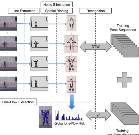
Figure 1.1: The overview of our approach (best viewed in color). Step 1: Line

Extraction. For each frame, a Contour Segment Network (CSN) consisting of

roughly straight lines is constructed. Step 2: Noise Elimination and

Spa-tial Binning. The human figure is detected by utilizing the densest area of line

segments. Then a N × N grid structure is placed over the human figure for lo-calization of the segments. Step 3: Line-Flow Extraction. Line displacement vectors are extracted for each frame by matching its set of lines with the ones in the previous frame. Then these vectors are represented by a single compact line-flow histogram. Step 4: Recognition. The ordering of poses and global line-flow histogram of test sequences are compared to the stored templates us-ing DTW and χ2 distance respectively. Recognition is performed by employing separate weighted k -NN classifiers and combining their decisions for both pose ordering and global line-flow.

(17)

Chapter 2 Related Work

Human action recognition has been a widely studied topic of computer vision. Many approaches have been proposed which use different ways to represent ac-tions and extract features. In this chapter, we will give a brief review and discus-sion of these studies.

2.1 Review of Previous Studies

2.1.1 Utilizing Space-Time Volumes

The following group of studies utilize space-time volumes. Blank et al. [4] regard human actions as 3D shapes induced by the silhouettes in the space-time volume. Similarly, Ke et al. [15] segment videos into space-time volumes, however their spatio-temporal shape based correlation algorithm does not require background subtraction. In another study [28], Qu et al. employ 2D silhouettes in the space-time volume as a basis for useful feature extraction and propose a global feature that extracts the difference points between images.

(18)

CHAPTER 2. RELATED WORK 7

2.1.2 Employing Space-Time Interest Points

There are a large number studies which employ space-time interest points (STIP) for action representation. Dollar et al. [7] propose a spatio-temporal interest point detector based on 1D Gabor filters to find local regions of interest in space and time (cuboids) and use histograms of these cuboids to perform action recognition. These linear filters were also applied in [20, 25, 26] to extract STIP. In addition to the utilization of cuboids, Liu et al. [21] employ higher-order statistical model of interest points, which aims to capture the global information of the actor. There are also other studies which use different spatio-temporal interest point detectors. Laptev et al. [17] detect interest points using a space-time extension of the Harris operator. However, instead of performing a scale selection, multiple levels of spatio-temporal scales are extracted. The same STIP detection technique is also adopted by Thi et al. in [34]. They extend Implicit Shape Model to 3D, enabling them to robustly integrate the set of local features into a global configuration, while still being able to capture local saliency.

Among the STIP based approaches, [7, 17, 19, 25] quantize local space-time features to form a visual vocabulary and construct a bag-of-words model to rep-resent a video. However, Kovashka et al. and Ta et al. believe that the orderless bag-of-words lacks cues about motion trajectories, before-after relationships and spatio-temporal layout of the local features which may be almost as important as the features themselves. So, Kovashka et al. [16] propose to learn shapes of space-time feature neighbors that are most discriminative for an action category. Similarly, Ta et al. [33] present pairwise features (STIP are connected if they are close both in space and time), which encode both the appearance and the spatio-temporal relations of the local features for action recognition.

2.1.3 Flow-Based

This group of studies use flow-based techniques which estimate the optical field between adjacent frames to represent of actions. In [8], Efros et al. introduce

(19)

a motion descriptor based on blurred optical flow measurements in a spatio-temporal volume for each stabilized human figure, which describes motion over a local period of time. Wang et al. [37] also use the same motion descriptor for frame representation and represent video sequences by a bag of words rep-resentation. Fathi et al. [9] extends the work of Efros to a 3D spatio-temporal volume. They propose a method constructing mid-level motion features which are build from low-level optical flow information. Different from the flow-based studies above, Ahmad et al. [2] represent action as a set of multi-dimensional combined local-global (CLG) optic flow and shape flow feature vectors in the spatio-temporal action boundary.

2.1.4 Shape-Based

Actions are represented by poses in the following studies. Carlsson et al. [6] demonstrate that specific actions can be recognized by matching shape infor-mation extracted from individual frames to stored prototypes representing key frames of an action. Following this study and using the same shape matching scheme, which compares edge maps of poses, Loy et al. [22] present a method for automatically extracting key frames from an image sequence. Ikizler et al. [14] propose a bag-of-rectangles method that represents human body as a collection of rectangular patches and calculate their histograms based on their orientation. Hatun et al. [12] describe pose in each frame using the histogram of gradients (HOG) features obtained from radial partitioning of the frame. Similarly, Thurau et al. [35] extend HOG based descriptor to represent pose primitives. In order to include local temporal context, they compute histograms of n-gram instances.

2.1.5 Combining Shape and Motion

The final group of studies combine both shape (pose) and motion (flow) features to represent actions. In a closely related study, Ikizler et al.[13] introduce a new shape descriptor based on the distribution of lines fitted to the boundaries of human figures. Poses are represented by employing histogram of lines based

(20)

on their orientations and spatial locations. Moreover, a dense representation of optical flow and global temporal information is utilized for action recognition. Schindler et al. [31] propose a method that separately extracts local shape, using the responses of Gabor filters at multiple orientations, and dense optic flow from each frame. Then the shape and flow feature vectors are merged by simple concatenation before applying SVM classification for action recognition. Lin et al. [18] capture correlations between shape and motion cues by learning action prototype trees in a joint features space. The shape descriptor is formed by simply counting the number of foreground pixels either in silhouettes or appearance-based likelihoods. Their motion descriptor is an extension of the one introduced by Efros et al. [8], in which background motion components are removed.

2.2 Discussion of Related Studies

Studies of Hatun et al. [12], Ikizler et al.[13, 14] and Thurau et al. [35], share a common property of employing histograms to represent the pose information in each frame. However, using histograms for pose representation results in the loss of geometrical information among the components (e.g. lines, rectangles, gradients) forming the pose. For action recognition such a loss is intolerable since configuration of the components is very crucial in describing the nature of a human action involving limb and joint movements. Representing the pose in a frame as a collection of line-pairs, our work differs from these studies by preserving the geometrical configuration of components encapsulated in poses.

In this study, we propose to capture the global motion information in a video by tracking line displacements across adjacent frames, which could be compared to optical flow representations in [2, 8, 9, 37]. Although, optical flow often serves as a good approximation of the true physical motion projected onto the image plane; in practice, its computation is susceptible to noise and illumination changes as stated in [36]. Lines are less effected by variations in the appearance of actors and they are easier to track than lower-level features such as color/intensity changes. Thus, we believe that line-flow could be a good alternative to optical flow.

(21)

Chapter 3 Our Approach

In this chapter we present our approach to recognize human actions. First, we give the details of our line-based pose extraction (Section 3.1) and then our proposed pose matching method is presented (Section 3.2). Next, we describe the derivation of line-flow histograms (Section 3.3). Having explained our feature extraction steps in previous sections, finally, we describe the action recognition phase of our approach (Section 3.4).

3.1 Line-Based Pose Extraction

Pose in each frame is extracted as follows (depicted in Figure 3.1):

1. The global probability of boundaries (GPB), which is presented by Maire et al. as a high-performance detector for contours in natural images (see [24] for details), are computed to extract the edges of the human figure in a frame.

2. To eliminate the effect of noise caused by short and/or weak edges, hys-teresis thresholding is applied to obtain a binary image consisting of edge pixels (edgels).

(22)

CHAPTER 3. OUR APPROACH 11

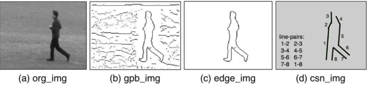
Figure 3.1: This figure illustrates the steps of pose extraction. Given any frame (a), GPB are computed to extract the contours (b). Then hysteresis thresholding is applied to obtain a binary image consisting of edge-pixels (edgels) (c). Next, edgel-chains are partitioned into roughly straight contour segments forming the CSN (d). Finally, CSN is represented by k AS descriptor.

3. Edgels are chained by using closeness and orientation information. The edgel-chains are partitioned into roughly straight contour segments. This chained structure is used to construct a contour segment network (CSN). 4. The CSN is represented by scale invariant k -Adjacent Segment (k AS)

de-scriptor encoding the geometric configuration of the segments, which was introduced by Ferrari et al. in [10].

As defined in [10], the segments in a k AS form a path of length k through the CSN. Two segments are considered as connected in the CSN, when they are adjacent along some object contour even if there is a small gap separating them physically. More complex structures can be captured as k increases in a k AS. 1AS are just individual lines, 2AS include L-shapes and 3AS can form C, F and Z shapes.

Human pose, especially limb and joint movements, can be better described by using L-shapes. Therefore, in our work we select k =2, and refer to 2AS features as line-pairs. Example line-pairs can be seen in Figure 3.1 (d). Each line-pair consisting of line segments s1 and s2 is represented with the following descriptor:

Vline−pair = ( rx 2 Nd , r y 2 Nd , θ1, θ2, l1 Nd , l2 Nd ) (3.1)

(23)

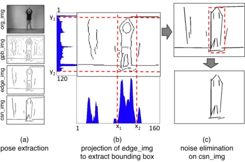
Figure 3.2: This figure illustrates the steps of noise elimination. Notice that after the pose extraction steps, the CSN contains erroneous line segments that do not belong to the human figure (a). So in (b), edge img is projected onto x and y axes to form a bounding box around the densest area of line segments in the

csn img. Line segments that remain outside the bounding box are eliminated

form the CSN (c).

where r2 = (rx2, r y

2) is the vector going from midpoint of s1 to midpoint of s2, θi

is the orientation and li = ∥si∥ is the length of si (i = 1, 2). Nd is the distance

between the two midpoints, which is used as the normalization factor.

3.1.1 Noise Elimination

Under realistic conditions (varying illumination, cluttered backgrounds, reflection of shadows, etc.) the edge detection results may contain erroneous line segments that do not belong to the human figure. So, assuming that the densest area of line segments in the CSN contains the human figure, the following noise elimination steps are applied after pose extraction (depicted in Figure 3.2):

1. Project edge img onto the x-axis. Then for each isolated curve, calculate its integral with respect to the x-axis. Set x1 and x2 to be the boundaries

(24)

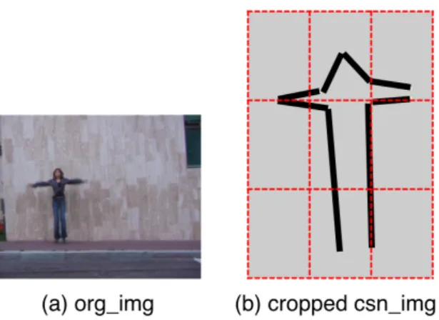
Figure 3.3: This figure illustrates the spatial binning applied to a human pose. The original frame can be seen in (a). After detecting the human figure in the

csn img, by the means of a bounding box, the frame is then divided into

equal-sized spatial bins so that an N × N grid structure is formed. In (b) an example of spatial binning is illustrated for N =3.

2. Project edge img onto the y-axis. Then for each isolated curve, calculate its projected length on the y-axis. Set y1 and y2 to be the boundaries of

the longest curve.

3. Place a bounding box on the csn img with (x1, y1) and (x2, y2) being its

upper left and lower right corner coordinates respectively.

4. Recall that the csn img contains a set of line segments such that csn img = {l1, l2, . . . , ln}. Eliminate a line segment li ∈ csn img from the CSN, if

its center’s coordinates is not in the bounding box.

3.1.2 Spatial Binning

The descriptor presented in [10] (Equation 3.1), encodes scale, orientation and length of the line-pairs, but it lacks position information. Therefore, in order to capture spatial locations of the line-pairs; first, the human figure is cropped from the frame using the bounding box which was previously formed in the noise elimination process. Then, to be used in the latter stages, the human figure is divided into equal-sized spatial bins forming an N × N grid structure. This process is depicted in Figure 3.3.

(25)

3.2 Finding Similarity Between Poses

Recall that pose in each frame is represented by a set of line-pair descriptors. The similarity between two line-pair descriptors va and vb is computed by the

following formula as suggested in [10]:

dline−pair(a, b) = wr· ∥r2a− r b 2∥ + wθ· 2 ∑ i=1 Dθ(θai, θ b i) + 2 ∑ i=1 log(la_i/lb_i) (3.2) where the first term is the difference in the relative location of the line-pairs, the second term measures the orientation difference of the line-pairs and the last term accounts for the difference in lengths. The weights of the terms are wr = 4

and wθ = 2. Note that Equation 3.2, proposed in [10], computes the similarity

only between two individual line-pairs. However, we need to compare two poses. Therefore, in this thesis, we introduce a method to find similarity between two frames consisting of multiple line-pairs.

3.2.1 Pose Matching

To compute a similarity value between two frames, first of all, we need to find a correspondence between their line-pairs. Any two frames consisting of multiple line-pair descriptors can mathematically be thought of as two sets X and Y with different cardinalities. We seek for a ‘one-to-one’ match between two sets so that an element in X is associated with exactly one element in Y . For instance, xi and

yj are matched if and only if g(xi) = yj and h(yj) = xi where g : X → Y, h :

Y → X, xi ∈ X, yj ∈ Y .

To describe our pose matching mechanism more formally, let f1 and f2 be

two frames having a set of line-pair descriptors Φ1 = {v11, v12, . . . , vn1} and Φ2 =

{v2

1, v22, . . . , vm2}, where n and m are the number of line-pair descriptors in Φ1

and Φ2 respectively. We compare each line-pair descriptor vi1 ∈ Φ1 with each

line-pair descriptor v2

(26)

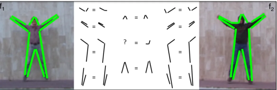
Figure 3.4: This figure illustrates the matched line-pairs in two frames having similar poses.

if and only if among descriptors in Φ2, v2j has the minimum distance to v1i and

among descriptors in Φ1, vi1 has the minimum distance to vj2. To include location

information, we apply a constraint in which matching is allowed only between line-pairs within the same spatial bin.

As an output of our pose matching method two matrices, D and M of size

n×m, are generated. D stores similarity of each line-pair in f1to each line-pair in

f2, where D(i, j) indicates the similarity value between vi1 and v2j. M is a binary

matrix, where M (i, j) = 1 indicates that i-th line-pair in f1 and j-th line-pair in

f2 are matched. These matrices are utilized when an overall similarity distance

between two frames is calculated.

3.2.2 Calculating a Similarity Value

Having established a correspondence between frames f1 and f2 by matching their

line-pairs, now we need to numerically express this correspondence. The first approach would be to take the average of the matched line-pair distances. This could be calculated by utilizing the matrices D and M as follows:

sim1(f1, f2) =

sum(D∧ M) |match(f1, f2)|

(3.3)

(27)

Figure 3.5: This figure (best viewed in color) illustrates matched line-pairs in sim-ilar (a) and slightly different (b) poses. Red lines (straight) denote the matched line-pairs common in both (a) and (b). Blue lines (dashed) indicate that these line-pairs are only matched in (a). sim1(f1, f2) is calculated by taking the

aver-age of red and blue lines (assuming that they represent a distance value between matching line-pairs) and sim1(f2, f3) is calculated by averaging only the red lines.

Since red lines are common in both scenarios, similarity distance in (a) may be very close to or even greater than (b) depending on the distances represented by blue lines. Therefore, unmatched line-pairs, shown by blue dots in (b), should be utilized to produce a ‘stronger’ similarity distance.

|match(f1, f2)| is the number of matched line-pairs between f1 and f2.

The function sim1, calculates a ‘weak’ similarity value between f1 and f2,

since it utilizes distances between only the matched line-pairs. However, poses of distinct actions may be very similar, differing only in configuration of a single limb (see Figure 3.5). To compute a ‘stronger’ similarity value, unmatched line-pairs in both f1 and f2 should be utilized. Thus, we present another similarity

value calculation function sim2, which assumes that a perfect match between sets

X and Y is established when both sets have the equal number of elements and

both ‘one-to-one’ and ‘onto’ set properties are satisfied, so that each element in

X is exactly associated with one element in Y . The function sim2 calculates the

overall similarity distance by penalizing unmatched line-pairs in the frame having more number elements as follows:

sim2(f1, f2) =

sum(D∧ M) + p · (max(m, n) − |match(f1, f2)|)

(28)

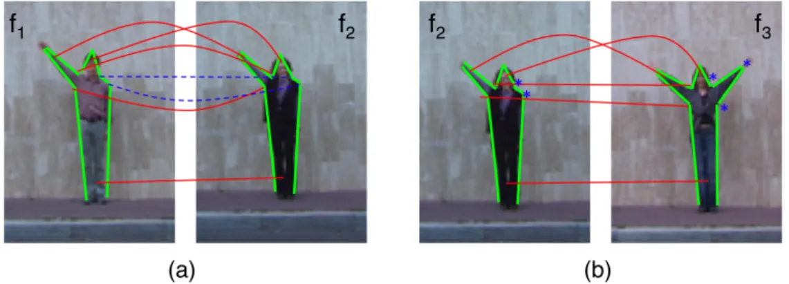
Figure 3.6: This figure illustrates extraction of line-flow vectors and histograms for a single frame (best viewed in color). Given an action sequence, i-th frame is matched with the previous (i−1)-th frame. Line-flow vectors (in green) show the displacement of matched lines with respect to the previous frame. Each line-flow vector is then separated into 4 non-negative components. We employ a histogram for each spatial bin to represent these line-flow vectors.

where p = mean(D∧ ¬M) is the penalty value, which denotes the average dis-similarity between two frames. The penalty is computed by excluding matched line-pair values and taking average of the remaining distances between all the other unmatched line-pairs. Relative performance of sim1 and sim2 will be

eval-uated in Chapter 4.

3.3 Line-Flow Extraction

By utilizing only shape information, it is sometimes difficult to distinguish actions having similar poses. In such cases, the speed of transition from a pose to the next one is crucial in distinguishing actions. In our work, we characterize this transition by extracting global flow of lines throughout an action sequence.

Given an action sequence, consecutive frames are compared to find matching lines. The same pose matching method in Section 3.2.1 is applied, however this time lines are matched instead of line-pairs. To do so, Equation 3.2 is modified

(29)

as follows to compute a distance between two line segments :

dline(a, b) = wθ· Dθ(θa, θb) +log(la/lb) (3.5)

where the first term is the the orientation difference of the lines and the second term accounts for the difference in lengths. The weighting coefficient is wθ = 2.

As depicted in Figure 3.6, after finding matches between consecutive frames, the displacement of each matched line with respect to the previous frame is represented by a line-flow vector ⃗F . Then this vector is separated into 4

non-negative components ⃗F = {F_x+, F_x−, F_y+, F_y−}, representing its magnitudes when

projected on x+, x−, y+ and y− axes on the xy-plane. For each j-th spatial bin, where j ∈ {1, . . . , N × N}, we define line-flow histogram hj(i) as follows:

hj(i) =

∑

k∈Bj

⃗

Fk (3.6)

where ⃗Fk represent a line-flow vector in spatial bin j. Bj is the set of flow vectors

in spatial bin j and i ∈ {1, . . . , n}, where n is the number of frames in the action sequence. To obtain a single line-flow histogram h(i) for the i-th frame, we concatenate line-flow histogram hj of each spatial bin j.

3.4 Recognizing Actions

Given the details of our feature extraction steps in the previous sections, we now the describe our action recognition methods in the following subsections.

3.4.1 Using Single Pose Information

This classification method explores the idea of using only single pose information for action recognition. In addition, it is used to evaluate our pose matching

(30)

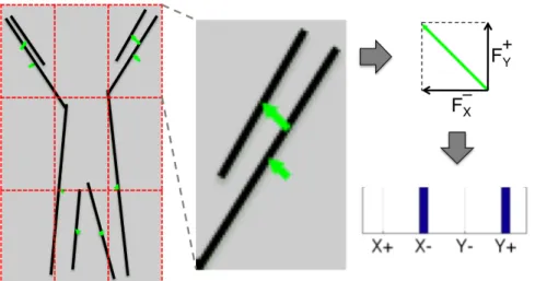
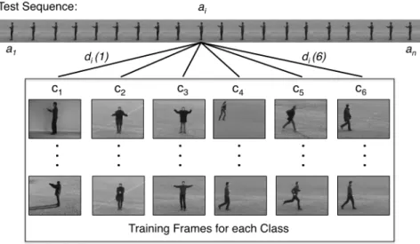
Figure 3.7: This figure illustrates the classification of an action sequence utilizing only single pose information throughout the video. For each frame in the test sequence, its distance to each class is computed by finding the most similar train-ing frame from that class. In order to classify the sequence, we take the average distance of all frames to each class and assign the class label with the smallest average distance.

mechanism, since it discards the order of poses and performs classification based on individual votes of each frame. Therefore, the performance of this method directly depends on the accuracy of our pose matching.

Given a sequence of images A = {a1, a2, . . . , an} to be classified as one of the

available classes C = {c1, c2, . . . , cm}, we calculate the similarity distance di(j)

of each frame ai ∈ A to each class cj ∈ C, by finding the most similar training

frame from class cj (depicted in Figure 3.7). In order to classify A, we seek for

the class having smallest average distance, where the average distance to each class cj ∈ C is computed as follows:

D(j) = n ∑ i=1 di(j) n (3.7)

(31)

3.4.2 Using Pose Ordering

Recognizing human actions by comparing individual poses as in Section 3.4.1 is likely to fail in distinguishing actions such as ‘sitting down’ and ‘standing up’, which consist of the same set of poses in reverse order. Therefore, relative ordering of the poses should be utilized to construct a more accurate classification method.

In this classification method, recognition is performed by comparing two ac-tion sequences and finding a correspondence between their pose orderings. How-ever, comparing two pose sequences is not straightforward since actions can be performed with various speeds and periods, resulting in sequences with differ-ent lengths. Therefore, first we align two sequences by means of Dynamic Time Warping (DTW) [29] and then utilize the distance between aligned poses to derive an overall similarity.

DTW is an algorithm to compare time series and find the optimal alignment between them by means of dynamic programming. As formalized in [30], given two action sequences A = a1, a2, . . . , ai, . . . , a|A| and B = b1, b2, . . . , bj, . . . , b|B| of

lengths|A| and |B|, DTW constructs a warp path W = w1, w2, . . . , wK (depicted

in Figure 3.8) where K is the length of the warp path and wk = (i, j) is the

k-th element of warp path indicating that the i-th element of A and the j-th

element of B are aligned. Using the aligned poses, the distance between two action sequences A and B is calculated as follows:

DistDT W(A, B) = K ∑ k=1 dist(wki, wkj) K (3.8)

where dist(wki, wkj) is the distance between two frames ai ∈ A and bj ∈ B, which

are aligned at the k-th index of the warp path, calculated using our pose matching function. Refer to [30] for the details of finding the minimum-distance warp path using a dynamic programming approach.

(32)

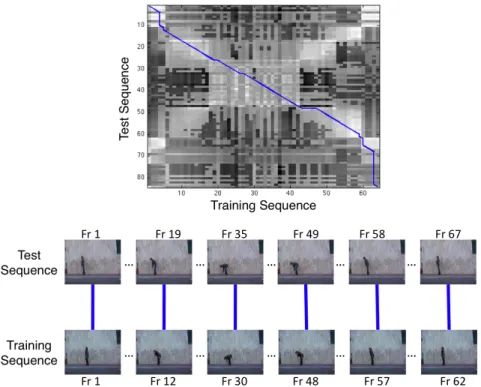
Figure 3.8: This figure illustrates the alignment of two action sequences. Frame-to-frame similarity matrix of two actions can be seen on the top. Brighter pixels indicate smaller similarity distances (more similar frames). The ‘blue line’ overlaid on the matrix indicates the warp path obtained by DTW. The frame correspondence based on the alignment path is shown on the bottom.

to the class most common amongst its k nearest training pose sequences using

DistDT W (Equation 3.8) as its distance metric. In addition we weight the

contri-butions of the neighbors by 1/d, where d is the distance to the test sequence, so that nearer neighbors contribute to the decision more than the distant ones. We denote this classifier as cpose to be used in Section 3.4.4.

3.4.3 Using Global Line-Flow Histograms

In Section 3.3, the extraction of a line-flow histogram h(i) for a single frame was shown. In order to represent a video, we simply sum up line-flow histograms of each frame to from a single compact representation of the entire action sequence consisting of n frames as follows:

(33)

Figure 3.9: This figure illustrates the global line-flow of different actions (from

left to the right): bend, jumping jack, jump in place, running and walking.

Notice that the line-flow vectors are in different orientations in different spatial locations so that ‘bend’, ‘jumping jack’ and ‘jump in place’ can be easily distin-guished. Although, the global line-flow of ‘running’ and ‘walking’ seem similar, notice the difference in the density of the lines. Sparser lines represent faster motion, whereas dense lines represent actions with slower motion.

H =

n

∑

i=1

h(i) (3.9)

We compute the flow similarity between two action sequences A and B by comparing their global line-flow histograms Ha and Hb using chi-square distance

χ2 as follows: χ2(A, B) = 1 2 ∑ n (Ha(n)− Hb(n))2 Ha(n) + Hb(n) (3.10)

In order to classify a given pose sequence, we employ a weighted k -NN classifier (as in Section 3.4.2) which uses χ2 _{(Equation 3.10) as its distance metric. This}

classifier is denoted as cf low to be used in Section 3.4.4. The global line-flow of

different actions can be seen in Figure 3.9.

3.4.4 Using Combination of Pose Ordering and Line-Flow

In the previous sections, two action recognition methods were introduced. The first one utilizes pose ordering of an action sequence and the second one captures the global motion cues by using line-flow histograms. These two methods are

(34)

combined in this final classification scheme, in order to overcome limitations of either shape or flow-based behaviors and achieve a higher accuracy.

To classify a given pose sequence, we employ decision vectors ⃗dpose and ⃗df low,

generated by the weighted k -NN classifiers cpose (see Section 3.4.2) and cf low (see

Section 3.4.3) respectively. Each decision vector is normalized such as ⃗d(i)∈ [0, 1]

for all i∈ {1, 2, . . . , n}, where ⃗d(i) is the probability of the test sequence belonging to the i-th class and n is the number of classes. We combine the two normalized decision vectors ⃗dpose and ⃗df low using a simple linear weighting scheme to obtain

the final decision vector ⃗dcombined as follows:

⃗

dcombined = α· ⃗dpose+ (1− α) · ⃗df low (3.11)

where α is the weighting coefficient of the decision vectors. It determines the relative influence of pose (shape) and line-flow (motion) features on the final classification. Finally, the test pose sequence is assigned to the class having the highest probability value in the combined decision vector ⃗dcombined. The effect of

(35)

Chapter 4 Experiments

In this chapter we evaluate the performance of our approach. First we introduce the state-of-art action recognition datasets (Section 4.1). Then we give details of our experiments and results (Section 4.2). Finally, we compare our results to the related studies and provide a discussion (Section 4.3)

4.1 Datasets

In our experiments, we evaluate our method on the Weizmann and the KTH datasets, which are currently considered as the benchmark datasets for single-view action recognition. In addition, further experiments are performed on the IXMAS multi-view dataset to show that our approach is applicable to multiple camera systems. We adopt leave-one-out cross validation as our experimental setup on all the datasets in order to compare our performance fairly and completely with other studies as recommended in [11].

(36)

CHAPTER 4. EXPERIMENTS 25

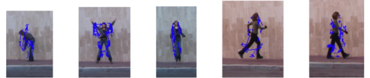
Figure 4.1: Example frames from the Weizmann Dataset [4] are shown for 9 different actions: top row from left to the right: bend, jumping jack, jump forward (jump); middle row from left to the right: jump in place (pjump), run, gallop sideways (side); bottom row from left to the right: walk, one-hand wave (wave1), two-one-hands wave (wave2).

4.1.1 Weizmann Dataset

This single-view dataset was introduced by Blank et al. in [4] containing 10 actions performed by 9 different actors. We use the same set of 9 actions for our experiments as in [4]; which are bend, jumping jack, jump forward, jump in place, run, gallop sideways, walk, one-hand wave and two-hands wave. Example frames are shown in Figure 4.1. For this dataset we used the available silhouettes, which were obtained using background subtraction, and applied canny edge detection to extract edges. So we start our pose extraction process (see Section 3.1) from step 3.

4.1.2 KTH Dataset

This dataset was introduced by Schuldt et al. in [32]. It contains 6 actions: box-ing, hand clappbox-ing, hand wavbox-ing, joggbox-ing, running and walking. Each action is

(37)

Figure 4.2: Example frames from KTH Dataset [32] are shown for 6 different actions on each row from top to the bottom: boxing, hand clapping, hand waving, jogging, running, walking. Frames on each column from left to the

right belong to one of 4 different shooting conditions: sc1, sc2, sc3 and sc4

performed by 25 subjects in 4 different shooting conditions: outdoor recordings with a stable camera (sc1), outdoor recordings with camera zoom effects and different viewpoints (sc2), outdoor recordings in which the actors wear different outfits and carry items (sc3), indoor recordings with illumination changes and shadow effects (sc4). Example frames are shown in Figure 4.2. KTH is consid-ered as a more challenging dataset compared to Weizmann due to its different realistic shooting conditions. In addition, it contains two similar actions: jogging and running. In this dataset, the length of a video generally exceeds 100 frames and actions are performed multiple times in a video. In order to reduce exten-sive computational cost, we trim the action sequences to 20-50 frames for our experiments so that an action in a video is performed only once or twice.

(38)

Figure 4.3: Example frames from IXMAS Dataset [39] are shown for various actions recorded using cameras with different viewpoints (on each column from

left to the right): cam1, cam2, cam3 and cam4

4.1.3 IXMAS Dataset

This dataset was introduced by Weinland et al. in [39]. It is a benchmark multi-view dataset in which 5 synchronized and calibrated cameras (cam1, cam2,

cam3, cam4, cam5) are used for recording. There are 13 actions: check watch,

cross arms, scratch head, sit down, get up, turn around, walk, wave, punch, kick, point, pick up and throw. Each action is performed three times (we only use the first of three performances of an actor for each action) with free orientation by 12 different actors. Example frames are shown in Figure 4.3. In our experiments, we omit the last camera (cam5), in which actors are shot from bird’s eye view, and use the remaining four cameras. For this dataset we used the available sil-houettes, which were extracted using background subtraction, and applied canny edge detection to extract edges. So we start our pose extraction process (see section 3.1) from step 3.

(39)

4.2 Experimental Results

In this section, we present the experimental results evaluating our approach in recognizing human actions. First, the effect of applying spatial binning is ex-amined (Section 4.2.1). Then, the optimal configuration of our pose similarity calculation function is founded (Section 4.2.2). Next, pose and flow features are evaluated (Section 4.2.3); and the effect of applying noise elimination is discussed (Section 4.2.4). Afterwards, regarding classification, the weighting between pose ordering and line-flow is examined. Finally, the applicability of our method to multi-camera systems is tested (Section 4.2.6).

4.2.1 Evaluation of Spatial Binning

Recall that in Section 3.1.2, we place an N× N imaginary grid structure over the human figure in order to capture the locations of line segments in a frame. The choice of N is important, because in our pose matching method we only allow matching between pairs within the same spatial bin. Similarly, during line-flow extraction between consecutive frames, lines are required to be in the same spatial bin in order to be matched. More importantly, since a line-flow histogram is extracted for each spatial bin, the choice of N directly effects the size of the global line-flow feature vector.

Table 4.1 compares the use of different-sized grid structures. The worst results are obtained when N = 1, which means that no spatial binning is used and matching is allowed between lines or line-pairs located anywhere in the frame.

N = 2 gives better results compared to no spatial binning and the best results

are obtained when a 3× 3 grid structure is placed over the human figure. This justifies that the spatial locations of the line-pairs provide useful clues when comparing poses. Regarding line-flow, we can infer from the results that using spatial binning and histogramming line-flow in each spatial bin better describes the local motion of separate body parts.

(40)

Table 4.1: Action recognition accuracies on Weizmann and KTH datasets using different classification methods (SP: Single Pose, PO: Pose Ordering, LF: Line-Flow) with respect to choice of pose similarity calculation functions (sim1 and

sim2) and different spatial binnings (N× N).

Weizmann KTH N = 1 N = 2 N = 3 N = 1 N = 2 N = 3 SP sim1 64.2% 71.6% 74.1% 61.7% 63.3% 66.3% sim2 92.6% 92.6% 93.8% 71.3% 75.0% 75.3% PO sim1 69.1% 81.5% 85.2% 74.3% 77.2% 81.3% sim2 92.6% 92.6% 95.1% 56.2% 68.5% 73.3% LF 48.1% 64.2% 87.7% 71.3% 74.8% 80.5%

4.2.2 Configuring Pose Similarity Calculation Function

After finding a correspondence between two poses by matching their line-pairs, in order to calculate an overall similarity between the frames, two pose similarity calculation functions were introduced in Section 3.2.1. Recall that sim1 utilizes

only the distances between matching line-pairs, whereas sim2 also penalizes the

unmatched line-pairs. Table 4.1 compares the relative performances of these functions. Observing the results, we deduce the following:

• When single pose based classification method is used, sim2 performs better

on both of the datasets. Since ordering of the poses is totally discarded in this classification method, the performance mainly depends on the accuracy of the similarity calculation function. A higher accuracy is obtained by

sim2 because of its strict constraints on pose matching which results in a

‘stronger’ function. More importantly, when comparing test poses to the stored templates, there is always a frame obeying these strict constraints, since the single pose based classification seeks for a matching pose within the set of all training frames (recall Figure 3.7).

• When pose ordering classification is used, notice that the accuracy of sim1

significantly increases for both of the datasets; whereas sim2 is about the

same for Weizmann, but decreases so that its below sim1 for KTH dataset.

(41)

including the ordering of poses in action recognition. Regarding the perfor-mance of sim2, we can say that since the data is ‘clean’ in the Weizmann

dataset, similar pose sequences can still be found under strict matching constraints, which slightly increases the accuracy. However, the accuracy of sim2 drops below sim1 for the KTH dataset. This means that requiring

strict matching constraints when comparing two poses in a ‘noisy’ dataset, results in addition of unrealistic penalty due to the high number of un-matched line-pairs that actually do not even belong to the human figure.

• In summary, sim2 is more accurate when the edges of the human figure are

successfully extracted and at classifying individual poses when pose order-ing is not available. However, it is wiser to employ sim1 in more realistic

data. Hence, sim2 function is used in the Weizmann and IXMAS datasets

where the edges are extracted from background subtracted silhouettes; sim1

is used in the KTH dataset where edges are extracted from contour infor-mation.

4.2.3 Evaluation of Pose and Flow Features

Having decided on the optimal spatial binning value and chosen a suitable pose similarity calculation function depending on the conditions, in this section, we evaluate the performance of pose and flow features in recognizing human ac-tions on single-view datasets. Figure 4.4 compares the action recognition accu-racies of different classification methods, namely, single pose (SP), pose ordering (PO), global line-flow (LF) and combination of pose ordering and global line-flow (PO+LF).

Examining the results on the Weizmann dataset, we can infer that when a line-based pose representation is utilized together with a powerful pose matching scheme, an acceptable recognition rate of 93.8% can be obtained, even with a simple classification method such as SP. In addition, if pose ordering is included as in PO, the accuracy rises up to 95.1%. As expected, the best results are achieved when pose information is combined with global motion cues as in the PO+LF

(42)

Figure 4.4: This bar chart compares action recognition accuracies on Weizmann and KTH datasets of different classification methods.

classification method, in which we obtain a perfect accuracy of 100%. Confusion matrices for the Weizmann dataset in Figure 4.5 contain insightful information to compare pose and flow features by examining the misclassifications made by each recognition method.

We achieve an overall recognition rate of 90.7% using PO+LF on KTH dataset (Figure 4.6 shows the misclassifications). The decrease in the perfor-mance with respect to the Weizmann dataset is reasonable, considering the rel-ative complexity of the KTH dataset. However, there are two other issues to be highlighted. Firstly, notice that SP performs better than LF in Weizmann, but its vice versa in KTH. Secondly, the difference between accuracies of pose ordering and line-flow, existing in the Weizmann dataset in favor of pose ordering, almost disappears in the KTH dataset. These can be explained by the action charac-teristics of the two datasets. In the Weizmann dataset the actions are mostly separable by their individual pose appearances, however KTH contains actions having common poses so that the performance of SP drops, whereas accuracy of LF increases.

Figure 4.7 compares recognition performances on individual scenarios of the KTH dataset. As expected, the highest performance is obtained in sc1, which

(43)

(a) Single pose (SP): 93.8% (b) Pose ordering (PO): 95.1%

(c) Global line-flow (LF): 87.7% (d) PO+LF: 100%

Figure 4.5: Confusion matrix of each classification method for the Weizmann dataset. Misclassifications of SP method belong to actions having similar poses such as in wave1 and wave2, wave2 and jack (all involve hand waving poses); pjump and side (both include standing still human poses). Most of these con-fusions are resolved when pose ordering is included in PO. LF confuses actions having similar line-flow directions and magnitudes in the same spatial bin, how-ever its set of misclassifications do not overlap with PO. Therefore, when they are combined in PO+LF, we obtain a perfect accuracy of 100%.

(44)

Figure 4.6: Confusion matrix of PO+LF classification method for the KTH dataset. The average of all scenarios accuracy we achieve in this dataset is 90.7%. Most of the confusions occur among jogging, running and walking, which is quite reasonable considering their visual similarity.

Figure 4.7: Recognition accuracies on each scenario in the KTH dataset using different classification methods. ‘White bars’ show the overall accuracy when noise elimination is not applied. In addition, spatial binning is also omitted since a bounding box around the human figure can not be formed. It is apparent that applying noise elimination and then spatial binning significantly improves the performance in all of the scenarios.

(45)

is the simplest scenario of the KTH dataset. This shows that combination of pose ordering and line-flow features can achieve high recognition rates when line segments are accurately extracted. The second and third highest performances are obtained in sc3 and sc4 respectively. Notice that, in these scenarios the accuracy of pose ordering is lower than global line-flow. This can be explained by the decrease in the performance of our pose matching, due to the different outfits (e.g. long coats) worn by actors resulting in unusual configuration of line segments in sc3; and due to the existence of erroneous line segments belonging to the floor and shadows reflected on the walls in sc4. In contrast, performance of line-flow is lower than pose ordering in sc2, which implies that zooming and viewpoint variance has a negative effect on line-flow extraction. Although the relative performances of pose ordering and line-flow alter from one scenario to another, the overall accuracy is always boosted when these features are combined together in PO+LF classification method.

4.2.4 Effect of Noise Elimination

To evaluate the effect of our noise elimination algorithm (see Section 3.1.1), we test our approach without applying any noise elimination. Note that, when noise elimination is not applied we can not form a bounding box around the human figure so that spatial binning is also omitted in this case.

Figure 4.7 reports the overall accuracy of our approach in each scenario of the KTH dataset when noise elimination is not applied. It is obvious that, applying noise elimination and spatial binning significantly improves the recognition rate of each scenario. More specifically, our approach is less effected by noise in the standard outdoor (sc1) and indoor (sc4) settings. However, the recognition rates on sc2 and sc3 are significantly effected by noise due to existence of cluttered backgrounds in these conditions, resulting in inaccurate line segments.

(46)

Figure 4.8: This graph shows the change in the recognition accuracy on the Weizmann and KTH datasets with respect to choice of α (weighting coefficient).

α = 0 means that only line-flow features are used, whereas α = 1 corresponds to

using only pose ordering information.

4.2.5 Weighting Between Pose Ordering and Line-Flow

Recall that in the PO+LF classification method (see Section 3.4.4), pose ordering is combined with global line-flow features in a linear weighting scheme where α is the weighting coefficient in this combination, which determines the influence of individual components on the final classification decision. Figure 4.8 shows the change in recognition rates with respect to the choice of α.

In the KTH dataset, the individual performances of pose ordering and global line-flow are about the same. So the best accuracy is achieved when they are combined with equal weights at α = 0.5. We obtain similar results to those of Ikizler et al. [13] finding the best combination of line and optic-flow features at

α = 0.5. This is also in agreement with the observations of Ke et al. [15], stating

that the shape and motion features are complimentary to each other.

The perfect accuracy rate of 100% is reached on Weizmann dataset, when pose ordering has more influence on the final classification decision. This is because, the individual performance of pose ordering is better than line-flow, since actions are mostly differentiable based on their appearances in the Weizmann dataset.

(47)

Figure 4.9: This bar chart compares the individual classification accuracies of different cameras for different actions in the IXMAS dataset. Notice that ‘walk’ is perfectly recognized by all the cameras, because actors walk following a circular path so that all cameras have an instant of time in which the actor passes in front of them, allowing them to interpret the action from a clear viewpoint. ‘Wave’ is best recognized by cam2 since hand waving is performed facing this camera so that motion of the hands are clearly visible. ‘Kick’ is best recognized by cam3 and cam4, since these cameras record this action from side view, in which the movement of legs can be better identified.

4.2.6 Action Recognition Results in Multi-View

Having shown the effectiveness of our approach over the single-view datasets, in this section, we test its applicability to multi-camera systems. First, we think of the multi-camera IXMAS dataset as four single-camera sets and perform recog-nition on each camera individually. Best single-camera action recogrecog-nition rates are obtained using PO+LF classification method with a weighting coefficient of

α = 0.4. The results of single-camera recognition are presented in Figure 4.9.

Notice that the recognition rates of each action vary for different cameras. This demonstrates the effect of camera viewpoint variance on action recognition. To utilize the presence of different viewpoints, as a preliminary study, we simply combine single-camera recognition decisions of individual cameras, in which each camera contributes equally to the final classification. The results of multi-camera

(48)

Figure 4.10: Confusion matrix for the IXMAS dataset. Confusions mainly occur between actions having similar appearances when interpreted from different view-points (e.g. ‘cross arms’ and ‘check watch’; ‘point’ and ‘punch’; ‘scratch head’ and ‘wave’). Actions such as ‘sit down’, ‘get up’, ‘pick up’, ‘turn around’ and ‘walk’ are perfectly recognized since they are less effected by viewpoint variance.

recognition are shown on Table 4.2. We can infer from the results that when two cameras are combined, the new recognition rate is higher than the ones achieved by individual cameras involved in the combination. This demonstrates that com-bination of cameras with different viewpoints can better distinguish actions, thus, increase the classification performance. However, including all four cameras does not increase the overall classification accuracy because of the relatively poor indi-vidual performances of cam1 and cam2. The best performance 79.5% is achieved when cam3 and cam4 are combined. Misclassifications are shown on Figure 4.10.

Table 4.2: Single and multi camera recognition accuracies on IXMAS dataset

cam1 cam2 cam3 cam4

singe-camera 63.5% 55.8% 73.1% 70.5%

two-cameras 64.7% 79.5%

(49)

Table 4.3: Comparison of our approach to other studies over the KTH dataset.

Method Evaluation Accuracy (%)

Lin [18] leave-one-out 95.77% Ta [33] leave-one-out 93.00% Liu [19] leave-one-out 91.80% Wang [37] leave-one-out 91.20%

Our Approach leave-one-out 90.70%

Fathi [9] split 90.50% Ahmad [2] split 88.33% Nowozin [26] split 87.04% Niebles [25] leave-one-out 83.30% Dollar [7] leave-one-out 81.17% Ke [15] leave-one-out 80.90% Liu [21] leave-one-out 73.50% Schuldt [32] split 71.72%

4.3 Comparison to Related Studies

In this section, we compare our method’s performance to other studies in the liter-ature that reported results on the KTH and the IXMAS datasets. A comparison of results over the Weizmann dataset is not given since most of the recent ap-proaches, including ours, obtain perfect recognition rates on this simple dataset. A comparison over the KTH dataset is given, although making a fair and an accurate one is difficult since different researches employ different experimental setups. As stated by Gao et al. in [11], the performances on the KTH dataset can differ by 10.67%, when different n-fold cross-validation methods are used. More-over, the performance is dramatically effected by the choice of scenarios used in training and testing. To evaluate our approach, as recommended in [11], we use a simple leave-one-out as the most easily replicable clear-cut partitioning.

In Table 4.3, we compare our method’s performance to the results of other studies on the KTH dataset (We omit the results higher than ours, which do not use leave-one-out experimental setup). Although our main concern in this thesis is to present a new representation, our action recognition results are higher than a considerable number of studies. Taking into account its simplicity, especially when combining pose and line-flow features, our results are also comparable to

(50)

Table 4.4: Comparison of our results to [18], with respect to different features: shape only (s), motion only (m), combined shape and motion (s + m). For our study, s and m refer to pose ordering and line-flow respectively. The values in parentheses are calculated by averaging the individual results of s and m.

Dataset

Weizmann KTH

s m s + m s m s + m

PO+LF 95.1% 87.7% 100% (91.4%) 81.3% 80.5% 90.7% (80.9%) Lin [18] 81.1% 88.9% 100% (85.0%) 60.9% 86.0% 95.8% (73.5%)

Table 4.5: Comparison of our approach to other studies over the IXMAS dataset. In some studies, a subset of 11 actions performed by 10 actors are used.

Method # of Actions Accuracy (%)

Weinland [39] 11 93.33% Pehlivan [27] 13 90.38% Liu [20] 13 82.80% Weinland [38] 11 81.27% Lv [23] 13 80.60% Our Approach 13 79.50% Yan [40] 11 78.0%

the best ones [18, 19, 33, 37]. In Table 4.4, we provide a detailed comparison with the work of Lin et al. [18], which lies at the top position of our rankings table. Although the combined shape and motion result of [18] is better than ours for the KTH dataset, if we simply take the average of shape only and motion only recognition rates, we achieve a higher accuracy on both of the datasets. This reflects the effectiveness of our pose and flow features and also reveals the disadvantage of our simple feature combination scheme when compared to the action prototype-tree learning approach of [18].

Table 4.5 compares our performance to other studies that reported their result on the IXMAS dataset. Although our approach for multi-camera action recogni-tion is in its infancy, our results are comparable to some of the previous studies that is mainly concerned with multi-view recognition. Nevertheless, we believe that extracting volumetric data by reconstruction from multiple views is advan-tageous in interpreting 3D body configurations and better at recognizing actions compared to our approach.

A line based pose representation for human action recognition

A LINE BASED POSE REPRESENTATION

FOR HUMAN ACTION RECOGNITION

a thesis

submitted to the department of computer engineering

and the institute of engineering and science

of bilkent university

in partial fulfillment of the requirements

for the degree of

master of science

By

Sermetcan Baysal

January, 2011

ABSTRACT

A LINE BASED POSE REPRESENTATION FOR

HUMAN ACTION RECOGNITION

¨

OZET

˙INSAN HAREKETLER˙IN˙IN TANINMASI ˙IC¸˙IN C¸˙IZG˙I

TABANLI B˙IR POZ TEMS˙IL˙I

Acknowledgement

Contents

List of Figures

List of Tables

Chapter 1

Introduction

1.1

Motivation

1.2

Overview and Contributions

1.3

Organization of the Thesis

Chapter 2

Related Work

2.1

Review of Previous Studies

2.1.1

Utilizing Space-Time Volumes

2.1.2

Employing Space-Time Interest Points

2.1.3

Flow-Based

2.1.4

Shape-Based

2.1.5

Combining Shape and Motion

2.2

Discussion of Related Studies

Chapter 3

Our Approach

3.1

Line-Based Pose Extraction

3.1.1

Noise Elimination

3.1.2

Spatial Binning

3.2

Finding Similarity Between Poses

3.2.1

Pose Matching

3.2.2

Calculating a Similarity Value

3.3

Line-Flow Extraction

3.4

Recognizing Actions

3.4.1

Using Single Pose Information

3.4.2

Using Pose Ordering

3.4.3

Using Global Line-Flow Histograms

3.4.4

Using Combination of Pose Ordering and Line-Flow

Chapter 4

Experiments

4.1

Datasets

4.1.1

Weizmann Dataset