a thesis
submitted to the department of industrial
engineering
and the institute of engineering and sciences
of bilkent university
in partial fulfillment of the requirements
for the degree of
master of science
By
A˘gcag¨
ul Yılmaz
December 2004
I certify that I have read this thesis and that in my opinion it is fully adequate, in scope and in quality, as a thesis for the degree of Master of Science.
Prof. ¨Ulk¨u G¨urler(Principal Advisor)
I certify that I have read this thesis and that in my opinion it is fully adequate, in scope and in quality, as a thesis for the degree of Master of Science.
Asst. Prof. Emre Berk
I certify that I have read this thesis and that in my opinion it is fully adequate, in scope and in quality, as a thesis for the degree of Master of Science.
Asst. Prof. Alper S¸en
Approved for the Institute of Engineering and Sciences:
Prof. Mehmet Baray
COORDINATION OF A TWO LEVEL SUPPLY CHAIN
WITH TWO SUBSTITUTABLE ITEMS
A˘gcag¨
ul Yılmaz
M.S. in Industrial Engineering
Supervisor: Prof. ¨
Ulk¨
u G¨
urler
December 2004
This study deals with a single period newsboy type inventory problem with two products which can be substituted if one of them is out of stock in a two level supply chain. It is allowed to return some or all of the unsold products to the manufacturer with some credit. The expected chain profit, the expected retailer and the manufacturer profit expressions are derived under general conditions. Special cases are inspected to investigate the conditions under which channel coordination is achieved. It is demonstrated that channel coordination can not be achieved if full credit and full returns are allowed.
Key words: inventory, channel coordination, return contracts.
B˙IRB˙IR˙I YER˙INE DE ˘
G˙IS¸T˙IR˙ILEB˙ILEN ˙IK˙I ¨
UR ¨
UN ˙IC
¸ EREN
SATIM YAPISININ ANAL˙IZ˙I
A˘gcag¨
ul Yılmaz
End¨
ustri M¨
uhendisli˘gi B¨ol¨
um¨
u Y¨
uksek Lisans
Tez Y¨oneticisi: Prof. ¨
Ulk¨
u G¨
urler
Aralık 2004
Bu ¸calı¸smada biri bitti˘ginde di˘gerinin satın alınabildi˘gi iki ¨ur¨un i¸ceren iki kademeli bir tedarik zincirinde tek d¨onemli bir envanter problemi incelenmi¸stir. Satılmayan ¨ur¨unlerin bir kısmının perakendeciden ¨ureticiye belli bir kredi karsılı˘gında iade edilmesine izin veren bir model olu¸sturulmu¸stur. Bu yapı altında beklenen toplam kar, ¨uretici ve perakendeci kar fonksiy-onları t¨uretilmi¸stir. Uretici ve perakendeci arasında koordinasyona izin¨ veren ko¸sulları bulmak i¸cin bazı ¨ozel durumlar incelenmi¸stir. Satılmayan t¨um ¨ur¨unlerin tam para kar¸sılı˘gı iade edildi˘gi durumlarda koordinasyonun sa˘glanmadı˘gı g¨osterilmi¸stir.
Anahtar s¨ozc¨ukler . Geri d¨on¨u¸s¨um antla¸smaları.
I would like to express my sincere gratitude to ¨Ulk¨u G¨urler for her supervision during my graduate study. Her trust, encouragement, patience, understanding and great helps bring this thesis to an end. I feel lucky to have worked with a supervisor like her.
I am indebted to Emre Berk and Alper Sen for showing keen interest to the subject matter and accepting to read and review this thesis.
I am mostly indebted to my family. To my father, Sadettin Yılmaz for his encouragements, understanding, patience and confidence, to my mother Fatma Yılmaz for her prays and altruism. I feel lucky to have my little brother, Sadık G¨okalp Yılmaz.
I would like to thank to Esra Buyuktahtakın for her friendship during the last two years. I am grateful to her for her morale support whenever I need.
I also would like to thank to my officemates, Sibel Alumur and O˘guz S¸¨ohret for their friendship. I cannot forget the helps of Banu Y¨uksel, Z¨umb¨ul Bulut and Ay¸seg¨ul Altın and I would like to thank to them for their valuable support.
1 Introduction and Literature Review 1
2 General Model 12
2.1 Total Supply Chain Expected Profit . . . 13 2.2 Retailer‘s Expected Profit . . . 15 2.3 Manufacturer Expected Profit . . . 18
3 Special Cases 20
3.1 Case-1: Full returns with partial credit and no substitution . . 21 3.2 Case-2: Full returns with partial credit and one-way full
substitution . . . 23 3.3 Case-3: One-way full substitution with no returns . . . 25 3.4 Case-4: Full returns with full credit and one-way full substitution 26 3.5 Case-5: Two-way full substitution with no returns . . . 27 3.6 Case-6: Full return with partial credit and two-way full
substitution . . . 29
3.7 Case-7: Full return with full credit and two-way full substitution 31
4 Numerical Studies 34
4.1 Channel Coordinating Transfer Payments and Buyback Credits 35 4.2 Further Analysis with Fixed Q1 and Q2 . . . 36
5 Conclusion 37
A The calculation of the EPT(Q1, Q2) 39
B The calculation of the EPR(Q1, Q2) 42
C The calculation of the EPM(Q1, Q2) 47
D Graphs 50
E Tables 57
F Fortran Codes 66
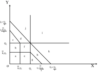
D.1 Six regions giving rise to the total expected profit function . . . 51
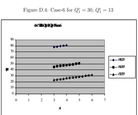
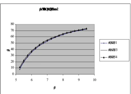
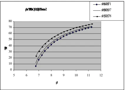
D.2 Eleven regions giving rise to the retailer‘s expected profit function 51 D.3 Case-2 for Qc 1 = 14, Qc1 = 31 . . . 52 D.4 Case-6 for Qc 1 = 30, Qc1 = 13 . . . 52 D.5 Case-2 for Q1 = 13, Q1 = 20 . . . 53 D.6 Case-2 for Q1 = 13, Q1 = 27 . . . 53 D.7 Case-2 for Q1 = 20, Q1 = 20 . . . 54 D.8 Case-2 for Q1 = 20, Q1 = 27 . . . 54 D.9 Case-6 for Q1 = 20, Q1 = 20 . . . 55 D.10 Case-6 for Q1 = 20, Q1 = 27 . . . 55 D.11 Case-6 for Q1 = 27, Q1 = 20 . . . 56 D.12 Case-6 for Q1 = 27, Q1 = 27 . . . 56 ix
E.1 Case-2:One-way full substitution with partial credit and full returns for Qc
1 = 14, Qc2 = 31, d1 = 4.5, d2 = 3 . . . 57
E.2 Case-2:One-way full substitution with partial credit and full returns for Qc
1 = 14, Qc2 = 31, d1 = 6, d2 = 4.5 . . . 58
E.3 Case-2:One-way full substitution with partial credit and full returns for Qc
1 = 14, Qc2 = 31, d1 = 7, d2 = 5.5 . . . 58
E.4 Case-6:Two-way full substitution with partial credit and full returns for Qc
1 = 30, Qc2 = 13, d1 = 4.5, d2 = 3 . . . 58
E.5 Case-6:Two-way full substitution with partial credit and full returns for Qc
1 = 30, Qc2 = 13, d1 = 6, d2 = 4.5 . . . 59
E.6 Case-6:Two-way full substitution with partial credit and full returns for Qc
1 = 30, Qc2 = 13, d1 = 7, d2 = 5.5 . . . 59
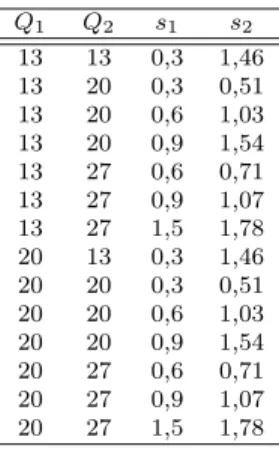
E.7 Parameter sets for case-2 . . . 59 E.8 Parameter sets for case-6 . . . 60 E.9 Case-2a:One-way full substitution with partial credit and full
returns for Q1 = 13, Q2 = 13, s1 = 0.3, s2 = 1.46 . . . 60
E.10 Case-2b:One-way full substitution with partial credit and full returns for Q1 = 13, Q2 = 20 . . . 61
E.11 Case-2c:One-way full substitution with partial credit and full returns for Q1 = 13, Q2 = 27 . . . 61
E.12 Case-2d:One-way full substitution with partial credit and full returns for Q1 = 20, Q2 = 13, s1 = 0.3, s2 = 1.46 . . . 62
E.13 Case-2e:One-way full substitution with partial credit and full returns for Q1 = 20, Q2 = 20 . . . 62
E.14 Case-2f:One-way full substitution with partial credit and full returns for Q1 = 20, Q2 = 27 . . . 63
E.15 Case-6a:Two-way full substitution with partial credit and full returns for Q1 = 20, Q2 = 20 . . . 63
E.16 Case-6b:Two-way full substitution with partial credit and full returns for Q1 = 20, Q2 = 27 . . . 64
E.17 Case-6c:Two-way full substitution with partial credit and full returns for Q1 = 27, Q2 = 20 . . . 64
E.18 Case-6d:Two-way full substitution with partial credit and full returns for Q1 = 27, Q2 = 27 . . . 65
E.19 Manufacturer‘s Profit Margin (MPM)and Retailer‘s Profit Margin(RPM) for product 1 and product 2 . . . 65
Introduction and Literature
Review
Supply chain management and contracts between levels of a supply chain have gained considerable attention in the literature in the last decade. A simple supply chain structure with a single product consists of an upstream party, the manufacturer, and a downstream party, the retailer. The retailer orders the product from the manufacturer in advance of a selling season with stochastic demand. The manufacturer produces after receiving the retailer‘s order and delivers his production to the retailer at the start of the selling season. The manufacturer produces the product at a constant unit cost and charges the retailer a wholesale/transfer payment. The retailer, in turn, sells the product at a unit price. Therefore, supply chain activities begin with a customer order and end when a customer is satisfied.
In this study a simple supply chain structure with a single retailer and a manufacturer, is considered for two perishable products which can be substituted for each other with fixed probabilities. The retailer is also allowed to return some products to the manufacturer according to the contract between the retailer and the manufacturer. The aim is to analyse the system to achieve channel coordination.
There are two main control structures for a supply chain. One of them is the centralized and, the other is the decentralized control structure. Supply chain profit is the total profit to be shared across all supply chain stages. If all decisions are made by a single decision maker with access to all available information, then the total expected supply chain profit is maximized. This is referred to as central control. The resulting total expected profit is described as centralized total expected profit. However, the supply chain members are primarily concerned with optimizing their own objectives. This means neither the manufacturer nor the retailer is in a position to control the entire supply chain, and each has his own incentives and state of information. This is referred to as a decentralized control structure, with resulting decentralized total expected profit.
A main question in supply chain management is how to increase the supply chain performance. The answer to this question helps to understand why the retailer and the manufacturer make certain contract. Optimal supply chain performance requires the execution of a precise set of actions to increase the total supply chain profits. However, those actions are not always in the interest of the members in the supply chain as in the decentralized case, resulting in poor performance.
A contract contains specifications of quantity, price, time and quality. A necessary condition for the adoption of any contractual agreement is that both parties ultimately benefit. One of the advantages of a contract is to share the risk between the retailer and the manufacturer. This is common in contracts. The risk sharing objective focuses on how decentralized total expected profit is to be split between the retailer and the manufacturer. The risks arise from various sources of uncertainty, e.g. market demand, selling price, process yield, product quality, delivery time, and exchange rates. As mentioned in Tsay, Nahmias and Agrawal [23],”suppose that the retailer is required to transmit sales forecasts to the manufacturer. These forecasts are intended to help the manufacturer to make capacity and materials purchasing decisions. However, in most cases no commitment is attached to these forecasts. As a result, the manufacturer assumes a large portion of the risk of demand uncertainty. Not
only might the retailer cancel orders if demand is lower than anticipated, there is an incentive for the retailer to deliberately inflate forecasts as a form of insurance.” Minimum purchase agreements or penalties for returns are often included in contracts to protect the manufacturer against this behavior.
Contracts also facilitate long-term partnerships. Another example given in Tsay [23] is as follows:”Intel might be willing to sell a large portion of its production of a new generation of microprocessors to a single computer maker, such as Dell. The microprocessor may sell for a higher price in open market. However, Intel’s motivation would be to build long-term relationship in the hope that Dell would be a volume purchaser for many years.”
Contracts make the terms of the relationship explicit. Each party’s expectations on lead times, on-time delivery rates and product quality are made legally concrete.
Coordination among the retailer and the manufacturer is a very important issue in supply chain management. Contracts also provide the system-wide performance improvement. The objective is to bring decentralized expected profit closer to centralized expected profit. This is also referred to as the channel coordination objective. If decentralized expected profit is equal to centralized expected profit then the channel efficiency is said to be equal to one. In other words, the customer’s order quantity is equal to the production quantity of a manufacturer that both produces as well as sells the products. The parameter set determination is important to achieve channel coordination. There are many studies in literature related to contracts in supply chain management. The main concepts in these papers can be classified as follows as in Tsay, Nahmias and Agrawal [23]:
• Specification of decision rights • Pricing
• Quantity flexibility
• Buyback or return policies • Allocation rules
The literature review of the above concepts can be seen in the review paper Tsay, Nahmias and Agrawal [23]. Only some papers related to these concepts are referred here. The literature of specification of decision rights can be classified into three groups. Most of the multi-echelon inventory studies of specification of decision rights is on central control, e.g. Clark and Scarf [1], Rosling [12]. Then, the literature is followed by considering how to facilitate the shift from centralized control to decentralized control. (e.g. Lee and Whang [21], Porteus and Whang [14]). Finally, others focus on solutions which transfer decision rights among the various independent agents, see e.g. Blair and Lewis [16]. Another concept is pricing. In most of the traditional inventory models, price paid by the retailer to the manufacturer is fixed. However, more recently, pricing is considered as to be modified by the retailer or both the retailer and the manufacturer. Therefore, both parties have considered the use of quantity discounting as a coordination mechanism discussed in Monahan [8], Lee and Rosenblatt [10]. A main paper considering the role of pricing in channel coordination is by Jeuland and Shugan [6]. They compared the optimality conditions with and without coordination. Other studies with pricing are extensions of this study. In traditional studies, the retailer can order any quantity from the manufacturer at any time. However, this is undesirable from the manufacturer‘s point of view for a variety of reasons. The most important reason is the bullwhip effect. The retailer makes no order for a long time due to waiting for the cumulative demand to become sufficiently large. This causes an increase in demand variance. So, minimum purchase agreement can be a solution to this problem. Moreover, a minimum purchase commitment may also require special pricing terms to attract the retailer. In fact, more than one of these categories are included in many studies. The minimum commitment per period is studied by many researchers, e.g. Anupindi and Akella [15]. In quantity flexibility, the retailer may deviate from the minimum purchase
commitment. Three questions may arise from quantity flexibility: How should the retailer behave given the available flexibility, how should the manufacturer behave given the flexibility promised the retailer and what would be the cost and the benefit to each party of changes to parameters of the agreement. In the literature, these three questions are tried to be answered. The last issue is allocation rules. Allocation issues arise when multiple retailers compete for a product. There are mainly two papers, Cachon and Lariviere [18] and Cachon and Lariviere [19]. Cachon and Lariviere [18] model a single-period, single supplier, multi-retailer supply chain where the supplier‘s production capacity is limited and each retailer‘s stocking level is private information. The other paper considers a one-supplier, retailer supply chain in a two-period environment. These two papers show the effect of allocation on supply chain behavior and performance. But, they do not specify what allocation policies might be optimal.
In Tsay, Nahmias and Agrawal [23], some types of supply contracts are mentioned to coordinate the newsvendor and to divide the supply chain‘s profit. Some examples of contracts are sales rebate contract, quantity flexibility, wholesale price contracts, buyback contract, and revenue sharing contract. Each one coordinates by inducing the retailer to order more than he would with just a wholesale price contract. Quantity flexibility contract induces the retailer by giving the retailer some refund when demand is lower than order quantity. Only some percentage of unsold products can be returned for full credit to the manufacturer in quantity flexibility contract. The sales rebate contract induces the retailer by giving the retailer some incentive when demand is greater than a threshold t. So, the retailer purchases the units sold above threshold t for less than their cost of production. In revenue-sharing contract, the manufacturer gets some credit per unit sold to the retailer plus the retailer gives the manufacturer some percentage of his revenue. In buyback contract, all unsold products can be returned to the manufacturer for partial credit. In fact, revenue sharing is equivalent to buyback contract when some mathematical relationship is satisfied between the percentage shared and the partial credit.
To summarize, there are a large number studies relating to the coordinating contracts. However, it is not easy to set the conditions under which one contract must be preferred over the other. A simple contract is particularly desirable if the contract‘s efficiency is high (the ratio of supply chain profit with the contract to the supply chain‘s optimal profit) and if the contract designer gets the lion‘s share of supply chain profit.
When the number of products that the retailer stocks is large, stock control becomes more difficult. Especially if these products can be substituted for each other with a fixed probability. Moreover, the retailer may return some or all unsold product to the manufacturer, possibly for only partial credit. There are several motivations for a manufacturer to accept a returned product. A manufacturer may want to have a return policy to enhance the retailer for the popularity of his products. Alternatively, a manufacturer may want to accept returns to rebalance inventory among retailers when there are more than one retailer.
Before getting started to explaining the model considered in this study, let us mention about the related literature. There are many papers related to return strategies and substitutability. One of the earliest studies for channel coordination and buyback contracts is Pasternack [9]. In Pasternack [9], a manufacturer produces a single product for sale to a retailer, the product has a relatively short shelf or a demand life, and the retailer places only one order with the manufacturer. The manufacturer sets the wholesale price and the market selling price is fixed, so the only decision for the retailer is the order quantity. The classical newsboy setting is considered, in which the demand is for a single period and the inventory is not carried forward into the future. The single-period inventory model is frequently used to analyze stocking levels for perishable or short shelf-life products. Typical products are newspapers, seasonal items, fashion items, etc. Using a single-period inventory model, Pasternack [9] finds that neither a policy allowing for unlimited returns at full credit, nor the one allowing for no returns is efficient to achieve channel coordination. Pasternack [9] determines that the coordination of the channel can be achieved by a buyback contract allowing for full returns
at a partial credit. The efficient prices can be set in a way that guarantees Pareto improvement. In order to implement an efficient contract, guaranteeing Pareto improvement is necessary in order to insure retailer‘s participation. In Pasternack [9] different channel coordinating prices paid by the retailer to the manufacturer per unit and credits per unit paid by the manufacturer to the retailer per unit for returned products lead to different ways of splitting the channel profit between the manufacturer and the retailer. However, how does or should the manufacturer pick implementable prices is not addressed.
In another paper, Lau [22] suggests a model for designing the pricing and return-credit strategy for a monopolistic manufacturer of single-period products. The manufacturer determines the unit price to be charged from the retailer (C) and the unit credit to be given to the retailer for units returned (V) given the unit manufacturing cost, the unit retail sale price, the risk attitude of himself and the retailer and the demand uncertainty. The order quantity is set by the retailer after taking the manufacturer‘s decisions. Also, retailer has an enforceable minimum profit requirement. The major purpose of the study is to see whether it is desirable from the manufacturer’s perspective to grant return credits and how the manufacturer should coordinate the pairs of credit and price with changing channel efficiencies. These channel efficiencies show how much the channel coordination is achieved. The findings derived from the model are:
• The manufacturer can usually design a C,V that gives himself the lion‘s share of the profit unless an external force supports the retailer
• The optimal return policy can range from ‘no returns allowed‘ to ‘unlimited returns with full credit‘ depending on the risk attitudes of the retailer and the manufacturer.
In another study by Padmanabhan and Png [20], a manufacturer uses a buyback contract to manipulate the competition between retailers. Buyback contract intensifies the degree of competition between the retailers. More intense retail competition means lower retailer prices, greater sales. As a result,
manufacturer gets larger profits. Emmons and Gilbert [24] study buyback contracts with a retail price setting newsvendor. In their study, the retail commit to both a stocking quantity and a price at which to sell a product prior to the selling season. Donohue [27] studies buyback contracts in a model with multiple production opportunities. Also, the model improves demand forecasts. In fact, there are substantial literature on buyback contracts. However, the studies by Pasternack [9] and Lau [22] are more related to our problem.
Regarding the inventory control of substitutable products, one of the early papers is by Ignall and Veinott [2]. They developed conditions under which the myopic solution ( a solution of minimizing expected cost in the current period line) is optimal also in the long run. Their result can be applied to our problem to determine the long run optimum. We do not deal with the difficult multi-period problem. However, if one is interested in the multi-multi-period problem, then it is possible to deal by using the paper of Ignall and Veinott [2]. Their work was extended by Deuermeyer [5]. He studied a multi-product inventory system with interdependent demand , showed that the rate of substitution is age dependent.
McGillivray and Silver [4] investigated the effects of the substitutability on stocking control rules and inventory costs for the case in which all items have the same unit variable cost and shortage penalty. Their model assumed that if an item is out of stock there is a fixed probability of the customer to substitute another available item. They considered the case of total substitutability (probability of substitution equaling one) and compared this with the case of no substitutability to obtain limits on the potential benefits achievable from substitution. Focusing on the two item case they used simulation to develop costs as well as a heuristic approach for establishing order up to levels. Their results indicated that a consequence of full substitutability would be a decrease in the total optimal order quantity. However, substitutability would be of little consequence when the number of substitutable items stocked is low and probabilities that customers will accept substitutes small.
in which substitution occurs in a probabilistic sense. That is, if one good is out of stock but there is a surplus of other good at the end of the period, the substitution will occur with some constant probability. Their model also assumed that revenue received for a good is unaffected by the substitution. They showed that the total profit function is concave for a wide variety of problem parameters and developed necessary conditions for an optimal solution.
Parlar [11] used a game theoretic approach to model two independent decision makers whose products can be substituted if one becomes out of stock. He showed that there exist a Nash equilibrium solution.
Pasternack and Drezner [13] considered a stochastic model for two products which have a single period inventory structure and which can be used as substitutes for each other. Substitution occurs with probability one, but at a different revenue level. They proved that the expected profit function is concave. This allows to find optimum stocking levels for the case of single substitution with that there is no substitution. They found that if revenue obtained from substitution of one product exceeds the other product, one will order more from that product. They demonstrated that for the case of single substitution total optimum order quantities can decrease or increase with the substitution revenue depending on the problem parameters.
Matthews [3] suggested a model for the manufacturer to optimize his stocking strategy for a periodic review/replenishment system for multi-period case. The model was two stage linear program for n items and there was demand transfer among them. Optimal replenishment cycle is taken as constant and known to see how the net profit changes. It is seen that rates of sale depends on primary demands of items, inventory position of other items for a state, and percentage of demand transferring from an out of stock item to an other item.
Drezner, Gurnani and Pasternack [17] presented an economic order quantity model when two products are available and one can be substituted for the other. They considered three cases, when there is no substitution between
the products, when there is full substitution between the products and when there is partial substitution between the products. It is observed that full substitution is never optimal; only partial substitution or no substitution may be optimal. However, they considered the full substitution as the demands for both products are combined to create one order for one product only. This means order quantity of one product is zero. Also, they presented an algorithm to compute the optimal order quantities.
Gurnani and Drezner [25] considered a deterministic nested substitution problem where there are multiple products which can be substituted one for the other. The trade-off in the substitution process is as follows: a cheaper, more generic product can be substituted for a more expensive and less generic product by incurring an extra cost of transformation. On the other hand, less generic product is hold in inventory for higher holding inventory cost. They formulated the problem to determine the optimal run-out times, so to determine the optimal order and substitution quantities.
Smith and Agrawal [26] developed a probabilistic demand model for items capturing the effects of substitution and a methodology for selecting item inventory models so as to maximize total expected profit, subject to given resource constraints. Inventory optimization includes both the selection of which items to stock and the stock levels for each item. They gave examples to see the behavior of the optimal inventory policies, using negative binomial demand distribution. The major insights are as follows: optimal assortment and inventory levels are significantly effected by substitution; policies derived from ignoring substitution effects can be less profitable than those that incorporating substitution effects; substitution effects can reduce the optimal assortment size and with substitution effects, it is not always optimal to stock the most popular items, even when all items are equally profitable.
In this thesis, we consider a simple supply chain structure with a retailer and a manufacturer, for two substitutable products According to the contract between the manufacturer and the retailer, the retailer is allowed to return some unsold products to the manufacturer. General expressions are derived for the
expected total profit of the supply chain, the expected profit of the retailer and the expected profit of the manufacturer. Some special cases, regarding the substitution probabilities and return proportions are considered to obtain the necessary conditions for channel coordination. Negative binomial distribution is considered for numerical studies.
It is found that when substitutability is concerned either one-way or two-way full substitution (a policy of allowing for unlimited returns for partial credit) is system optimal. As in Pasternack [9], it is observed that full credit full return contracts can not achieve system coordination.
Organization of the thesis is as follows:
In Chapter 2, the general model is introduced and the expected profit expressions are provided. In Chapter 3, special cases are considered and necessary conditions to achieve channel coordination are obtained. Results of our numerical study are presented in Chapter 4. Finally, in Chapter 5 concluding remarks are made and future research directions are stated.
General Model
In this study, we consider a single period newsboy type inventory problem with two substitutable products in a two level supply chain, consisting of a retailer and a manufacturer.
Among several contract types that are discussed in the literature, we focus on the case where the retailer is allowed to return some or all of the unsold products to the manufacturer with partial or full credit. Our set-up is similar to that of Pasternack [9] except that we generalize his study for two substitutable products.
We first derive the expressions for the total expected channel profit, manufacturers expected profit and the retailer‘s expected profit under general model parameters. We then investigate the special cases for channel coordination. In particular, we say that coordination is achieved if the retailer‘s order quantity is the same as the production quantity of the manufacturer that both produces and directly sells to the market as in Pasternack [9].
Throughout the study we assume that the original demand to each product is satisfied first. If there is excess inventory from one product and there is excess demand in the other, a portion of this excess demand is satisfied from the other available product.
Let us first introduce the notation. For product i, i = 1, 2; the manufacturing cost is ci and di is the price paid by the retailer to the
manufacturer. Credit paid by the manufacturer to the retailer for returned item i is denoted by si. Qi is the order quantity for product i to be determined
by the retailer. The percentage of the order quantity Qi which the retailer
can return to the manufacturer for a credit of si per item i is Ri. X is the
random demand for item 1 with density (or probability mass function) f (x) and distribution function F (x). Y is the random demand for item 2 with density (or probability mass function) g(y) and distribution function G(y). A customer will accept a unit of item 2 when item 1 is out of stock with probability a for sale price p2. The probability of accepting a unit of item 1 when item 2 is out
of stock for a sale price p1 is b. We also assume that;
ci ≤di ≤pi (1)
There is no salvage cost and goodwill cost unlike in Pasternack(11). In the following sections, the expressions for the expected total supply chain profit, the retailer‘s expected profit and the manufacturer‘s expected profit are obtained.
2.1
Total Supply Chain Expected Profit
Using the above notation and the assumptions, we aim to derive the expression for the total expected profit of the supply chain, which will be denoted by EPT(Q1, Q2). Total expected profit of the supply chain is obtained by
considering the case where the producer sells the products directly to the customer and is not involved in any contracts with a retailer.
Note that, initially, when Q1,Q2 units are produced, a cost of c1Q1+ c2Q2
is incurred. In addition, we have considered six profit expressions πa, πb,
πc, πd, πe, πf over their respective regions when respective demands (X =
for EPT(Q1, Q2) can be more easily followed by referring to Figure D.1 in
Appendix-D.
In region a, demands for both products are less than their inventory levels and profit expression is;
πa = p1x+ p2y x ≤ Q1, y ≤ Q2 (a)
In region b, demand for product 1 exceeds its inventory level but the excess demand can be fully satisfied by product 2 and profit expression is;
πb = p2y+ p2a(x − Q1) + p1Q1 x ≥ Q1, y ≤ Q2, a(x − Q1) < Q2−y (b)
In region c, demand for product 1 exceeds its inventory level and the excess demand can only be partially satisfied by product 2 and profit expression is;
πc= p1Q1+ p2Q2 x ≥ Q1, y ≤ Q2, a(x − Q1) > Q2−y (c)
In region d, demands for both products are greater than their inventory levels and profit expression is;
πd = p1Q1+ p2Q2 x ≥ Q1, y ≥ Q2 (d)
In region e, demand for product 2 exceeds its inventory level and the excess demand can only be partially satisfied by product 1 and profit expression is;
πe = p1Q1+ p2Q2 x ≤ Q1, y ≥ Q2, Q1−x < b(y − Q2) (e)
In region f , demand for product 2 exceeds its inventory level and can be fully satisfied by product 1 and profit expression is;
πf = p1x+ p1b(y − Q2) + p2Q2 x ≤ Q1, y ≥ Q2, Q1 −x > b(y − Q2) (f)
Total supply chain expected profit expression, EPT(Q1, Q2), is obtained by
integrating these profit expressions over their respective regions plus −c1Q1−
Proposition 2.1.1:
Under the assumed model, the total expected profit of the supply chain is given by: EPT(Q1, Q2) = −p1 Z Q1 0 F(x)G(Q2+ (Q1−x) b )d(x) + (p2−c2)Q2 − p2 Z Q2 0 G(x)F (Q1+ (Q2−x) a )d(x) + (p1−c1)Q1 (1)
2.2
Retailer‘s Expected Profit
We consider a hierarchical situation in which the retailer determines the order quantity to purchase from the manufacturer. The retailer‘s expected profit, EPR(Q1, Q2), is derived below. The derivation is based on considering the
profit in several realizations as seen in Figure D.2 in Appendix-D.
Suppose the retailer orders Q1 and Q2 units of products with a cost given
by d1Q1+ d2Q2. We consider the profit in eleven possible regions from a to k
according to the realized demand (X = x, Y = y).
In region a , x ≤ (1 − R1)Q1, y ≤(1 − R2)Q2, demand for product 1 is less
than (1 − R1).Q1 and demand for product 2 is less than (1 − R2).Q2 and unsold
ones are returned to the manufacturer for the permitted return percentage R1
and R2 and profit expression is;
πa = p1x+ p2y+ R1Q1s1+ R2Q2s2 (a)
In region b, x ≤ (1 − R1)Q1,(1 − R2)Q2 ≤y ≤ Q2, demand for product 1 is
less than (1 − R1).Q1 and demand for product 2 is in between (1 − R2).Q2 and
Q2) and unsold product 1 is returned for permitted return percentage R1), all
unsold product 2 are returned to the manufacturer and profit expression is; πb = p1x+ p2y+ R1Q1s1+ (Q2 −y)s2 (b)
2 exceeds its inventory level but the excess demand can be fully satisfied by product 1 and R1.Q1 amount of product 1 is returned to the manufacturer and
profit expression is;
πc= p1x+ p1(b(y − Q2)) + R1Q1s1+ p2Q2 (c)
In region d, y ≥ Q2, Q1 −(x + b(y − Q2)) < R1Q1, x+ b(y − Q2) < Q1,
demand for product 2 exceeds its inventory level but the excess demand can be fully satisfied by product 1 and all unsold amount of product 1 is returned to the manufacturer, and profit exxpression is;
πd = p2Q2+ p1(x + b(y − Q2)) + (Q1−x − b(y − Q2))s1 (d)
In region e, y ≤ (1 − R2)Q2,(1 − R1)Q1 ≤ x ≤ Q1, demand for product
1 is in between (1 − R1).Q1 and Q1) and for product 2 demand is less than
(1 − R2).Q2 and all unsold product 1, R2.Q2 amount of product 2 are returned
to the manufacturer, and profit expression is; πe = p1x+ p2y+ R2Q2s2+ (Q1−x)s1 (e)
In region f , (1−R1)Q1 ≤x ≤ Q1,(1−R2)Q2 ≤y ≤ Q2, demand for product
1 is in between (1−R1).Q1 and Q1) and for product 2 is in between (1−R2).Q2
and Q2) and all unsold product 1 and 2 are returned to the manufacturer, and
profit expression is;
πf = p1x+ p2y+ (Q1−x)s1+ (Q2 −y)s2 (f)
In region g, x ≥ Q1, Q2 −(y + a(x − Q1)) > R2Q2, demand for product
1 exceeds its inventory level but the excess demand can be fully satisfied by product 2 and R2.Q2 amount of product 2 is returned to the manufacturer,
and profit expression is;
πg = p2y+ p2(a(x − Q1)) + R2Q2s2+ p1Q1 (g)
In region h, x ≥ Q1, Q2 −(y + a(x − Q1)) < R2Q2, y+ a(x − Q1) < Q2,
demand for product 1 exceeds its inventory level but the excess demand can be fully satisfied by product 2 and all unsold amount of product 2 is returned
to the manufacturer, and profit expression is;
πh = p1Q1+ p2(y + a(x − Q1)) + (Q2−y − a(x − Q1))s2 (h)
In region i, x ≥ Q1, y ≥ Q2, demands for both products are greater than
their inventory levels, and profit expression is; πi = p1Q1 + p2Q2 (i)
In region j, y ≥ Q2, x+ b(y − Q2) < Q1, x < Q1, demand for product 2
exceeds its inventory level and the excess demand can only be partially satisfied by product 1, and profit expression is;
πj = p1Q1+ p2Q2 (j)
Finally, in region k, x ≥ Q1, y + a(x − Q1) < Q2, y < Q2, demand for
product 1 exceeds its inventory level and the excess demand can only be partially satisfied by product 2, and profit expression is;
πk = p1Q1+ p2Q2 (k)
Retailer‘s expected profit expression, EPR(Q1, Q2), is obtained by
integrat-ing these profit expressions over their respective regions plus −d1Q1 −d2Q2.
The proof of this expression is given in the Appendix B. Proposition 2.2.1:
Under the assumed buyback and return contract the retailers expected profit is given by:
EPR(Q1, Q2) = − p1 Z Q1 0 F(x)G(Q2+ (Q1−x) b )d(x) + (p2−d2)Q2 − p2 Z Q2 0 G(x)F (Q1+ (Q2−x) a )d(x) + (p1−d1)Q1 + F (Q1)s2 Z Q2 R2Q2 G(y)d(y) + G(Q2)s1 Z Q1 R1Q1 F(x)d(x) + Z ∞ Q2 Z Q1−b(y−Q2) R1Q1−b(y−Q2) [Q1−x − b(y − Q2)]s1dF(x)dG(y)
+ R1Q1s1 Z Q2+(R1Q1)b Q2 F(R1.Q1−b(y − Q2))dG(y) + Z ∞ Q1 Z Q2−a(x−Q1) R2Q2−a(x−Q1) [Q2−y − a(x − Q1)]s2dG(y)dF (x) + R2Q2s2 Z Q1+(R2Q2)a Q1 G(R2Q2−a(x − Q1))dF (x) (2)
In the above expressions Ri = 1 − Ri, i = 1, 2.
2.3
Manufacturer Expected Profit
Now, we consider the expected profit of the manufacturer under the buyback contract with the retailer. Figure D.2 in Appendix-D can also be used to derive the expected profit of the manufacturer. The paid money to the retailer for returned products are calculated for each subcases. Then the derivation, EPM(Q1, Q2), is based on considering the profit earned Q1(d1−c1)+Q2(d2−c2)
minus the money paid to retailer for returned products calculated in each region in Figure D.2 in Appendix-D.
Note that since
EPT(Q1, Q2) = EPR(Q1, Q2) + EPM(Q1, Q2)
We have
EPM(Q1, Q2) = EPT(Q1, Q2) − EPR(Q1, Q2)
However, for verification purposes we also separately derived this expression as described below.
We have the following expressions for the money paid back to the retailer in different regions;
πa = R1Q1s1+ R2Q2s2 (a)
πc= R1Q1s1 (c) πd = (Q1−x − b(y − Q2))s1 (d) πe = R2Q2s2+ (Q1−x)s1 (e) πf = (Q1−x)s1+ (Q2−y)s2 (f) πg = R2Q2s2 (g) πh = (Q2−y − a(x − Q1))s2 (h)
In region i, j and k no money is returned to the retailer. Therefore, we have:
πi = πj = πk = 0
Manufacturer‘s expected profit, EPM(Q1, Q2), is obtained by subtracting
the total integrated profit expressions over their respective regions from Q1(d1−
c1) + Q2(d2−c2) as follows:
Proposition 2.3.1:
Under the buyback and return contracts, the manufacturer‘s expected profit is given by: EPM(Q1, Q2) = (d1−c1)Q1+ (d2−c2)Q2 − F(Q1)s2 Z Q2 R2Q2 G(y)d(y) − G(Q2)s1 Z Q1 R1Q1 F(x)d(x) − Z ∞ Q1 Z Q2−a(x−Q1) R2Q2−a(x−Q1) [Q2−y − a(x − Q1)]s2dG(y)dF (x) − R1Q1s1 Z Q2+(R1Q1)b Q2 F(R1Q1 −b(y − Q2))dG(y) − Z ∞ Q1 Z Q2−a(x−Q1) R2Q2−a(x−Q1) [Q2−y − a(x − Q1)]s2dG(y)dF (x) − R2Q2s2 Z Q1+(R2Q2) a Q1 G(R2Q2−a(x − Q1))dF (x) (3)
Special Cases
In this section, we consider several special cases and investigate the conditions under which channel coordination is achieved.
We mainly focus on special cases in terms of the return fractions, substitution probabilities and credits paid for the returned items. Several cases corresponding to full or partial credits; full or partial substitution among the two products and one-way or two-way substitution are inspected separately. In all the special cases we use the same approach for finding the conditions under which the channel coordination is achieved. Firstly, total supply chain expected profit, EPT(Q1, Q2) , and retailer‘s expected profit, EPR(Q1, Q2), are written
for the special values of a, b, R1, R2. Then the conditions are investigated for
which the optimal order quantities that maximize EPR(Q1, Q2) are equal to
the production quantities of the manufacturer that maximize EPT(Q1, Q2).
In the following discussions we assume that EPT(Q1, Q2) is unimodal in
(Q1, Q2), so that there exist a unique (Qc1, Qc2) that maximizes the channel
profit EPT(Q1, Q2). Concavity of the total profit function is proved by Parlar
and Goyal [7]. Hence the analysis is based on the first order conditions. Namely, the conditions under which (Qc
1, Qc2) becomes equal to the optimal
order quantities of the retailer are investigated. In some special cases of the contracts, the first order conditions of the retailer is satisfied only when order
quantities are infinite, and in this case we say that the system is sub-optimal. Otherwise if the first order conditions are satisfied at finite order quantities, we assume that they are also optimal quantities. Similarly, when infeasible conditions are required for the channel coordination, (such as zero profit of the manufacturer or the retailer) we refer to this as system sub-optimality.
3.1
Case-1:
Full returns with partial credit
and no substitution
Suppose the retailer is allowed to return all unsold products to the manufacturer and there is no substitution between the two products then we have the following results;
Proposition 3.1.1 :
Let a = 0, b = 0, R1 = R2 = 1 and Qc1, Qc2 be the optimal production
quantities of the manufacturer. Then channel coordination is achieved if the following condition is satisfied.
p1−c1 p1 = p1−d1 p1−s1 = F (Qc 1) (1) p2−c2 p2 = p2−d2 p2−s2 = G(Qc2) (2) Proof:
If the manufacturer produces Q1, Q2 and sells to the public directly his
expected profit, EPT(Q1, Q2), will be given by:
EPT(Q1, Q2) =-p1
RQ1
0 F(x)d(x) + (p2−c2)Q2-p2
RQ2
0 G(y)d(y) + (p1−c1)Q1
Setting the derivatives with respect to Q1 and Q2 equal to zero, we obtain;
0 = p2−c2−p2G(Qc2) (4)
Note that the second derivatives are given by −p1f(Q1) and −p2f(Q2) which
indicates that EPT(Q1, Q2) is concave in Q1, Q2. For this special case we also
have; EPR(Q1, Q2) = − p1 Z Q1 0 F(x)d(x) + (p2−d2)Q2 − p2 Z Q2 0 G(y)d(y) + (p1 −d1)Q1 + F (Q1)s2 Z Q2 0 G(y)d(y) + G(Q2)s1 Z Q1 0 F(x)d(x) + Z ∞ Q2 Z Q1 0 [Q1 −x]s1dF(x)dG(y) + Z ∞ Q1 Z Q2 0 [Q2 −y]s2dG(y)dF (x)
When the derivatives are set to zero, we have;
0 = p1−d1−p1F(Q1) + s1F(Q1) (5)
0 = p2−d2−p2G(Q2) + s2G(Q2) (6)
The second derivatives are obtained as −(p1−s1)f (Q1) and −(p2−s2)g(Q2)
respectively and their non-negativity imply the concavity of the retailer‘s profit. Solving (3), (4), (5) and (6) simultaneously results in;
p1−c1 p1 = p1−d1 p1−s1 = F (Qc1) p2−c2 p2 = p2−d2 p2−s2 = G(Qc2) Remarks:
1- When there is no substitution as in this case, the result for two product is same as obtained for one product in Pasternack(11), except that we have two independent products.
2- The policy of a manufacturer allowing unlimited returns for full credit is system suboptimal.
3- The policy of a manufacturer allowing no returns is system suboptimal 4- A policy of which allows for unlimited returns at partial credit will be system optimal for appropriately chosen values of p1, c1, d1, s1, p2, c2, d2 and s2
as the condition above (1) and (2)
3.2
Case-2:
Full returns with partial credit
and one-way full substitution
Now, we consider the following special case: The retailer returns all unsold products to the manufacturer with partial credit and only one of the products is substituted with the other with certainty. Then, we have the following result;
Proposition 3.2.1:
Let a = 1, b = 0, R1 = 1 and R2 = 1. Then, to achieve channel coordination
the following equality must hold:
F(Qc1) = c2(p2−s2) + p2(s2−d2+ d1−c1) + s2(p1+ c1) s1p2−s2p1 (7) provided that 0 < c1−c2 < p1 (8) where Qc
1 is the centralized solution that satisfies (9) and (10)
Proof:
In this case, EPT(Q1, Q2) , will be given by:
EPT(Q1, Q2) = − p1. Z Q1 0 F(x).d(x) + (p2 −c2).Q2 − p2. Z Q2 0 G(y).F (Q1+ Q2 −y).d(y) + (p1 −c1).Q1
For the partial derivatives we use the Leibniz‘s rule below; d dt Z β(t) α(t) F(x, t)d(x) = F (β(t), t).β 0 (t) − F (α(t), t).α0(t) + Z βt α(t)[ σF(x, t) σt ]d(x) Setting the first partial derivatives of EPT(Q1, Q2) to zero we obtain;
0 = p1−c1−p1F(Qc1) − p2. Z Qc2 0 G(y).f (Q c 1+ Qc2−y).d(y) (9) 0 = p2−c2−p2G(Qc2)F (Q c 1) − p2. Z Qc2 0 G(y).f (Q c 1+ Q c 2−y).d(y) (10)
From which we obtain; 1 − F (Qc
1)G(Qc2) =
c2 + p1−c1−F(Qc1)p1
p2
(11)
Note that in order that (11) is satisfied and feasible (8) must hold.
For this special case the retailer‘s expected profit, EPR(Q1, Q2), will be
given by : EPR(Q1, Q2) = − p1. Z Q1 0 F(x).d(x) + (p2−d2).Q2 − p2. Z Q2 0 F(Q1+ Q2 −y).G(y).d(y) + (p1 −d1).Q1 + F (Q1).s2 Z Q2 0 G(y).d(y) + G(Q2).s1 Z Q1 0 F(x).d(x) + Z ∞ Q2 Z Q1 0 [Q1 −x]s1dF(x)dG(y) + Z ∞ Q1 Z Q1+Q2−x Q1−x [Q2−y+ Q1−x]s2dG(y)dF (x)
The partial derivatives set to zero result in: 0 = − p1F(Q1) + p1−d1+ s1F(Q1) − p2. Z Q2 0 f(Q1+ Q2 −y).G(y).d(y) + Z ∞ Q1 Z Q1+Q2−x Q1−x s2dG(y)dF (x) (12) 0 = − p2. Z Q2 0 f(Q1+ Q2 −y).G(y).d(y) − p2F(Q1)G(Q2) + p2−d2+ s2F(Q1)G(Q2) + Z ∞ Q1 Z Q1+Q2−x Q1−x s2dG(y)dF (x) (13)
Solving (9), (12), (10) and (13) results in; 0 = s1F(Q1) + Z ∞ Q1 Z Q1+Q2−x Q1−x s2dG(y)dF (x) + c1−d1 (14) 0 = s2F(Q1)G(Q2) + Z ∞ Q1 Z Q1+Q2−x Q1−x s2dG(y)dF (x) + c2−d2 (15)
From which we obtain; F(Qc
1)[s1−s2G(Qc2)] = c2−d2−(c1−d1) (16)
(11) and (16) result in (7).
3.3
Case-3: One-way full substitution with no
returns
We now consider the special case with a = 1, b = 0, R1 = R2 = 0.
Proposition 3.3.1:
Under one-way full substitution with no returns R1 = 0 and R2 = 0,
channel coordination requires c1 = d1 and c2 = d2. Hence, the system is
suboptimal, unless the manufacturer makes zero profit. Proof:
In this case, EPT(Q1, Q2) , is given by:
EPT(Q1, Q2) = − p1. Z Q1 0 F(x).d(x) + (p2−c2).Q2 − p2. Z Q2 0 G(y).F (Q1+ Q2 −y).d(y) + (p1 −c1).Q1
From this expression we obtain; 0 = p1−c1 −p1F(Qc1) − p2. Z Qc2 0 G(y).f (Q c 1+ Qc2−y).d(y) (17) 0 = p2−c2 −p2G(Qc2)F (Q c 1) − p2. Z Qc2 0 G(y).f (Qc1+ Qc2−y).d(y) (18)
Also, we have; EPR(Q1, Q2) = − p1. Z Q1 0 F(x).d(x) + (p2−d2).Q2 − p2. Z Q2 0 F(Q1 + Q2−y).G(y).d(y) + (p1−d1).Q1 and; 0 = p1−d1−p1F(Q1) − p2 Z Q2 0 f(Q1+ Q2−y).G(y).d(y) (19) 0 = p2−d2−p2F(Q1)G(Q2) − p2 Z Q2 0 f(Q1+ Q2 −y).G(y).d(y) (20)
Equations (17), (19), (18) and (20) imply that c1 = d1, c2 = d2 which is not
feasible.
3.4
Case-4: Full returns with full credit and
one-way full substitution
This is a special case of case-2 where s1 = d1, s2= d2.
Proposition 3.4.1:
Suppose a = 1, b = 0, R1 = 1, R2 = 1, s1 = d1 and s2 = d2. Then the
system is suboptimal. Proof:
This is a special case of case 2. Consider expressions given by (12) and (13) for the first order conditions of the retailer‘s profit. Letting s1 = d1, s2 = d2,
(12) and (13) becomes; 0 = (p1−s1)(1 − F (Q1)) − p2 Z Q2 0 f(Q1+ Q2 −y)G(y)d(y) + s2 Z ∞ Q1 G(Q1+ Q2−x)dF (x) (21)
0 = (p2−s2)(1 − F (Q1)G(Q2)) − p2 Z Q2 0 f(Q1+ Q2 −y)G(y)d(y) + s2 Z ∞ Q1 G(Q1+ Q2−x)dF (x) (22) Noting that Z Q2 0 f(Q1+ Q2 −y)G(y)d(y) = Z Q1+Q2 Q1 G(Q1+ Q2−u)f (u)d(u) (22) is equivalent to 1 − F (Q1)G(Q2) = Z Q1+Q2 Q1 G(Q1+ Q2−u)dF (u) ≤ Z ∞ Q1 dF(u) = 1 − F (Q1)
which is impossible since 1 − F (Q1)G(Q2) ≥ 1 − F (Q1) except when Q1 =
Q2 = ∞. Hence, the first order conditions of the retailer are satisfied only for
infinite order quantities.
3.5
Case-5: Two-way full substitution with no
returns
We now consider the special case with a = 1, b = 1, R1 = R2 = 0.
Proposition 3.5.1:
Suppose a = 1, b = 1, R1 = 0 and R2 = 0. Then to achieve the channel
coordination the following condition should be satisfied: c1 = d1
c2 = d2
So, the policy of a manufacturer allowing no returns with two-way full substitution is system suboptimal, unless the manufacturer makes zero profit.
Proof:
In this case, EPT(Q1, Q2) , will be given by:
EPT(Q1, Q2) = − p1. Z Q1 0 F(x).G(Q1+ Q2 −x)).d(x) + (p2−c2).Q2 − p2. Z Q2 0 G(y).F (Q1+ Q2 −y).d(y) + (p1−c1).Q1
Then we have the following conditions for optimality; 0 = p1−c1−p1F(Qc1)G(Qc2) − p2. Z Qc2 0 G(y).f (Q c 1+ Qc2−y).d(y) −p1. Z Qc1 0 F(x).g(Q c 1+ Q c 2−x).d(x) (23) 0 = p2−c2−p2G(Qc2)F (Qc1) − p2. Z Qc2 0 G(y).f (Q c 1+ Qc2−y).d(y) −p1. Z Qc1 0 F(x).g(Qc 1+ Qc2−x).d(x) (24) Also, EPR(Q1, Q2) = − p1. Z Q1 0 F(x).G(Q1+ Q2 −x).d(x) + (p2−d2).Q2 − p2. Z Q2 0 G(Q1 + Q2 −y).G(y).d(y) + (p1−d1).Q1
and after differentiating;
0 = p1−d1−p1F(Q1)G(Q2) − p2. Z Q2 0 f(Q1+ Q2 −y).G(y).d(y) −p1. Z Q1 0 g(Q1+ Q2 −x).F (x).d(x) (25) 0 = p2−d2−p2F(Q1)G(Q2) + −p2. Z Q2 0 f(Q1+ Q2−y).G(y).d(y) −p1. Z Q1 0 g(Q1+ Q2 −x).F (x).d(x) (26)
By using the equations (23), (24), (25) and (26) we found the following equations to achieve the channel coordination :
c1 = d1
So, the policy of a manufacturer allowing no returns with two-way full substitution is system suboptimal.
3.6
Case-6: Full return with partial credit and
two-way full substitution
Now, we consider the following special case:
The retailer returns all unsold products to the manufacturer with partial credit and two of the products are substituted with each other with certainty. Then we have the following result;
Proposition 3.6.1:
Let a = 1, b = 1, R1 = 1 and R2 = 1. Then the following conditions should
be satisfied to achieve channel coordination: c2−p2−(c1−p1)
p1 −p2 =
c2−d2−(c1−d1)
s1−s2 (27) provided that both sides of the inequality are between zero and one. This means that if c1 < c2 then p1 < p2.
Proof:
In this case, EPT(Q1, Q2) , will be given by:
EPT(Q1, Q2) = − p1. Z Q1 0 F(x).G(Q1+ Q2 −x).d(x) + (p2−c2).Q2 − p2. Z Q2 0 G(y).F (Q1+ Q2 −y).d(y) + (p1−c1).Q1 By differentiating EPT(Q1, Q2); 0 = p1−c1−p1F(Qc1)G(Qc2) − p2. Z Qc2 0 G(y).f (Q c 1+ Qc2−y).d(y) −p1. Z Qc1 0 F(x).g(Qc1+ Qc2−x).d(x) (28)
0 = p2−c2−p2F(Qc1)G(Q c 2) − p2. Z Q2 0 G(y).f (Q c 1+ Q c 2−y).d(y) −p1. Z Qc1 0 F(x).g(Q c 1+ Qc2−x).d(x) (29)
By using (28) and (29) we obtain the following condition for the central decision maker to maximize his revenues.
F(Qc
1)G(Qc2) =
c2+ p1−c1−p2
p1−p2 (30)
For this special case the retailer‘s expected profit, EPR(Q1, Q2), will be
given by the following formula : EPR(Q1, Q2) = − p1. Z Q1 0 F(x).G(Q1+ Q2−x).d(x) + (p2−d2).Q2 − p2. Z Q2 0 F(Q1+ Q2−y).G(y).d(y) + (p1 −d1).Q1 + F (Q1).s2 Z Q2 0 G(y).d(y) + G(Q2).s1 Z Q1 0 F(x).d(x) + Z ∞ Q2 Z Q1+Q2−y Q2−y [Q1 + Q2−x − y]s1dF(x)dG(y) + Z ∞ Q1 Z Q1+Q2−x Q1−x [Q2−y+ Q1−x]s2dG(y)dF (x)
To find the optimal order quantity for the retailer, Q1, Q2 , we differentiate
EPR(Q1, Q2) with respect to Q1, Q2 and set this amount equal to 0. This gives
the following two expressions:
0 = − p1F(Q1)G(Q2) + p1−d1+ s1F(Q1)G(Q2) − p2. Z Q2 0 f(Q1+ Q2−y).G(y).d(y) + Z ∞ Q2 Z Q1+Q2−y Q2−y s1dF(x)dG(y) + Z ∞ Q1 Z Q1+Q2−x Q1−x s2dG(y)dF (x) − p1. Z Q1 0 F(x).g(Q1+ Q2−x).d(x) (31) 0 = − p2F(Q1)G(Q2) + p2−d2+ s2F(Q1)G(Q2)
− p2. Z Q2 0 f(Q1+ Q2 −y).G(y).d(y) + Z ∞ Q2 Z Q1+Q2−y Q2−y s1dF(x)dG(y) + Z ∞ Q1 Z Q1+Q2−x Q1−x s2dG(y)dF (x) − p1. Z Q1 0 F(x).g(Q1+ Q2−x).d(x) (32)
Moreover, the following condition found from the equations (28), (29), (31) and (32) should be satisfied:
F(Qc
1)G(Qc2) =
c2−d2−(c1 −d1)
s1−s2
(33)
provided that right hand side of (33) is in (0,1). (30) and (33) result in (27).
Remarks:
• Result in Proposition 3.6.1 indicates that the channel coordinating parameters are distribution free. That is they are independent of the demand distributions.
• Channel coordination requires that if the profit of the manufacturer for product i is higher than that for product j, then it must hold that si > sj
and the difference between the profits of the two products must ne less than the difference between the return credits. These are quantified by the conditions di−ci > dj−cj, si > sj and (di−ci) + (dj−cj) < si−sj.
3.7
Case-7: Full return with full credit and
two-way full substitution
Proposition 3.7.1:
Let a = 1, b = 1, R1 = 1, R2 = 1, s1 = d1 and s2 = d2.
Then the system is suboptimal. Proof:
When s1 = d1, s2 = d2, (31) and (32) becomes;
0 = − p2. Z Q2 0 f(Q1+ Q2 −y).G(y).d(y) + (p1−s1)(1 − F (Q1)G(Q2)) + Z ∞ Q2 s1F(Q1+ Q2−y)dG(y) + Z ∞ Q1 s2G(Q1+ Q2−y)dF (y) − p1 Z Q1 0 F(x).g(Q1+ Q2 −x).d(x) (34) 0 = − p2. Z Q2 0 f(Q1+ Q2 −y).G(y).d(y) + (p2−s2)(1 − F (Q1)G(Q2)) + Z ∞ Q2 s1F(Q1+ Q2−y)dG(y) + Z ∞ Q1 s2G(Q1+ Q2−y)dF (y) − p1 Z Q1 0 F(x).g(Q1+ Q2−x).d(x) (35) Note; Z ∞ Q2 F(Q1+ Q2 −y)dG(y) = Z Q1 0 F(x)g(Q1+ Q2−x).d(x) Z ∞ Q1 G(Q1+ Q2−y)dF (y) = Z Q2 0 G(x)f (Q1+ Q2 −x).d(x) Hence, (34) becomes; 0 = − (p2−s2) Z Q2 0 f(Q1+ Q2−y)G(y)d(y) + (p1−s1)(1 − F (Q1)G(Q2)) − (p1−s1) Z Q1 0 F(x)g(Q1+ Q2 −x)d(x)
which implies; 1 = Z Q1 0 G(Q1+ Q2 −y)dF (y) + p2−s2 p1−s1 Z Q2 0 f(Q1+ Q2 −y)G(y)d(y) = Z Q1 0 G(Q1+ Q2 −y)dF (y) + p2−s2 p1−s1 Z ∞ Q1 G(Q1+ Q2−y)dF (y)
adding and subtracting R∞
Q1G(Q1+ Q2−y)dF (y) we obtain;
1 = Z ∞ 0 G(Q1+ Q2 −y)dF (y) + [p2−s2 p1−s1 −1] Z ∞ Q1 G(Q1+ Q2−y)dF (y) = P (X + Y < Q1+ Q2) + [ p2−s2 p1−s1 −1]P (X + Y < Q1+ Q2, X > Q1) (36)
If p2−s2 < p1−s1, then (36) is not satisfied unless Q1 = Q2 = ∞.
Similarly, we can show that (35) can be written as; 1 = Z Q2 0 F(Q1+ Q2 −y)dG(y) + p1−s1 p2−s2 Z Q1 0 g(Q1+ Q2 −y)F (y)d(y) (37)
Using the same argument as above, we see that if p1 −s1 < p2 −s2 then
(37) can not be satisfied unless Q1 = Q2 = ∞.
Hence (36) and (37) hold simultaneously only if Q1 = Q2 = ∞, and the
Numerical Studies
In this chapter, we present the results of our numerical study. We have done the numerical studies for case-2 and case-6 as described in Chapter-3. In all these cases, where coordination is achieved, we have R1 = R2 = 1. Substitution
probabilities (a,b) for the two products are, either 0 or 1. Therefore, effect of substitution on coordination can be seen in the results. Demand distribution for both products, is taken as negative binomial with parameters ri : 5, pi :
0.25, i=1,2. Note that, if Y is a negative binomial random variable then the probability mass function p(y), variance V (Y ) and the expectation E(Y ) are as follows. For 0 < p < 1; p(y) = y −1 r −1 pr(1 − p)y−r y= r, r + 1, ....for 0 < p < 1 E(Y ) = r p V(Y ) = r(1 − p) p2 34
4.1
Channel Coordinating Transfer Payments
and Buyback Credits
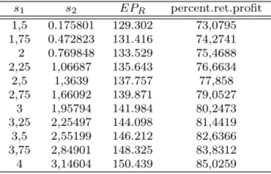
In this part of the numerical study we consider case 2 and case 6 and investigate the coordinating values of the transfer payments d1, d2, and the buyback credits
s1, s2. To this end, as we indicated above, we first set c1 = 3, c2 = 2, p1 = 9 and
p2 = 7 and searched for the optimal production quantity of the manufacturer
by maximizing the expression, EPT(Q1, Q2), for the channel profit. We denote
the optimal quantities by Qc
1, Qc2. We then searched for the transfer payments
and buyback credits that achieve channel coordination using the results of Proposition 3.2.1 and 3.6.1. The results for case 2 are provided in Tables E.1 to E.3. The optimal quantities are found as Q1 = 14 and Q2 = 31. This shows
that the inventory level of the good which is substituted for the other product 2 is greater than the other product, as expected. Moreover, we have found that the total expected chain profit, EPT(Q1, Q2) is 177.808. Similarly, the results
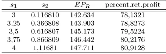
for case 6 is provided in Tables E.4 to E.6. The optimal quantities for this case are Q1 = 30 and Q2 = 13. Similar to case 2 the quantity of product 1 is greater
than that of product 2. This is explained by the fact that the price of product 1 (p1 = 9) is greater than the price of product 2 (p2 = 7). Total expected chain
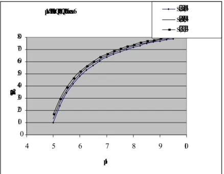
profit for case 6 is found as 183.539 which is greater than the profit in case-2. This is understandable, since in case 6, substitution occurs in both direction. As d1, d2 increase, manufacturer‘s profit increase. When we compare Tables
E.1 to E.3 and E.4 to E.6 we see that as d1, d2 increase, the percentage share
of the retailer decrease substantially as expected. On the other hand, as s1, s2
increase, the retailer‘s profit and share also increase. As manufacturer‘s profit margin for both products increases, see Table E.19, then retailer‘s profit share decreases as seen in Tables E.9, E.10, E.11, E.12, E.13 and E.14. At the same time, wee see that retailer‘s profit margin decreases as manufacturer‘s profit margin increases.
4.2
Further Analysis with Fixed
Q
1and
Q
2In this part of the numerical study we investigate the impact of the price changes on the retailer‘s profit share for fixed Q1, Q2 levels, which can be
realistic if there is production capacity. For this purpose, we considered Q1, Q2
values of 13,20,27 that correspond to average, below and above average demand cases. Other parameter values are taken as follows: c1 = 3, c2 = 2. In case 2,
d1 = 4.5, d2 = 3.5 and d1 = 4.5, d2 = 3 in case-6. The first product is sold to
the retailer with 50% profit by the manufacturer in case-2 and case-6 and the second product with 75% profit in case-2, 50% profit in case-6.
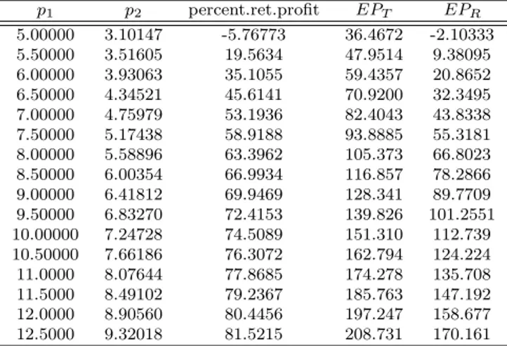
In case 2, when Q1 = Q2 = 13, positive profit for the retailer starts with
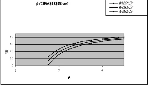
prices 5.50 and 3.516 for product 1 and 2 respectively and the corresponding percentage profit of the retailer is 19.5 and the total channel profit is 47.95. As prices increase both the total profit and the retailer‘s percentage share increase, reaching to about 80 percent share when the goods are sold about four times their cost. When tables E.9 to E.11 are compared, we see that the total profit increases substantially. Same observation also holds in comparison of the Tables E.12 to E.14, where Q1 = 20.
Case-6 corresponds to two way full substitution with partial credit and full returns. Hence both products are substituted with each other. In this case, we observe that coordination is possible for (Q1, Q2) values given by (20,20),
(20,27), (27,20), (27,27), all of which are above mean demand levels, which makes sense due to full substitution of both products. From Tables E.15 and E.18 we observe that the total profits and the share of the retailer are very close to each other with similar prices and slightly different s1, s2 values. When
these results are compared to the case with Q1 = 20, Q2 = 27, we note that for
Conclusion
In this study, a simple supply chain structure with a single retailer and a manufacturer, is considered for two perishable products which can be substituted for each other with fixed probabilities. The retailer is also allowed to return some products to the manufacturer according to the contract between the retailer and the manufacturer. The aim is to analyse the model so as to achieve channel coordination. By channel coordination, we refer to a case where the order quantity of the retailer is equal to the production quantity of a manufacturer that produces as well as sells the products. This means that the order quantities making the total expected channel profit maximum equals to the order quantity that makes the retailer‘s expected profit maximum as well. Using the model notations and assumptions, we first derive the expressions for the total expected channel profit, manufacturers expected profit and the retailers expected profit under general model parameters. We then investigated the special cases for channel coordination. These special cases are full returns with partial credit and no substitution; full returns with partial credit and one-way full substitution; one-way full substitution with no returns (only one product is substituted for other); full returns with full credit and one-way full substitution; two-way full substitution with no returns; full return with partial credit and way full substitution and full return with full credit and two-way full substitution. A similar study with a single product was given by
Pasternack [9], where it was found that channel coordination was not achieved with full returns and full credits. This is consistent with our result. We have found that channel coordination is not achieved for no returns cases. We have done the numerical studies with negative binomial demand distribution. From our results, we observed that the share of the retailer is substantially increased with two-way full substitution.
This study can be extended for multi products, multi-period , correlated demand and partial substitution as future research directions.
The calculation of the
EP
T
(Q
1
, Q
2
)
The derivation of the formula is based on considering the profit in several subcases as seen in Figure D.1. The cost of producing Q1 units of product 1
and Q2units of product 2, −c1Q1−c2Q2, is summed up with the profit obtained
by the integration of profit expressions over their respective regions as seen in Figure D.1 to obtain the formula, EPT(Q1, Q2) . The profit expressions in
each region is as follows:
πa = p1x+ p2y x ≤ Q1, y ≤ Q2 (a) πb = p2y+ p2ax+ Q1(p1−p2a) x ≥ Q1, y ≤ Q2, a(x − Q1) < Q2−y (b) πc= p1Q1+ p2Q2 x ≥ Q1, y ≤ Q2, a(x − Q1) > Q2−y (c) πd = p1Q1+ p2Q2 x ≥ Q1, y ≥ Q2 (d) πe = p1Q1+ p2Q2 x ≤ Q1, y ≥ Q2, Q1−x < b(y − Q2) (e) πf = p1x+ p1by+ Q2(p2−p1b) x ≤ Q1, y ≥ Q2, Q1−x > b(y − Q2) (f)
The same parts in πa, πb, πc, πd, πe and πf are grouped according to regions
in Figure D.1. As a result,
p1x in region (a ∪ f ) gives the following integral part of EPT(Q1, Q2): p1 Z Q1 0 x Z Q2+(Q1−x)b 0 dG(y)dF (x) = p1 Z Q1 0 xG(Q2+ (Q1 −x) b )dF (x) = (1) (1) can be extended by using integration by parts as follows:
p1Q1G(Q2)F (Q1) − p1 Z Q1 0 G(Q2+ (Q1−x) b )F (x)dx +p1(Q1+ bQ2) Z Q2+Q1b Q2 F(Q1+ b(Q2 −u))dG(u) −p1b Z Q2+Q1 b Q2 F(Q1+ b(Q2−u))udG(u) (2)
Similarly, p2y in region (a ∪ b) is symmetric to p1x.
p2 Z Q2 0 yF(Q1+ (Q2−y) a )dG(y) (3) (3) means; p2Q2G(Q2)F (Q1) − p2 Z Q2 0 F(Q1+ (Q2−x) a )G(x)dx +p2(Q2+ aQ1) Z Q1+Q2a Q1
G(Q2+ a(Q1−u))dF (u)
−p2a
Z Q1+Q2a
Q1
G(Q2+ a(Q1−u))udF (u) (4)
p1by in region (f ) gives the following integral part of EPT(Q1, Q2):
p1b Z Q2+Q1b Q2 y Z Q1+b(Q2−y) 0 dF(x)dG(y) = p1b Z Q2+Q1b Q2 yF(Q1+ b(Q2−y))dG(y) (5)
Similarly, p2ax in region (b) is symmetric to p1by.
p2a
Z Q1+Q2a
Q1
xG(Q2+ a(Q1 −x))dF (x) (6)
Q2(p2−p1b) in region (f ) gives the following integral part of EPT(Q1, Q2):
Q2(p2−p1b) Z Q2+Q1b Q2 F(Q1+ b(Q2−y))dG(y) = Q2(p2−p1b)[−F (Q1)G(Q2) + Z Q1 0 G(Q2+ (Q1−x) b )dF (x)] (7)
Similarly, Q1(p1−p2a) in region (b) is symmetric to Q2(p2−p1b). Q1(p1 −p2a) Z Q1+Q2a Q1 G(Q2+ a(Q1−x))dF (x) = Q1(p1−p2a)[−F (Q1)G(Q2) + Z Q2 0 F(Q1+ (Q2−y) a )dG(y)] (8)
p1Q1+ p2Q2 is in region (d ∪ e ∪ c), and each part is integrated seperately
as follows:
p1Q1+ p2Q2 in region (d) gives the following integral part.
(p1Q1+ p2Q2) Z ∞ Q1 Z ∞ Q2 dG(y)dF (x) = (p1Q1+ p2Q2)F (Q1)G(Q2) (9)
p1Q1+ p2Q2 in region (e) gives the following integral part.
(p1Q1+ p2Q2) Z ∞ Q1 Z ∞ Q2+(Q1−x)b dG(y)dF (x) = (p1Q1+ p2Q2) Z Q1 0 G(Q2+ (Q1−x) b )dF (x) = (p1Q1+ p2Q2)(F (Q1) − Z Q1 0 G(Q2+ (Q1 −x) b )dF (x))(10)
p1Q1+ p2Q2 in region (c) is symmetric to in region (e).
(p1Q1+ p2Q2)(G(Q2) − Z Q2 0 F(Q1+ (Q2−y) a )dG(y)) (11) The sum of (9), (10) and (11) gives the following integral part.
(p1Q1+ p2Q2)[1 + G(Q2)F (Q1) − Z Q2 0 F(Q1+ (Q2−y) a )dG(y) − Z Q1 0 G(Q2+ (Q1 −x) b )dF (x) (12)
EPT(Q1, Q2) is obtained by the sum of (2), (4), (5), (6), (7), (8), (12) and
The calculation of the
EP
R
(Q
1
, Q
2
)
The derivation of the formula is based on considering the profit in several subcases as seen in Figure D.2. The paid money to the manufacturer ,−d1Q1−
d2Q2, is summed up with the profit obtained by the integration of the profit expressions over their respective regions as seen in Figure D.2 to obtain the formula, EPR(Q1, Q2) . The profit expressions in each region is as follows:
x ≤(1 − R1)Q1, y ≤(1 − R2)Q2 πa = p1x+ p2y+ R1Q1s1+ R2Q2s2 (a) x ≤(1 − R1)Q1,(1 − R2)Q2 ≤y ≤ Q2 πb = p1x+ p2y+ R1Q1s1+ (Q2 −y)s2 (b) y ≥ Q2, Q1−(x + b(y − Q2)) > R1Q1 πc= p1x+ p1(b(y − Q2)) + R1Q1s1+ p2Q2 (c) y ≥ Q2, Q1−(x + b(y − Q2)) < R1Q1, x+ b(y − Q2) < Q1 πd = p2Q2+ p1(x + b(y − Q2)) + (Q1−x − b(y − Q2))s1 (d) 42
y ≤(1 − R2)Q2,(1 − R1)Q1 ≤x ≤ Q1 πe = p1x+ p2y+ R2Q2s2+ (Q1−x)s1 (e) (1 − R1)Q1 ≤x ≤ Q1,(1 − R2)Q2 ≤y ≤ Q2 πf = p1x+ p2y+ (Q1−x)s1+ (Q2 −y)s2 (f) x ≥ Q1, Q2−(y + a(x − Q1)) > R2Q2 πg = p2y+ p2(a(x − Q1)) + R2Q2s2+ p1Q1 (g) x ≥ Q1, Q2−(y + a(x − Q1)) < R2Q2, y+ a(x − Q1) < Q2 πh = p1Q1+ p2(y + a(x − Q1)) + (Q2−y − a(x − Q1))s2 (h) x ≥ Q1, y ≥ Q2 πi = p1Q1 + p2Q2 (i) y ≥ Q2, x+ b(y − Q2) < Q1, x < Q1 πj = p1Q1+ p2Q2 (j) x ≥ Q1, y+ a(x − Q1) < Q2, y < Q2 πk = p1Q1+ p2Q2 (k)
The same parts in πa, πb, πc, πd, πe, πf, πg, πh, πi, πj and πk are grouped
according to regions in Figure-D.2. As a result,
p1x in region a ∪ b ∪ e ∪ f gives the following integral part of EPR(Q1, Q2):
p1 Z Q1 0 x Z Q2 0 dG(y)dF (x) = p1G(Q2) Z Q1 0 xdF(x) = p1Q1F(Q1)G(Q2) − p1G(Q2) Z Q1 0 F(x)dx (1)
Similarly, p2y in region (a ∪ b ∪ e ∪ f ) is symmetric to p1x.
p2F(Q1) Z Q2 0 ydG(y) = p2Q2F(Q1)G(Q2) − p2F(Q1) Z Q2 0 G(y)dy (2)
R1Q1s1 in region (a ∪ b) gives the following integral part : Z Q2 0 x Z R1.Q1 0 R1Q1s1dF(x)dG(y) = R1Q1s1F(R1.Q1)G(Q2) (3)
Similarly, R2Q2s2 in region (a ∪ e) is symmetric to R1Q1s1.
R2Q2s2G(R2.Q2)F (Q1) (4)
(Q2−y)s2 in region (b ∪ f ) gives the following integral part :
Z Q2 R2.Q2 x Z Q1 0 dF(x)dG(y) = −R2Q2s2F(Q1)G(R2.Q2) + s2F(Q1) Z Q2 R2.Q2 G(y)dy (5)
(Q1−x)s1 in region (b ∪ f ) which is symmetric to (Q2−y)s2
−R1Q1s1G(Q2)F (R1.Q1) + s1G(Q2)
Z Q1
R1.Q1
F(x)dx (6)
p1Q1+ p2Q2 in region (i) gives the following integral part.
Z ∞ Q1
Z ∞ Q2
(p1Q1+ p2Q2)dG(y)dF (x) = (p1Q1+ p2Q2)G(Q2)F (Q1) (7)
The sum of (1),(2),(3),(4),(5),(6) and (7) gives the following integral part of EPR(Q1, Q2): p1Q1F(Q1)G(Q2) + F (Q1)[s2 Z Q2 R2.Q2 G(y)dy − p2 Z Q2 0 G(y)dy] +G(Q2)[s1 Z Q1 R1.Q1 F(x)dx − p1 Z Q1 0 F(x)dx] +(p1Q1+ p2Q2)G(Q2)F (Q1) (8)
p2Q2 in region (c ∪ d ∪ j) gives the following integral part.
Z ∞ Q2
Z Q1
0
p2Q2dF(x)dG(y) = p2Q2G(Q2)F (Q1) (9)
p1Q1 in region (j) gives the following integral part.
Z ∞ Q2 Z Q1 Q1−(b(y−Q2)) p1Q1dF(x)dG(y) = p1Q1G(Q2)F (Q1) − p1Q1 Z ∞ Q2 F(Q1−(b(y − Q2)))dG(y) (10)