Process Variation Aware Thread Mapping for Chip
Multiprocessors
S. Hong and S.H.K. Narayanan and M. Kandemir
Department of Computer Science and EnginneeringThe Pennsylvania State University {shhong, snarayan. kandemir}@cse.psu.edu
¨
O. ¨
Ozturk
Department of Computer Engineering Bilkent University
Abstract—With the increasing scaling of manufacturing
technol-ogy, process variation is a phenomenon that has become more prevalent. As a result, in the context of Chip Multiprocessors (CMPs) for example, it is possible that identically-designed processor cores on the chip have non-identical peak frequencies and power consumptions. To cope with such a design, each processor can be assumed to run at the frequency of the slowest processor, resulting in wasted computational capability. This paper considers an alternate approach and proposes an algorithm that intelligently maps (and remaps) computations onto available processors so that each processor runs at its peak frequency. In other words, by dynamically changing the thread-to-processor mapping at runtime, our approach allows each processor to maximize its performance, rather than simply using chip-wide lowest frequency amongst all cores and highest cache latency. Experimental evidence shows that, as compared to a process variation agnostic thread mapping strategy, our proposed scheme achieves as much as 29% improvement in overall execution latency, average improvement being 13% over the benchmarks tested. We also demonstrate in this paper that our savings are consistent across different processor counts, latency maps, and latency distributions.With the increasing scaling of manufacturing technology, process variation is a phenomenon that has become more prevalent. As a result, in the context of Chip Multiprocessors (CMPs) for example, it is possible that identically-designed processor cores on the chip have non-identical peak frequencies and power consumptions. To cope with such a design, each processor can be assumed to run at the frequency of the slowest processor, resulting in wasted computational capability. This paper considers an alternate approach and proposes an algorithm that intelligently maps (and remaps) computations onto available processors so that each processor runs at its peak frequency. In other words, by dynamically changing the thread-to-processor mapping at runtime, our approach allows each processor to maximize its performance, rather than simply using chip-wide lowest frequency amongst all cores and highest cache latency. Experimental evidence shows that, as compared to a process variation agnostic thread mapping strategy, our proposed scheme achieves as much as 29% improvement in overall execution latency, average improvement being 13% over the benchmarks tested. We also demonstrate in this paper that our savings are consistent across different processor counts, latency maps, and latency distributions.
I. INTRODUCTION
As processor design has become severely power and complex-ity limited, it is now generally accepted that multi-core architec-tures represent a promising alternative to conventional complex single core architectures. As a result, several manufacturers have dual core chips on the market (e.g., Intel’s dual core Montecito [3], the dual core AMD Athlon [2]), with more aggressive configurations being delivered or prototyped (e.g., Sun’s eight core Niagara [23], IBM’s Cell [5], Intel’s quad core Xeon [4], and Intel’s 80 core TeraFlop [1]). In addition to power and complexity advantages, chip multiprocessors (CMPs) are also preferable from the reliability and thread level parallelism perspectives.
In addition to well known issues of concurrent programming, reliability and power management in CMPs [27], [10], there is a newly emerging and significant obstacle as we move toward future CMPs with a large number of cores: process variation [15], [26], [29], [12], [17]. In deep sub-micron design technology, it is becoming increasingly difficult to control critical transistor parameters such as gate-oxide thickness, channel length, and dopant concentrations. As a result, these parameters may have different values than nominal, and this may, in turn, lead to both power and timing variability across identically-designed
components of a CMP. One option to cope with process variation is to operate under the worst case scenario. In this operation mode, worst possible latencies are assumed for affected hardware components. However, this option becomes less attractive as technology scales downward because the difference between the worst case and average case increases dramatically [30].
The main contribution of this paper is process variation aware thread mapping support for CMPs. Focusing on a CMP architecture with latency variations across identically-designed processor cores and across identically-designed L1 caches, this paper proposes and experimentally evaluates a process variation aware thread remapping algorithm that allows all the processors to operate at their individual peak frequency. This algorithm makes use of an important characteristic of the application domain we target, namely, data intensive codes, where a series of loop nests operate on large data structures and these loops iterate many times during execution.
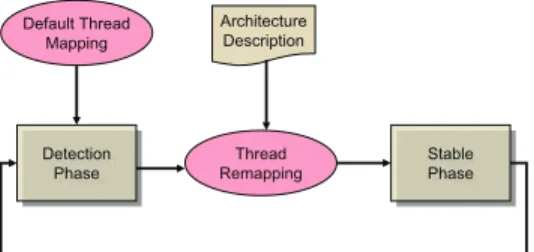
The proposed thread mapping phase algorithm is dynamic (i.e., applied at runtime) and, has two alternating phases, namely detection phase and stable phase that are separated by a remap-ping step, as illustrated in Figure 1. In the detection phase, the variations across the execution latencies of different threads are captured by executing one iteration of the loop nest being optimized. Note that these latency variations can originate from inherent thread characteristics (e.g., one thread may have lower cache miss rate than another) or from process variation, or from a combination of both. In any case, one can take advantage of these variations by remapping the parallel threads differently for the remaining portion of the loop execution. This remapped execution constitutes the stable portion of the proposed approach. Note that the detection and stable phases can be repeated multiple times for the same loop nest to accurately capture the loop behavior at runtime, and to better adapt application execution.
Our experimental evaluation clearly shows that the proposed scheduling scheme is very effective in practice and improves performance by as much as 29% over a standard thread mapping scheme which is process variation agnostic. We also found that the average improvement brought by our thread mapping scheme is about 13%. Finally, we study the sensitivity of our approach to different values of processor frequency and cache latency, as well as the number of remappings performed and the number of processors in the CMP.
The remainder of this paper is structured as follows. Section II discusses the related work. Section III briefly explains the phenomenon of process variation. Section IV introduces the applications that are targeted in this work, and Section V gives the details of our thread mapping algorithm. Section VI presents an example of the mapping algorithm. Section VII presents an experimental evaluation of the proposed mapping approach. Finally, we conclude with a summary in Section VIII.
II. RELATEDWORK
There exist prior publications on qualifying and addressing the impact of process variation. Several recent studies illustrate the impact of the process variation on performance [15], [26], [29], [12], [17]. A statistical design methodology to improve benefits from a design that considers frequency binning is pro-posed in [11]. An analytical modeling approach [16], based
978-3-9810801-5-5/DATE09 © 2009 EDAA
Detection Phase Detection Phase Detection Phase Thread
Remapping StablePhaseStablePhase Stable Phase Architecture Description Default Thread Mapping
Fig. 1. The high level view of our approach. Dynamic remapping takes place in a cycle consisting of a detection phase and a stable phase separated by a remapping step. The detection phase takes as input the default or previous thread to processor mapping. The remapping step uses the architectural description and the output of the detection phase.
on understanding different power and variation sensitivities, is developed to obtain the power reduction benefits. A method of addressing within-die process variation in the routing of FPGAs is presented in [25]. Past work also proposes a process-tolerant cache architecture [9] and studies process variation aware cache leakage management [22]. An analytical approach for ensuring timing reliability while meeting the appropriate performance and power demands in the existence of process variation is proposed in [19]. Process variation aware parallelization strategies for embedded MPSoCs to lower power consumption are described in [30]. In that work, it is mentioned that dynamic mapping of applications based on run-time traces can be very important.
Our work is different from these prior studies because most of them do not focus on performance. Specifically, [15], [26], [29], [12], [17] discuss the impact of process variation on chips. In comparison, [11] and [9] focus on profit and yield, respectively. Power improvement is studied in [22], [19], [16], and FPGA is studied in [25]. In addition, most of the above papers are not targeted at chip multiprocessors. [30] proposes a solution to tackle the energy-delay product increase in embedded MPSoCs; how-ever, the solution proposed essentially performs a static mapping of applications. In contrast, our work focuses on dynamic thread remapping for migrating the impact of process variation.
III. PROCESSVARIATION
Variations in the manufacturing technology, such as deposition depths, impurity concentration densities, limited resolution of photo-lithography and oxidation thickness are the main cause of process variation. Furthermore, process variations are also caused by the external environment, such as the processing temperature and voltage. Process variations can be separated into two categories, die-to-die and within-die fluctuations [15], [13], [12]. Die-to-die fluctuations affect the different circuit parts differently, while within-die fluctuations affect all parts equally.
The basic characteristics of an IC circuit, such as device dimension W/L, transistor current and threshold voltage, may be affected by process variations. For example, the standby current spread in circuits is caused by the variations in channel length. As a result, both the mean value and distribution of the circuit frequency will be impacted. Besides, other characteristics of the chip, such as energy dissipation, reliability and lifetime, can also be influenced negatively. Thus, the circuit may not work as a designer would expect it to.
With the increasing scaling of the multiprocessors, process variations have become an important obstacle in achieving high circuit performance. For instance, identically designed processors in the CMPs may have different (lower) peak frequencies [30]. As mentioned earlier, it is possible to operate under process variations by assuming the worst possible latencies for hardware components that are affected by process variation. Clearly, this option is becoming less attractive with the scaling of technology.
L2 Cache P1 L1 P1 L1 P1 L1 P1 L1 P1 L1 P1 L1 P1 L1 P1 L1
Fig. 2. A CMP architecture composed of 8 processors. Each processor has a private L1 cache and is connected to a shared L2 cache.
Algorithm 1 Sample Benchmark ()
1: for (i= 1; i ≤ Q; i + +) do 2: !$omp parallel 3: for (j= 1; j ≤ N; j + +) do 4: . . . 5: end for 6: barrier() 7: end for
IV. TARGETAPPLICATIONTEMPLATE
The applications in consideration consist of loop based compu-tations manipulating arrays. These applications typically consist of an outer loop within which significant computation takes place, as outlined in Algorithm 1. The computation within the outer loop, which consists of Q iterations, is parallelized according to the architecture that it is run upon which in this work is a CMP as shown in Figure 2.
Inherent differences in thread behaviors with respect to control branches and cache accesses result in a difference in the amount of computation that is performed by each thread. In addition to the differences between the threads, the behavior of a given thread itself may vary as well during the course of their execution. There-fore, the execution of a thread can be thought of as happening in stages (epochs). This allows the characterization of the application according to whether there are differences between the stages of execution or not.
The application parallelization technique that is used is pre-sented in [18], though the selection of the parallelization strategy is orthogonal to the main focus of our paper. The parallelized program uses synchronization, to avoid race conditions and to ensure the coherence of the data values. Barriers are a common synchronization operation in programs with parallel loops. A thread is forced to wait at the barrier until all other threads reach the barrier at which point all the threads are released.
Our experimental evaluations use parallel programs with the barrier supported by OpenMP. The programs use an OpenMP compiler directive, !$omp parallel, to parallelize an inner loop, which is inside an outer loop as shown in Algorithm 1. The barrier guarantees that each thread is done in the inner loop before they start the next iteration of the outer loop.
V. DETAILS OF THEALGORITHM
Under the proposed dynamic remapping approach, the execu-tion of the applicaexecu-tion occurs at the granularity of an epoch, which consists of a detection phase and a stable phase, separated by a
thread remapping step.
Detection Phase. In the detection phase the threads of the parallelized application are mapped to processors using a default mapping and are run for one iteration of the outer loop of the thread. In the case of the first epoch the default mapping is random. The number of processor cycles taken to execute each thread are measured during this initial run of the threads. In addition to the processor cycles, the number of cache accesses
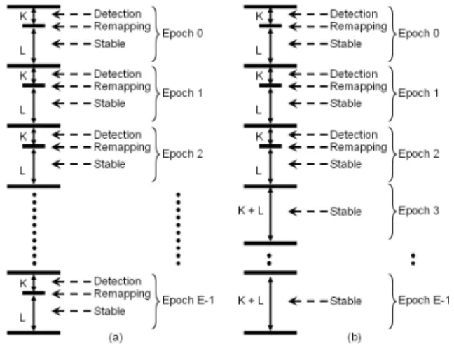
Fig. 3. The execution of the threads takes place at the granularity of an epoch. It is assumed that that the value of K is 1. (a) A varying application may be remapped at every epoch (b) A uniform application is not remapped after the first three epochs.
TABLE I
THE ASSUMEDCPUFREQUENCIES AND THEL1CACHE LATENCIES.
CPU Frequency L1 Latency GHz Cycles
1 1.1 2
2 1.1 3
3 1 2
4 1 3
are also measured. These measurements can easily be performed using performance counters available on modern processors. In our framework, the total load of each thread is expressed by the tuple{processor cycles, cache cycles}; i.e., the cycles taken by the processor and the cycles spent in accessing the L1 cache. The threads are then ranked in decreasing order of their load. As there are two measures to sort the threads by, radix sort is used to sort the threads. The approach then enters the remapping step.
Remapping Step. In the remapping step, the threads which have just been sorted are mapped to the processors. The thread with the most load is assigned to the processor-cache pair with the fastest frequency and cache latency combination. After that, the thread with the second highest load is assigned to the processor-cache pair with the second fastest frequency and processor-cache latency combination. This strategy is followed until all the threads are scheduled in the order of decreasing load; that is, in the order of decreasing frequency and cache latency combination speed.
Stable Phase. The new mapping is then used to run the threads on the processors for a fixed number of iterations called the stable phase. The end of the stable phase concludes an epoch.
Initially, each application is executed for three epochs. The default mapping for the second epoch’s detection phase is the mapping used in the stable phase of the first epoch. Similarly, the default mapping for the third epoch’s detection phase is the mapping used in the stable phase of the second epoch. At the end of the third epoch, the application is characterized based on whether the threads change their behavior from epoch to epoch. The characterization is used to decide whether the threads will undergo further remapping or not.
The behavioral information of the threads is maintained in a history table that contains the rank of each thread for the first three epochs. Each entry in the table keeps track of ranking of a particular thread amongst all threads at the end of that detection phase of that epoch. This allows the application in question to be classified as being either uniform or varying (at the end of the third epoch). If the ranking of all the threads remains the same from epoch to epoch, then the application said to be uniform. A uniform application is not remapped further and the threads continue to completion. If the ranking of the threads changes, the
TABLE II
THE INSTRUCTION CYCLES,CACHE ACCESS CYCLES CAPTURED BY
THE DETECTION PHASE ARE SHOWN IN COLUMNS2AND3
RESPECTIVELY. THE RANKING OF THE THREADS IS SHOWN IN
COLUMN4. THE NEW MAPPING OF THREADS TO PROCESSORS IS
SHOWN COLUMN5.
Thread Processor L1 Access Ranking Processor Cycles Cycles Assignment
1 100 15 4 4
2 120 12 2 2
3 100 18 3 3
4 130 12 1 1
TABLE III
THE HISTORY TABLE OF THE
RANK OF THE THREAD AFTER THE DETECTION PHASE IN
THE FIRST THREE CYCLES. AS
THE RANKS OF ALL THE
THREADS REMAIN THE SAME,
THE CORRESPONDING APPLICATION IS CONSIDERED TO BE UNIFORM. Thread Id Cycle 1 2 3 1 4 4 4 2 2 2 2 3 3 3 3 4 1 1 1 TABLE IV THE ASSUMED HISTORY
TABLE OF THE RANK OF THE THREAD AFTER THE DETECTION PHASE IN THE
FIRST THREE CYCLES. AS THE
RANKS OF THE THREADS VARY FROM CYCLE TO
CYCLE,THE CORRESPONDING
APPLICATION IS CONSIDERED TO BE VARYING. Thread Id Cycle 1 2 3 1 4 4 2 2 2 2 4 3 3 1 3 4 1 3 1
application is classified as varying, and further remapping(s) can be performed. That is, the threads are run epoch by epoch with a possible remapping occurring in each epoch. Figure 3, illustrates the epochwise execution of a varying application as well as a uniform application.
VI. EXAMPLE
This section presents an example application of the thread mapping algorithm outlined in Section V. The architecture is assumed to be a CMP made up of 4 processors, each with a private L1 data cache. Table I gives the operating frequency of the processors in the CMP as well as the latency of their L1 caches. Let us also assume that the outer loop in the example benchmark (see Algorithm 1) consists of 200 iterations (that is, Q = 200) and is parallelized to consist of 4 threads of 50 iterations each. Let an epoch consist of4 iterations : 1 iteration for the detection phase and3 iterations for the stable phase. In the detection phase of the first epoch, the processor cycles and the L1 cache access cycles are measured. Their values are assumed to be as shown in the second and the third columns of Table II, respectively.
It is clear that the processor cycles are larger than the cache access cycles. Therefore, the radix sort algorithm that is used to sort (in decreasing order) the threads treats the processor cycle value as the primary parameter and the L1 access cycles as the secondary parameter. The rank of each thread at the end of the first detection phase is shown in the fourth column of Table II. The mapping at the end of the detection phase of the first epoch is shown in column five of Table II. After that, the threads are run for two further epochs, to classify the benchmark as either uniform or varying. The rank of the threads at the end of each the detection of each epoch is shown in Table III (called the history table). As the rank of each thread remains the same across the cycles, the benchmark is classified as uniform and the threads run to completion without any further dynamic detection or remapping. In order to illustrate a different scenario, let us assume the rank of the threads in the three epochs are different, as shown in Table IV. In this case, the benchmark is classified as varying, and executed at the granularity of an epoch (detection phase, remapping step, stable phase) until completion.
VII. EXPERIMENTALEVALUATION
In this section, we describe the simulation strategy used to eval-uate our approach and compare the results obtained against those
TABLE V
THE DETAILS OF THENPB3.2-OMPBENCHMARKS USED IN OUR
EXPERIMENTS. THE EXECUTION CYCLES HAVE BEEN GENERATED BY
RUNNING THE OUTER LOOP OF THE BENCHMARKS FOR100
ITERATIONS.
Program Brief Execution
Name Explanation Cycles (M) FT Fast Fourier Transform 174018 UA Solver for a stylized 1447
heat transfer problem
BT CFD application 25327 SP CFD application 25328 MG MultiGrid method 33151 LU Solver for a seven-block-diagonal 18370 system LU-HP Hyper-plane 18092 version of LU TABLE VI
THE PROCESSOR FREQUENCIES AND CACHE ACCESS LATENCIES
USED IN THE EXPERIMENTS.
CPU Frequency L1 Latency GHz Cycles
1,2 1.1 2
3,4 1.1 3
5,6 1 2
7,8 1 3
obtained using alternate thread mapping approaches. Finally, we examine the sensitivity of our approach to parameters such as the number of remappings and the number of processors in the architecture.
Our simulation methodology consists of two steps. First, we determine the cycle-wise load of each thread by simulating it on our CMP architecture. Following that, we feed the values ob-tained from the simulation to our implementation of the dynamic thread remapping scheme to obtain the execution times of each benchmark. The architecture used in the experiments is an 8-processor CMP (see Figure 2). Each 8-processor is connected to an 8 KB private L1 cache and a shared L2 cache. The processors are based on the UltraSPARC III architecture [6].
The architecture in consideration was simulated using Simics [8]. Simics is a full system simulation platform that supports Unix executables for various processors, such as the UltraSPARC III. We created configuration files to implement a CMP with 8 processors. We also modified the g-cache system in Simics to gather sharing characteristics of the last-level cache [20].
The seven benchmark application codes used in this work are from the NPB Suite [21]. In order to determine the cycle-wise load of the application threads, they were run on the Simics based implementation of the CMP described earlier. In this particular implementation, all the processors run at 1 GHz and the cache access latency is 3 cycles (i.e., there is no process variation). Run-ning the threads on these processors allows the processor cycles and the number of cache accesses to be measured. Note that, by measuring the number of cycles taken to execute the threads and not the time taken to execute them, the frequency at which each processor is functioning does not affect the calculation of the computation load of the threads. The details of the benchmarks are given in Table V. The benchmarks are parallelized by the use of OpenMP [7], [18] directives. The first column of Table V gives the benchmark name and the second column describes it briefly. The third column shows the execution cycles (in millions) when no specific optimization targeting process variations is applied.
The detection phase, remapping step and stable phase of our proposed approach are implemented in C++. They are given as input the architectural details and the cycle-wise load of the threads. In order to simulate process variation, the processors in the CMP, whose information is provided as input to the C++ implementation, are configured to operate at different frequencies.
0.65 0.7 0.75 0.8 0.85 0.9 0.95 1 FT UA BT SP MG LU LU-HP
Normalized Execution Time
Random Ideal Dynamic Random Dynamic Best
Fig. 4. The normalized execution time of the ideal, random, dynamic
random and dynamic best schemes when applied to the seven benchmark
applications using the processor frequencies and cache latencies shown in Table VI. The execution times are normalized to the process variation agnostic approach. 0% 10% 20% 30% 40% 50% 60% 70% 80% 90% 100% FT UA BT SP MG LU LU-HP
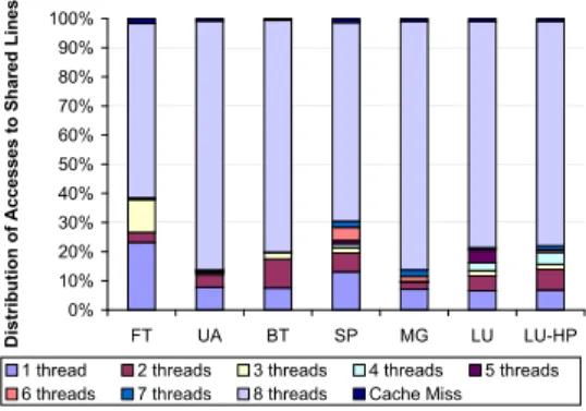
Distribution of Accesses to Shared Lines
1 thread 2 threads 3 threads 4 threads 5 threads
6 threads 7 threads 8 threads Cache Miss
Fig. 5. Distribution of accesses to caches lines according to the number of threads that share that line. The graph shows that a large majority of cache lines are shared by all the threads.
Further, the caches are configured to have different access laten-cies. The assumed processor frequencies and L1 cache latencies are shown in Table VI. For example, processors 1 and 2 operate at 1.1 GHz each and the access latency of their L1 cache is 2 cycles. The implementations of the detection phase, remapping step and stable phase are then used to simulate the running of the benchmark applications to obtain the total execution times. A. Ideal and Random Schemes
In order to study the effectiveness of our remapping algorithm, we measured the performance results of the proposed dynamic remapping approach (called dynamic random 1 as well) against
two extreme schemes called ideal and random and a variation of the proposed approach called dynamic best. In the ideal scheme, the computation load for each thread is computed at the granu-larity of an iteration of the outer loop. Then, for each iteration, a new ranking of the threads is generated. The remapping step is given as the input the ranking of threads and the frequencies of the processors and cache access latencies. This allows the remapping step to create the ideal mapping of threads to the processors at the granularity of an iteration. The running of the threads is then simulated using the ideal mapping and the execution time is measured. Note that, this ideal scheme is difficult to implement in practice due to extremely high re-mapping costs (as mapping can potentially change at every iteration). In our results with this scheme, we omit its overheads to quantify the best theoretical performance.
For the random scheme, the mapping unit randomly maps a thread to processors. The running of the threads is then simulated using this mapping and the execution time is measured. The dynamic best scheme is exactly the same as our dynamic random scheme, except that the default (initial) mapping of threads to
1The reason that we use the word ”random” is to is that the initial mapping is
TABLE VII
THREE DIFFERENT SCENARIOS OF
PROCESSOR DISTRIBUTIONS IN THE
FREQUENCY RANGE1 GHZ TO1.4 GHZ.
EACH ENTRY DESCRIBES HOW MANY
PROCESSORS OPERATE AT A PARTICULAR FREQUENCY FOR A PARTICULAR
SCENARIO. Frequency (GHz) 1.0 1.1 1.2 1.3 1.4 Scenario A 1 6 1 0 0 Scenario B 1 3 3 1 0 Scenario C 1 2 2 2 1 TABLE VIII
THE POSSIBLE FREQUENCIES THAT
PROCESSORS OPERATE AT. NOTE THAT,
ALTHOUGH THE DIFFERENCE BETWEEN THE HIGHEST AND LOWEST FREQUENCIES REMAINS THE SAME IN BOTH RANGES,I.E. 0.5 GHZ;THE RELATIVE DIFFERENCE BETWEEN THE PROCESSORS IS LARGER IN
THELowerRANGE AND SMALLER IN THE
HigherRANGE. Name Frequency Range Lower 0.5 0.6 0.7 0.8 0.9 Higher 2.0 2.1 2.3 2.4 2.5
TABLE IX
THREE DIFFERENT SCENARIOS OF CACHE
DISTRIBUTIONS ACROSS THE DIFFERENT
LATENCIES(1, 2OR3CYCLES). EACH
ENTRY DESCRIBES HOW MANY CACHES HAVE A PARTICULAR ACCESS LATENCY
FOR A PARTICULAR DISTRIBUTION TYPE.
Cache Access Latency
1 2 3 Type 1 0 4 4 Type 2 1 6 1 Type 3 2 4 2 0.65 0.7 0.75 0.8 0.85 0.9 0.95 1 FT UA BT SP MG LU LU-HP
Normalized Execution Time
Scenario A Scenario B Scenario C
Fig. 6. The normalized execution time of the processor distribution scenarios using the dynamic remapping approach. The execution times are normalized to the agnostic ap-proach. 0.65 0.7 0.75 0.8 0.85 0.9 0.95 1 FT UA BT SP MG LU LU-HP
Normalized Execution Time
Scenario A Scenario B Scenario C
Fig. 7. The normalized execution time of the processor frequency scenarios shown in Table VII with the Lower frequency range described in Table VIII using the dynamic remapping approach. The execution times are normalized to the worst case frequency execution time.
0.65 0.7 0.75 0.8 0.85 0.9 0.95 1 FT UA BT SP MG LU LU-HP
Normalized Execution Time
Scenario A Scenario B Scenario C
Fig. 8. The normalized execution time of the processor distribution scenarios shown in Table VII with the Higher frequency range described in Table VIII using the dynamic remapping approach. The execution times are normalized to the worst case frequency exe-cution time.
processors is more careful than the random scheme and considers process variations.
B. Results
Figure 4 shows the execution times of the ideal, random, dynamic random and dynamic best schemes for the seven bench-marks. The execution times are normalized to those of the process variation agnostic approach in which all the processors operate at the frequency of the slowest processor. It can be seen that the performance of the ideal scheme is the best across all the benchmarks. The performance of the proposed dynamic remapping scheme is poorer than the ideal scheme across all the benchmarks, but better than the random scheme. The execution times of the dynamic random and dynamic best schemes are almost identical, meaning that our approach is not very sensitive to the initial mapping of used and adapts very quickly.
Overall, the proposed approach saves an average of 5.84% execution time over the worst case frequency scheme and the ideal mapping scheme saves 7.36% on average. On the other hand, the random scheme saves3.57% execution time, which is half of the ideal scheme. This means that it does not make much sense to have a process variation aware scheme without using a form of dynamic remapping.
An important consideration is the overhead of remapping itself on the performance of the proposed approach. Remapping threads across processors could potentially lead to increased misses in the L1 cache. Figure 5 gives the L2 cache access distributions of our seven benchmarks on an eight-CPU CMP without process variations. We can observe that a significant fraction of total accesses, about77% on the average, are to cache lines that are shared by 8 threads. Therefore, when a remapping occurs, a thread can expect, most of the time, that the L1 cache of the processor that is mapped to will contain required data in about 77% of its lines. Therefore, the overhead of remapping a thread is in fetching the remaining portion of cache lines from the L2 cache into the L1 cache. On average, this can be computed as : (100 − 76.94) ∗ L1 Cache size ∗ L2 access latency, and is already included in our results.
C. Sensitivity Experiments
We now present the results of sensitivity experiments using the dynamic remapping approach (dynamic random). The first experiment is to vary the number of processors operating at the different frequencies. Table VII shows the three processor distributions in the frequency range 1 GHz to 1.4 GHz. Each scenario has a different number of processors operating at a particular frequency. The distribution of processors follows the Normal Distribution, which is expressed as :
X∼ N(μ, σ2),
where X is the process variation distribution, i.e., a processor frequency distribution, μ is the mean of the distribution, and σ is the standard deviation of the distribution. The detailed distribution model is provided in [14], [13], [24].
Figure 6 shows the performance of the different frequency distribution scenarios under the same cache access latency distri-bution. On average, the ”Scenario A”, ”Scenario B” and ”Scenario C” experiments reduce the execution time by9.70%, 11.78% and 13.25% respectively compared with the agnostic approach.
Similar to the variations for the processors, the access latency for an L1 cache is determined using the Normal Distribution as well. Table IX presents cache distributions across different access latencies. Figure 9 presents the execution times for the different cache distributions and the processor distribution Scenario B explained in Table VII.
Next, to check the sensitivity of the results obtained to the frequency range of the processors, the range of frequencies that the processors operate at is varied. Table VIII gives the two new sets of ranges of frequencies that the processors can operate at. The difference between the highest and lowest frequencies in both ranges is 0.5 GHz. This implies that the relative difference between the highest and lowest frequencies is larger in the Lower frequency range and smaller in the Higher frequency range.
Figure 7 shows the performance results for the Lower frequency range with the processor distributions shown in Table VII. Figure 8 shows the performance results for the Higher frequency range with the processor distributions shown in Table VII. By compar-ing the columns across the Figures 7, 6 and 8, we can observe
0.65 0.7 0.75 0.8 0.85 0.9 0.95 1 FT UA BT SP MG LU LU-HP
Normalized Execution Time
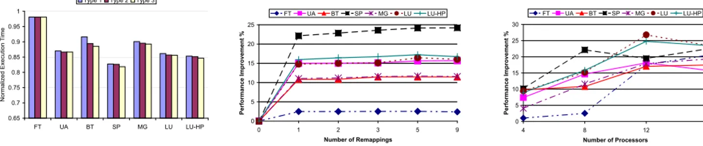
Type 1 Type 2 Type 3
Fig. 9. The normalized execution time of the different cache distributions using the dynamic remapping approach. The execution times are normalized to the agnostic ap-proach. 0 5 10 15 20 25 0 1 2 3 5 9 Number of Remappings Performance Improvement % FT UA BT SP MG LU LU-HP
Fig. 10. The normalized performance im-provement for different numbers of remap-pings using the dynamic remapping approach.
0 5 10 15 20 25 30 4 8 12 16 Number of Processors Performance Improvement % FT UA BT SP MG LU LU-HP
Fig. 11. The normalized performance im-provement for different numbers of proces-sors using the dynamic remapping approach. that the range that has a higher relative difference between the
lowest and highest frequency has more pronounced benefits. Next,we evaluate the impact of the number of dynamic remap-ping occurrences on the performance. The number of dynamic remappings is related to the number of instructions in the thread by the formula:
instruction count := remapping count
∗ detection phase size
In order to implement this experiment, the size of the detection phases in each thread is changed and the computation load per-cycle for each thread is recalculated. Figure 10 shows the benefits of increasing the number of remappings. We can see that for the benchmarks considered, the most significant benefit of remapping comes from performing the remapping once. The change in benefits for further remappings is not as significant. This is perhaps because, the benchmarks in consideration are mostly uniform and not varying.
Lastly, the sensitivity of the remapping approach to the number of processors in the architecture in consideration is examined. In order to implement this experiment, we parallelized the ap-plications such that the number of threads in the application is equal to the number of processors in the architecture. Following that, we used the dynamic mapping approach to simulate the running of the threads on the processors. Figure 11 presents the benefits of the dynamic remapping approach when the number of processors in the architecture varies. It should be noted that the benefits for a particular architecture are presented with respect to the worst case frequency result on that architecture. It can be seen that, overall, the benchmarks show greater benefits with an increase in the number of processors due to further opportunities for remapping. There are however, a few exceptions when the increase in processors results in a relative loss of benefits.
VIII. CONCLUSION
Process variation in CMPs leads to processors in the CMP operating at separate peak frequencies. This paper proposed and evaluated a dynamic thread remapping scheme that intelligently maps the threads of a parallel application to the different pro-cessors in the CMP. The remapping scheme operates in two alternating phases, remapping and stable and allows processors in a CMP to operate at their individual frequencies. The dynamic mapping approach maps the threads to the processors in the CMP based on the workload of the threads and the frequency of the processors. We studied the performance benefits offered by the remapping scheme on an 8 processor CMP. We found that, in comparison to a process variation agnostic scheme, the proposed scheme brings about a 29% improvement in overall execution latency, with the average improvement being 13% across all the benchmarks studied. Our results also showed that the improvement in execution latency increased in general with an increase in the number of processors in the CMP.
ACKNOWLEDGMENT
This research is supported in part by NSF Grants 0811687, 0720645, 0720749, and 0702519. REFERENCES [1] http://techresearch.intel.com/articles/Tera-Scale/1449.htm. [2] http://www.amd.com/us-en/Processors/ProductInformation/. [3] http://www.intel.com/pressroom/kits/itanium2/. [4] http://www.intel.com/products/processor/xeon5000/. [5] http://www.research.ibm.com/cell/.
[6] An Overview of UltraSPARC TM III Cu UltraSPARC III Moves to Copper
Technology Version 1.1, 2003.
[7] OpenMP Application Program Interface Version 2.5 Public Draft, 2004. [8] Simics User Guide for Unix 2.2.12, 2005.
[9] A. Agarwal, et al., “A process-tolerant cache architecture for improved yield in nanoscale technologies,” TVLSI, vol. 13, no. 1, pp. 27–38, Jan. 2005. [10] V. Agarwal, et al., “Clock rate versus ipc: the end of the road for conventional
microarchitectures,” in ISCA, 2000, pp. 248–259.
[11] D. Animesh, et al., “Speed binning aware design methodology to improve profit under parameter variations,” ASPDAC, pp. 6 pp.–, 24-27 Jan. 2006. [12] S. Borkar, et al., “Parameter variations and impact on circuits and
microar-chitecture,” DAC, pp. 338–342, 2-6 June 2003.
[13] K. Bowman, et al., “Impact of die-to-die and within-die parameter fluctua-tions on the maximum clock frequency distribution for gigascale integration,”
Solid-State Circuits, IEEE Journal of, vol. 37, no. 2, pp. 183–190, Feb 2002.
[14] K. Bowman, et al., “Maximum clock frequency distribution model with practical vlsi design considerations,” ICICDT, pp. 183–191, 2004.
[15] K. A. Bowman, et al., “Impact of die-to-die and within-die parameter vari-ations on the throughput distribution of multi-core processors,” in ISLPED, 2007, pp. 50–55.
[16] S. M. Burns,et al. “Comparative analysis of conventional and statistical design techniques,” in DAC, 2007, pp. 238–243.
[17] Y. Cao and L. T. Clark, “Mapping statistical process variations toward circuit performance variability: an analytical modeling approach,” in DAC, 2005, pp. 658–663.
[18] L. Chun, et al., “Exploiting barriers to optimize power consumption of cmps,” IPDPS, pp. 5a–5a, 04-08 April 2005.
[19] J. Donald and M. Martonosi, “Power efficiency for variation-tolerant multi-core processors,” in ISLPED, 2006, pp. 304–309.
[20] A. Jaleel, et al., “Last level cache (llc) performance of data mining workloads on a cmp - a case study of parallel bioinformatics workloads,” HPCA, pp. 88–98, 11-15 Feb. 2006.
[21] H. Jin, et al., The OpenMP Implementation of NAS Parallel Benchmarks
and Its Performance, October 1999.
[22] M. Ke and J. Russ, “Process variation aware cache leakage management,”
ISLPED, pp. 262–267, 4-6 Oct. 2006.
[23] P. Kongetira, et al., “Niagara: A 32-way multithreaded sparc processor,”
IEEE Micro, vol. 25, no. 2, pp. 21–29, 2005.
[24] H. Masuda, et al., “Challenge: variability characterization and modeling for 65- to 90-nm processes,” Custom Integrated Circuits Conference, 2005.
Proceedings of the IEEE 2005, pp. 593–599, 18-21 Sept. 2005.
[25] Y. Matsumoto, et al., “Performance and yield enhancement of fpgas with within-die variation using multiple configurations,” in FPGA, 2007, pp. 169– 177.
[26] S. Nassif, “Modeling and analysis of manufacturing variations,” Custom
Integrated Circuits, 2001, IEEE Conference on., pp. 223–228, 2001.
[27] B. Nayfeh and K. Olukotun, “A single-chip multiprocessor,” Computer, vol. 30, no. 9, pp. 79–85, Sep 1997.
[28] O. Ozturk, et al., “Compiler-directed variable latency aware spm manage-ment to cope with timing problems,” in CGO, 2007, pp. 232–243. [29] S. Samaan, “The impact of device parameter variations on the frequency
and performance of vlsi chips,” ICCAD, pp. 343–346, 7-11 Nov. 2004. [30] S. Srinivasan, et al., “Process variation aware parallelization strategies for