Linear MMSE-optimal turbo equalization using context trees

Linear MMSE-Optimal Turbo Equalization

Using Context Trees

Kyeongyeon Kim, Member, IEEE, Nargiz Kalantarova, Suleyman Serdar Kozat, Senior Member, IEEE, and

Andrew C. Singer, Fellow, IEEE

Abstract—Formulations of the turbo equalization approach to

iterative equalization and decoding vary greatly when channel knowledge is either partially or completely unknown. Maximum aposteriori probability (MAP) and minimum mean-square error (MMSE) approaches leverage channel knowledge to make explicit use of soft information (priors over the transmitted data bits) in a manner that is distinctly nonlinear, appearing either in a trellis formulation (MAP) or inside an inverted matrix (MMSE). To date, nearly all adaptive turbo equalization methods either estimate the channel or use a direct adaptation equalizer in which estimates of the transmitted data are formed from an expressly linear function of the received data and soft information, with this latter formulation being most common. We study a class of direct adaptation turbo equalizers that are both adaptive and nonlinear functions of the soft information from the decoder. We introduce piecewise linear models based on context trees that can adaptively approximate the nonlinear dependence of the equalizer on the soft information such that it can choose both the partition regions as well as the locally linear equalizer coefficients in each region independently, with computational complexity that remains of the order of a traditional direct adaptive linear equalizer. This approach is guaranteed to asymptotically achieve the performance of the best piecewise linear equalizer, and we quantify the MSE performance of the resulting algorithm and the convergence of its MSE to that of the linear minimum MSE estimator as the depth of the context tree and the data length increase.

Index Terms—Context tree, decision feedback, nonlinear

equal-ization, piecewise linear, turbo equalization. I. INTRODUCTION

I

TERATIVE equalization and decoding methods, or so-called turbo equalization [1]–[3], have become increas-ingly popular methods for leveraging the power of forward error correction to enhance the performance of digital commu-nication systems in which intersymbol interference or multiple access interference are present. Given full channel knowledge,

Manuscript received February 11, 2012; revised September 14, 2012 and Feb-ruary 19, 2013; accepted FebFeb-ruary 25, 2013. Date of publication April 04, 2013; date of current version May 20, 2013. The associate editor coordinating the re-view of this manuscript and approving it for publication was Prof. Xiao-Ping Zhang.

K. Kim is with Samsung Electronics, Yongin-si, Gyeonggi-do 446-712, Korea (e-mail: adrianakky@gmail.com).

N. Kalantarova is with the Electrical Engineering Department, Koc Univer-sity, Istanbul 34450, Turkey (e-mail: nkalantarova@ku.edu.tr).

S. S. Kozat is with the Electrical Engineering Department, Bilkent University, Ankara 06800, Turkey (e-mail: kozat@ee.bilkent.edu.tr).

A. C. Singer is with the Electrical and Computer Engineering Department at University of Illinois at Urbana-Champaign, Urbana, IL 61801, USA (e-mail: acsinger@illinois.edu).

Color versions of one or more of the figures in this paper are available online at http://ieeexplore.ieee.org.

Digital Object Identifier 10.1109/TSP.2013.2256899

maximum a posteriori probability (MAP) equalization and de-coding give rise to an elegant manner in which the equalization and decoding problems can be (approximately) jointly resolved [1]. For large signal constellations or when the channel has a large delay spread resulting in substantial intersymbol inter-ference, this approach becomes computationally prohibitive and lower complexity linear equalization strategies are often employed [4]–[6]. Computational complexity issues are also exacerbated by the use of multi-input/multi-output (MIMO) transmission strategies. It is important to note that MAP and MMSE formulations of the equalization component in such iterative receivers make explicit use of soft information from the decoder that is a nonlinear function of both the channel response and the soft information [5], which can be efficiently calculated for certain configurations [7]. In a MAP receiver, soft information is used to weight branch metrics in the receiver trellis [8]. In an MMSE receiver, this soft information is used in the (recursive) computation of the filter coefficients and appears inside of a matrix that is inverted [5].

In practice, most communication systems lack precise channel knowledge and must make use of pilots or other means to estimate and track the channel if the MAP or MMSE formulations of turbo equalization are to be used [5], [8]. Increasingly, however, receivers based on direct adaptation methods are used for the equalization component, due to their attractive computational complexity [4], [9], [10]. Specifically, the channel response is neither needed nor estimated for direct adaptation equalizers, since the transmitted data symbols are directly estimated based on the signals received. This is often accomplished with a linear or decision feedback structure that has linear complexity in the channel memory, as opposed to the quadratic complexity of the MMSE formulation, and is invariant to the constellation size [9]. A MAP receiver not only needs a channel estimate, but also has complexity that is exponential in the channel memory, where the base of the exponent is the transmit constellation size [8]. For example, underwater acoustic communications links often have a delay spread in excess of several tens to hundreds of symbol pe-riods, make use of 4 or 16 QAM signal constellations, and have multiple transmitters and receive hydrophones [10], [11]. In our experience, for such underwater acoustic channels, MAP-based turbo equalization is infeasible and MMSE-based methods are impractical for all but the most benign channel conditions [10]. As such, direct-adaptation receivers that form an estimate of the transmitted symbols as a linear function of the received data, past decided symbols, and soft information from the decoder have emerged as the most pragmatic solu-tion. Least-mean square (LMS)-based receivers are used in practice to estimate and track the filter coefficients in these soft-input/soft-output decision feedback equalizer structures,

which are often multi-channel receivers for both SIMO and MIMO transmissions [4], [6], [9].

While such linear complexity receivers have addressed the computational complexity issues that make MAP and MMSE formulations unattractive or infeasible, they have also unduly restricted the potential benefit of incorporating soft information into the equalizer. Although such adaptive linear methods may converge to their “optimal”, i.e., Wiener solution, they usually deliver inferior performance compared to a linear MMSE turbo receiver [12], since the Wiener solution for this stationarized problem, replaces the time-varying soft information by its time average [5], [13]. It is inherent in the structure of such adaptive approaches that an implicit assumption is made that the random process governing the received data and that of the soft-infor-mation sequence are both mean ergodic so that ensemble aver-ages associated with the signal and soft information can be esti-mated with time averages. The primary source of performance loss of these adaptive algorithms is due to their implicit use of the log likelihood ratio (LLR) information from the decoder as stationary soft decision sequence [12], whereas a linear MMSE turbo equalizer considers this LLR information as nonstationary

a priori statistics over the transmitted symbols [5].

Indeed, one of the strengths of the linear MMSE turbo izer lies in its ability to employ a distinctly different linear equal-izer for each transmitted symbol [5], [6]. This arises from the time-varying nature of the local soft information available to the receiver from the decoder. Hence, even if the channel response were known and fixed (i.e., time-invariant), the MMSE-optimal linear turbo equalizer corresponds to a set of linear filter coeffi-cients that are different for each and every transmitted symbol [5], [14]. This is due to the presence of the soft information in-side an inverted matrix that is used to construct the MMSE-op-timal equalizer coefficients. As a result, a time-invariant channel will still give rise to a recursive formulation of the equalizer co-efficients that require quadratic complexity per output symbol. As an example in Fig. 1, we plot for a time invariant channel the time varying filter coefficients of the MMSE linear turbo equalizer, along with the filter coefficients of an LMS-based, direct adaptation turbo equalizer that has converged to its time invariant solution. This behavior is actually manifested due to the nonlinear relationship between the soft information and the MMSE filter coefficients.

In this paper, we explore a class of equalizers that maintain the linear complexity adaptation of linear, direct adaptation equalizers [9], but attempt to circumvent the loss of this non-linear dependence of the MMSE optimal equalizer on the soft information from the decoder [5]. Specifically, we investigate an adaptive, piecewise linear model based on context trees [15] that partition the space of soft information from the decoder, such that locally linear (in soft information space) models may be used. However instead of using a fixed piecewise linear equalizer, the nonlinear algorithm we introduce can adaptively choose the partitioning of the space of soft information as well as the locally linear equalizer coefficients in each region with computational complexity that remains on the order of a tradi-tional adaptive linear equalizer [8]. The resulting algorithm can therefore successfully navigate the short-data record regime, by placing more emphasis on lower-order models, while achieving the ultimate precision of higher order models as the data record grows to accommodate them. The introduced equalizer

Fig. 1. An example of time varying filter coefficients of an MMSE turbo equalizer (TREQ) and steady state filter coefficients of an LMS turbo equalizer (TREQ) in a time invariant ISI channel [0.227, 0.46, 0.688, 0.46, 0.227] at the

second turbo iteration. ( , ,

, BPSK, random interleaver and 1/2 rate convolutional code with constraint length of 3 are used).

can be shown to asymptotically (and uniformly) achieve the performance of the best piecewise linear equalizer that could have been constructed, given full knowledge of the channel and the received data sequence in advance. Furthermore, the mean square error (MSE) of this equalizer is shown to converge to that of the minimum MSE (MMSE) estimator (which is a nonlinear function of the soft information) as the depth of the context tree and data length increase.

Context trees and context tree weighting are extensively used in data compression [15], coding and data prediction [16]–[18]. In the context of source coding and universal probability as-signment, the context tree weighting method is mainly used to calculate a weighted mixture of probabilities generated by the piecewise Markov models represented on the tree [15]. In non-linear prediction, context trees are used to represent piecewise linear models by partitioning the space of past regressors [16], [18], specifically for labeling the past observations based on a certain criteria. Note that although we use the notion of con-text trees for nonlinear modeling as in [15], [17]–[20], our re-sults and usage of context trees differ from [15], [17]–[19] in a number of important ways. The “context” used in our con-text trees correspond to a spatial parsing of the soft information space, rather than the temporal parsing as studied in [15], [17], [18].

In addition, the context trees here are specifically used to rep-resent the nonlinear dependency of equalizer coefficients on the soft information. We emphasize that such application is natu-rally different than application of context trees to data predic-tion, where nonlinear prediction is carried out by employing context trees to partition space of past relatives past regres-sors, either for clean [19] or noisy [20] past observations. In this sense, as an example, the time adaptation here is mainly (in addition to learning) due to the time variation of the soft in-formation coming from the decoder, unlike the time dependent learning in [20] or [19]. Hence, here, we explicitly calculate the MSE performance and quantify the difference between the MSE

of the context tree algorithm and the MSE of the linear MMSE equalizer, which is the main objective.

The paper is organized as follows. In Section II, we intro-duce the basic system description and provide the objective of the paper. The nonlinear equalizers studied are introduced in Section III. In Section III, we first introduce a partitioned linear turbo equalization algorithm, where the partitioning of the regions is fixed. We continue in Section III-B with the turbo equalization framework using context trees, where the corre-sponding algorithm with the guaranteed performance bounds is introduced. Furthermore, we provide the MSE performance of all the algorithms introduced and compare them to the MSE per-formance of the linear MMSE equalizer. The paper concludes with numerical examples demonstrating the performance gains and the learning mechanism of the algorithm.

II. SYSTEMDESCRIPTION

Throughout the paper, all vectors are column vectors and rep-resented by boldface lowercase letters. Matrices are reprep-resented by boldface uppercase letters. Given a vector ,

is the -norm, where is the conjugate transpose, is the or-dinary transpose and is the complex conjugate. For a random

variable (or a vector ), (or ) is the

expec-tation. For a vector , is a diagonal matrix constructed from the entries of and is the th entry of the vector. For a square matrix , is the trace. The sequences are rep-resented using curly brackets, e.g., . denotes the

union of the sets , where . The operator

stacks columns of a matrix of dimension into an column vector [21]. Furthermore, for functions and ,

represents .

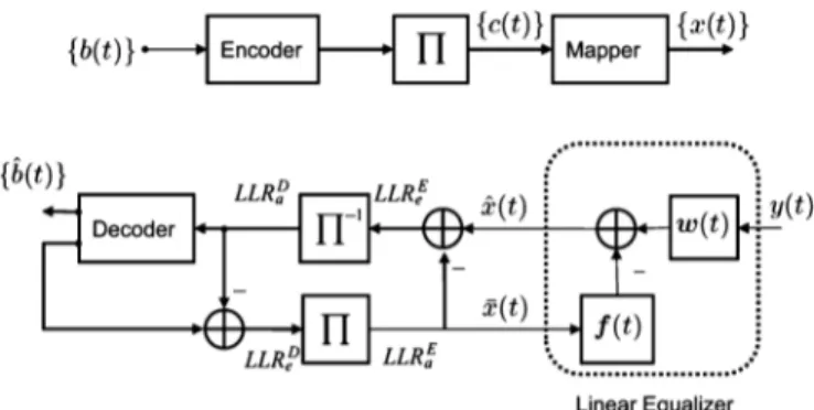
The block diagram of the system we consider with a linear turbo equalizer is shown in Fig. 2. The information bits are first encoded using an error correcting code (ECC) and then interleaved to generate . The interleaved code bits are transmitted after symbol

mapping, e.g., for BPSK signaling, through

a baseband discrete-time channel with a finite-length

im-pulse response , , represented by

. The communication channel is unknown. The transmitted signal is assumed to be uncorrelated due to the interleaver. The received signal is given by

where is the additive complex white Gaussian noise with zero mean and circular symmetric variance . If a linear equal-izer is used to reduce the ISI, then the estimate of the desired data, i.e., , using the received data is given by

where is length

linear equalizer, and

note that we use negative indices with a slight abuse of notation.

The received data vector is given by ,

where and

Fig. 2. Block diagram for a bit interleaved coded modulation transmitter and receiver with a linear turbo equalizer.

is the convolution matrix corresponding to , the estimate of can be written as

(1) given that the mean of the transmitted data is known.

However, in turbo equalization, instead of only using an equalizer, the equalization and the decoding are jointly per-formed iteratively at the receiver of Fig. 2. The equalizer computes the a posteriori information using the received signal, transmitted signal estimate, channel convolution matrix (if known) and a priori probability of the transmitted data. After subtracting the a priori information, , and de-inter-leaving the extrinsic information , a soft input soft output (SISO) channel decoder computes the extrinsic information on coded bits, which are fed back to the linear equalizer as a priori information after interleaving.

If one uses the linear MMSE equalizer in , the mean and the variance of are required to calculate and . These quantities are computed using the a priori

infor-mation from the decoder as 1

and . As an example,

for BPSK signaling, the mean and variance are given as

and . However, to

remove dependency of to due to using and

in (1), one can set while computing ,

yielding and [5]. Then, the linear MMSE

equalizer is given by

(2)

where is

a diagonal matrix (due to uncorrelateness assumption on )

with diagonal entries ,

, is

the th column of , is the reduced form of

where the th column is removed. The linear MMSE equalizer in (1) yields

(3)

1_{With a slight abuse of notation, the expression is interpreted}

here and in the sequel as the expectation of with respect to the prior distri-bution .

where . In this sense the linear MMSE equalizer can be decomposed into a feedforward filter processing

and a feedback filter processing .

Remark 1: Both the linear MMSE feedforward and feedback

filters are highly nonlinear functions of , i.e.,

(4)

where . We point out that time

variation in (2) is due to the time variation in the vector of vari-ances (assuming is time-invariant).

To learn the corresponding feedforward and feedback filters that are highly nonlinear functions of , we use piecewise linear models based on vector quantization and context trees in the next section. The space spanned by is partitioned into disjoint regions and a separate linear model is trained for each region to approximate functions and using piecewise linear models.

Note that if the channel is not known or estimated, one can directly train the corresponding equalizers in (3) using adaptive algorithms such as in [4], [12] without channel estimation or piecewise constant partitioning as done in this paper. In this case, one directly applies the adaptive algorithms to feedforward and feedback filters using the received data and the mean vector as feedback without considering the soft decisions as a priori probabilities. Assuming stationarity of , such an adaptive feedforward and feedback filters have Wiener solutions [12]

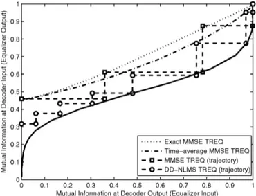
(5) Note that assuming stationarity of the log likelihood ra-tios [12], is constant in time, i.e., no time index for , in (5). When PSK signaling is used such that , the filter coefficient vector in (5) is equal to the coefficient vector of the MMSE equalizer in [5] with the time averaged soft information, i.e., time average instead of an ensemble mean. Comparing (5) and (2), we observe that using the time averaged soft information does not degrade equalizer performance in the no a priori information, i.e., or perfect a priori information, i.e., , cases. In addition, the performance degradation in moderate ISI channels is often small [5] when perfect channel knowledge is used. However, the performance gap increases in ISI channels that are more difficult to equalize, even in the high SNR region [12], since the effect of the filter time variation increases in the high SNR region. Comparison of an exact MMSE turbo equalizer without channel estimation error and an MMSE turbo equalizer with the time averaged soft variances (i.e. when an ideal filter for the converged adaptive turbo equalizer is used) via the EXIT chart [22] is given in Fig. 3. As the adaptive turbo equalizer, a decision directed (DD) LMS turbo equalizer is used in the data transmission period, while LMS is run on the received signals for the first turbo iteration and on the received signals and training symbols for the rest of turbo iterations in the training period. Note that the tentative decisions can be

Fig. 3. The EXIT chart for the exact MMSE turbo equalizer, the LMS turbo equalizer and their trajectory in a time invariant ISI channel . Here, we have , ,

, feedback filter length , ,

, , BPSK signaling, random inter-leaver and rate convolutional code with constraint length of 3.

taken as the hard decisions at the output of the linear equalizer or as the soft decisions from the total LLRs at the output of decoder. When we consider nonideality, both of the MMSE turbo equalizer with channel estimation error and DD-LMS turbo equalizer loose mutual information at the equalizer in first few turbo iterations.2_{Even though there is a loss in mutual}

information at the equalizer in the first and second turbo itera-tion due to using decision directed data or channel estimaitera-tion error, both algorithms follow their ideal performance at the end. (i.e., the DD LMS turbo equalizer can achieve the performance of the time-average MMSE turbo equalizer as the decision data gets more reliable). However, there is still a gap in achieved mutual information between the exact MMSE turbo equalizer and the LMS adaptive turbo equalizer except for the no a

priori information and perfect a priori information cases. Note

that such a gap can make an adaptive turbo equalizer become trapped at lower SNR region while an MMSE turbo equalizer converges as turbo iteration increases.

To remedy this, in the next section, we introduce piecewise linear equalizers to approximate and . We first dis-cuss adaptive piecewise linear equalizers with a fixed partition

of (where ). Then, we introduce

adap-tive piecewise linear equalizers using context trees that can learn the best partition from a large class of possible partitions of

.

III. NONLINEARTURBOEQUALIZATIONUSING

PIECEWISELINEARMODELS

A. Piecewise Linear Turbo Equalization with Fixed Partitioning

In this section, we divide the space spanned by (assuming BPSK signaling for notational sim-plicity) into disjoint regions , e.g.,

2_{This performance loss in the first few turbo iterations can cause the iterative}

for some and train an independent linear equalizer in each region to yield a final piecewise linear equalizer to

approxi-mate and . As an example, given such

regions, suppose a time varying linear equalizer is assigned to

each region as , , , such that at each

time , if , the estimate of the received signal is given as

(6) We emphasize that the time variations in and in (6) are not due to the time variation in unlike (3). The fil-ters and are time varying since they are produced by adaptive algorithms sequentially learning the corresponding functions and in region . Note that if is large and the regions are dense such that (and ) can be consid-ered constant in , say equal to for some in region , then if the adaptation method used in each region converges

successfully, this yields and

as . Hence, if these regions are dense and there is enough data to learn the corresponding models in each region, then this piecewise model can approximate any smoothly varying

and [23].

In order to choose the corresponding regions , we apply a vector quantization (VQ) algorithm to the sequence of , such as the LBG VQ algorithm [24]. If a VQ algorithm with regions and Euclidean distance is used for clustering, then the centroids and the corresponding regions are defined as (7) (8) where

, and . We emphasize that we

use a VQ algorithm on to construct the corresponding partitioned regions in order to concentrate on vectors that are

in since and should only be learned around

, not for all . After the regions are con-structed using the VQ algorithm and the corresponding filters in each region are trained with an appropriate adaptive method,

the estimate of at each time is given as if

.

In Fig. 4, we introduce such a sequential piecewise linear equalizer that uses the LMS update to train its equalizer filters. Here, is the learning rate of the LMS updates. One can use dif-ferent adaptive methods instead of the LMS update, such as the RLS or NLMS updates [25], by only changing the filter update steps in Fig. 4. The algorithm of Fig. 4 has access to training data of size . After the training data is used, the adaptive methods work in decision directed mode [25]. Since there are no a priori probabilities in the first turbo iteration, this algorithm uses an LMS update to train a linear equalizer with only the feedforward filter, i.e., , without any regions or mean vec-tors. Note that an adaptive feedforward linear filter trained on only without a priori probabilities (as in the first itera-tion) converges to [12] (assuming zero variance in convergence)

which is the linear MMSE feedforward filter in (2) with .

In the pseudo-code in Fig. 4, the iteration numbers are dis-played as superscripts, e.g., , are the feedfor-ward and feedback filters for the th iteration corresponding to the th region, respectively. After the first iteration when become available, we apply the VQ algorithm to get the corresponding regions and the centroids. Then, for each re-gion, we run a separate LMS update to train a linear equal-izer and construct the estimated data as in (6). In the start of the second iteration, in line A, each feedforward filter is initial-ized by the feedforward filter trained in the first iteration. Fur-thermore, although the linear equalizers should have the form , since we have the correct in the training mode for , the algorithms are trained using

in (line B), i.e., is scaled using , to incorporate the uncertainty during training [26]. After the second iteration, in the start of each iteration, in line C, the linear equalizers in each region, say , are initialized using the filters trained in the previous iteration that are closest to the th region, i.e.,

, , and .

Assuming large with dense regions, we have

when . To get the vectors that the LMS trained linear filters in region eventually converge, i.e., the linear MMSE es-timators assuming stationary , we need to calculate

, which is assumed to be diag-onal due to the interleaving [12], yielding

due to the definition of and assuming stationary distribution on . This yields that the linear filters in region converge to

(9) where , assuming zero variance at convergence. Hence, at each time , assuming convergence, the difference between the MSE of the equalizer in (9) and the MSE of the linear MMSE equalizer in (2) is given by

(10) as shown in Appendix A. Due to (10) as the number of piecewise linear regions, i.e., , increases and approaches 0, the MSE of the converged adaptive filter more accurately approximates the MSE of the linear MMSE equalizer.

Note that the algorithm in Fig. 4 uses the LBG VQ for clus-tering and separate piecewise linear equalizers, one for each

Fig. 4. A piecewise linear equalizer for turbo equalization. This algorithm requires computations.

region. At the start of each turbo iteration, the LBG VQ

algo-rithm requires computations [24], where

is the number of clusters, is the data length, is the size of each variance vector and is an upper bound on the number of iterations that the LBG VQ requires for conver-gence. Then, at each time , the LBG VQ requires

computations, i.e., number of

addi-tions and multiplicaaddi-tions.3_{At each time , after observing ,}

the algorithm requires computations to find

the region that belongs to, computations to

calculate the output for that region and compu-tations to update the piecewise linear equalizer for that regions with the LMS algorithm. Hence, for each time (or per each output), the algorithm in Fig. 4 requires

computations.

In the algorithm of Fig. 4, the partition of the space of is fixed, i.e., partitioned regions are fixed at the start of the equalization, after the VQ algorithm, and we

sequen-3_{If the complexity of the LBG is significant compared to the adaptive}

algo-rithms, then one can replace it with a more appropriate partitioning method. As an example, the complexity of the LBG VQ can be significantly reduced by changing the distance measure to the Chaudhuris distance [27] instead of the Euclidian distance, which requires no multiplications.

tially learn a different linear equalizer for each region. Since the equalizers are sequentially learned with a limited amount of data, these may cause training problems if there is not enough data in each region. In other words, although one can increase to increase approximation power, if there is not enough data to learn the corresponding linear models in each region, this may deteriorate the performance. To alleviate this, one can try a piecewise linear model with smaller in the start of the learning and gradually increase to moderate values if enough data is available. In the next section, we examine the context tree weighting method that intrinsically does such weighting among different models based on their performance, hence, allowing the boundaries of the partition regions to be design parameters.

B. Piecewise Linear Turbo Equalization Using Context Trees

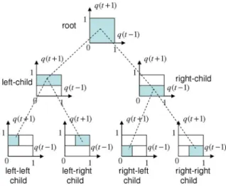
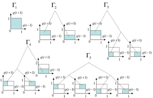
We first introduce a binary context tree to partition the side information space, , into disjoint regions. An ex-ample binary context tree is provided in Fig. 5. In a binary con-text tree, starting from the root node, i.e., the top node, we have a left hand child and a right hand child. Each left hand child and right hand child have their own left hand and right hand chil-dren. This splitting yields a binary tree of depth with a total

Fig. 5. A full binary context tree with depth, , with 4 leaves. The leaves of this binary tree partitions , i.e., , into 4 disjoint regions.

of leaves at depth and a total of nodes including the root and the leaves. The example context tree in Fig. 5 has

and partitions , i.e.,

, into 4 disjoint regions. Each one of these 4 disjoint re-gions is assigned to a leaf in this binary tree. Then, recursively, each internal node on this tree represents a region (shaded areas in Fig. 5), which is the union of the regions assigned to its chil-dren. Each node of the context tree represents a certain region (or part) of the side information space.

Using a binary context tree of depth , one can represent a doubly exponential number, , of different “parti-tions” of the side information space. As an example, in Fig. 6, we provide the five partitions that can be represented by our bi-nary tree with labeled as . Each partition rep-resented by this context tree is assigned to a “complete” subtree. A complete subtree is constructed from a subset of the nodes of the original tree, starting from the same root node, and the union of the regions assigned to the leaves of the subtree yields . For example, the subtree, in Fig. 6, which has the left-child, the right-left child and the right-right child as its leaves provides a complete partition of . For any subtree defined in the binary tree, if the regions assigned to its

leaves are labeled as where is the number of

leaves of the subtree , then . Each

of the subtree corresponds to a node in the original tree. To construct our context tree based piecewise linear equal-izer, we first partition the side information space with the LBG VQ algorithm as in the previous section and then construct our context tree over these regions as follows. We emphasize that the context tree is not directly used to partition the side infor-mation space but rather represents the possible partitions that can be constructed as the union of the final regions produced by the LBG VQ. Suppose the LBG VQ algorithm is applied to with to generate regions [24]. These regions are assigned to the leaves of a binary context tree of depth . Then, recursively, each internal node represents a region, which is the union of its children nodes. Note that one can arbitrarily assign the regions produced by the LBG VQ to the leaves of the context tree. However, the LBG VQ algorithm uses a tree notion

similar to the context tree introduced in Fig. 6 such that the LBG VQ algorithm intrinsically constructs the context tree. The LBG VQ algorithm starts from a root node and calculates the mean of all the vectors in as the root codeword, and binary splits the data as well as the root codeword into two segments. Then, these newly constructed codewords are iteratively used as the initial codebook of the split segments. These two code-words are then split in four and the process is repeated until the desired number of regions are reached. At the end, this binary splitting and clustering yield regions with the corresponding centroids , , which are assigned to the leaves of the context tree. Note that since each couple of the leaves (or nodes) come from a parent node after a binary splitting, these parent codewords are stored as the internal nodes of the context tree, i.e., the nodes that are generated by splitting a parent node are considered as siblings of this parent node where the centroid before splitting is stored. Hence, in this sense, the LBG VQ al-gorithm constructed the context tree.

Given such a context tree, we have different partitions of the space and can construct a piece-wise linear equalizer, say , as in Fig. 4 for each such parti-tion. One of these partitions, with the piecewise adaptive linear model defined on it achieves the minimal loss, e.g., the

min-imal accumulated squared error ,

for some . However, the best piecewise model with the best partition is not known a priori. We point out that although we have a doubly exponential number of piecewise linear models defined on the context tree, all these piecewise linear equalizers are constructed using subsets of nodes

of the tree. Hence, suppose we number each node on this

con-text tree and assign a linear equalizer

to each node as . The linear

models , that are assigned to node , train only on the data assigned to that node as in Fig. 4, i.e., if is in the re-gion that is assigned to the node , say , then and are updated. Then, the piecewise linear equalizer

corre-sponding to any partition is defined such

that if and is the node that is assigned to , i.e., , then

(11) We emphasize that this observation is critical while we intro-duce an algorithm that achieves the performance of the best par-tition with the best linear model that achieves the minimal ac-cumulated square-error with complexity only linear in the depth of the context tree per sample, i.e., complexity

instead of , where is the depth of the

tree.

Remark 2: We note that the partitioned model that

corre-sponds to the union of the leaves, i.e., the finest partition, has the finest partition of the space of variances. Hence, it has the highest number of regions and parameters to model the non-linear dependency. However, note that at each such region, the finest partition needs to train the corresponding linear equalizer that belongs to that region. As an example, the piecewise linear equalizer with the finest partition may not yield satisfactory re-sults in the beginning of the adaptation if there is not enough data to train all the model parameters. In this sense, as will be

Fig. 6. All partitions of using binary context tree with . Given any partition, the union of the regions represented by the leaves of each partition is equal to .

shown, the context tree algorithm adaptively weights coarser and finer models based on their performance.

To accomplish this, we introduce the algorithm in Fig. 7, i.e., , that is constructed using the context tree weighting method introduced in [15]. The context tree based equalization algorithm implicitly constructs all , , piece-wise linear equalizers and acts as if it had actually run all these equalizers in parallel on the received data. At each time , the final estimation is constructed as a weighted combina-tion of all the outputs of these piecewise linear equalizers as

(12) where the combination weights are calculated proportional to the performance of each equalizer on the past data

as explained in detail in Appendix B. However, as shown in (11) and explained in Appendix B, although there are different piecewise linear algorithms, at each time , each is equal to one of the node estimations to which belongs. Hence, (12) can be implemented as a combination of only outputs as

with certain combination weights and nodes . How the context tree algorithm keeps the track of these piecewise linear models as well as their performance-based combination weights with computational complexity only linear in the depth of the context tree is explained in Appendix B.

For the context tree algorithm, since there are no a priori probabilities in the first iteration, the first iteration of Fig. 7 is the same as the first iteration of Fig. 4. After the first iteration, to in-corporate the uncertainty during training as in Fig. 4, the context

tree algorithm is run by using weighted training data [26]. At each time , constructs its nonlinear estimation of as follows. We first find the regions to which belongs. Due to the tree structure, one needs only find the leaf node in which lies and collect all the parent nodes towards the root node. The nodes to which belongs are stored in in Fig. 7. The final estimate is constructed as a weighted com-bination of the estimates generated in these nodes, i.e., , , where the weights are functions of the performance of the node estimates in previous samples.

For the algorithm in Fig. 7, at the start of each turbo itera-tion, we need to perform LBG VQ clustering, which requires computations, i.e., additions and multiplications, for each time . For each time , we first need to find the nodes where belongs to, which requires

computations (since due to the tree structure finding the leaf where belongs to is enough). Then, we need to perform computations to calculate and combine the out-puts of each node equalizer and require compu-tations to update the piecewise linear equalizers at these nodes. Hence, for each time (or per each output), the algorithm in Fig. 7 requires

computations.

Theorem 2: Let , and represent the transmitted, noise and received signals and represents the sequence of variances constructed using the a priori prob-abilities for each constellation point produced by the SISO

decoder. Let , , are estimates of

produced by the equalizers assigned to each node on the context tree. The algorithm , when applied to , for all achieves

(13)

for all , , assuming perfect feedback

in decision directed mode i.e., when ,

is the node assigned to the volume in

such that belongs and is the number of regions in . If the estimation algorithms assigned to each node are selected as adaptive linear equalizers such as an RLS update based algo-rithm, (13) yields

(14) where is an indicator variable for such that if

, then .}

An outline of the proof of this theorem is given in Appendix B.

Remark 3: We observe from (13) that the context tree

al-gorithm achieves the performance of the best sequential rithm among a doubly exponential number of possible algo-rithms corresponding to all partitions. Note that the bound in (13) holds uniformly for all , however the bound is the largest for the finest partition, i.e., for the piecewise linear equalizer constructed using the regions assigned to the leaves. We ob-serve from (14) that the context tree algorithm also achieves the performance of even the best piecewise linear model, in-dependently optimized in each region, for all when the node estimators in each regions are adaptive algorithms that achieve the minimum least square-error.

C. MSE Performance of the Context Tree Equalizer

To get the MSE performance of the context tree equalizer, we observe that the result (14) in the theorem is uniformly true for any sequence . Hence, as a corollary to the theorem, taking the expectation of both sides of (14) with respect to any distribution on yields the following:

Corollary:

(15) Equation (14) is true for all , and given for any , ,

, i.e.,

(16)

since (14) is true for the minimizing and equalizer vectors. Taking the expectation of both sides of (16) and minimizing

with respect to and , , yields the

corol-lary.

We emphasize that the minimizer vectors and at the right hand side of (15) minimize the sum of all the MSEs. Hence, the corollary does not relate the MSE performance of the CTW equalizer to the MSE performance of the linear MMSE equalizer given in (2). However, if we assume that the adaptive filters trained at each node converge to their optimal coefficient vectors with zero variance and for sufficiently large and , we have piecewise linear models such as for the finest partition

(17) where we assumed that, for notational simplicity, the th

par-tition is the finest parpar-tition, and are

the MSE optimal filters (if defined) corresponding to the regions assigned to the leaves of the context tree. Note that we require to be large such that we can assume to be constant in each region such that these MSE optimal filters are well-de-fined. Since (14) is correct for all partitions and for the mini-mizing , vectors, (14) holds for any and ’s pairs including and pair. Since (14) in the theorem is uniformly true, taking the expectation preserves the bound and using (17), we have

(18) since for the finest partition . Using the MSE defini-tion for each node in (18) yields

(19)

(20) where (20) follows from assuming large , the MSE in each node is bounded as in (10), i.e.,

. Note that at the right hand

Fig. 7. A context tree based turbo equalization. This algorithm requires computations.

large enough with the partition given in Fig. 5 since we have

regions and . Hence, as ,

the context tree algorithm asymptotically achieves the perfor-mance of the linear MMSE equalizer, i.e., the equalizer that is nonlinear in the variances of the soft information. However, for this to happen, the sample length should go faster to infinity than as seen from the last term in (20).

IV. NUMERICALEXAMPLES

In the following, we simulate the performance of our algo-rithms under different scenarios. A rate one half convolutional code4_{with constraint length 3 and random interleaving is used.}

4_{A recursive systematic convolutional code with a generator matrix [101;111]}

is used and Log-MAP decoding algorithm is considered as a decoding algorithm in this paper.

Fig. 8. Ensemble averaged MSE for the CTW equalizer over 5 turbo iterations at 12 dB Eb/N0.

In the first set of experiments, we use the time invariant chan-nels from [8] (Chapter 10)

with the training size and data length 5120 (ex-cluding training). Training symbols are modulated with same modulation order of data symbols without encoding. We use two different adaptive algorithms including the LMS algorithm and the normalized LMS algorithm (NLMS) [28]. The decision directed mode is used for all the adaptive algorithms, e.g., for the ordinary LMS turbo equalizer we compete against and for all the node filters on the context tree. Our calculation of the extrinsic LLR at the output of the ordinary LMS algorithm is based on [10]. For all adaptive filters, we use , ,

length feedback filter. The learning rates

for the LMS and the NLMS algorithms are set to

and , respectively. These learning rates are selected to guarantee the convergence of the ordinary LMS and NLMS filter in the training part. The same learning rate is used directly on the context tree without tuning for fair comparison.

As shown in Fig. 8, the MSE of the CTW equalizer decreases as the depth of the CTW increases as shown in (10). We also increase the data length as , since the MSE of the CTW equalizer depends on both the depth of the context tree and the data length as demonstrated in (20). Furthermore, the MSEs of the linear MMSE TREQ and the linear MMSE TREQ with the finest partitioning are plotted as references, where the ideal channel estimation is assumed. Note that the difference be-tween the MSE of the linear TREQ constructed using the finest partitioning and the MSE of the linear MMSE TREQ is bounded by the quantization error as shown in (10), where convergence of the linear filters for the finest partitioning is assumed. For the converged linear TREQ with the finest partitioning, we use the linear MMSE TREQ with the finest partition as the genie aided method. Note that, as expected, the MSE of the linear MMSE TREQ with the finest partition also decreases as the CTW depth increases since the quantization error decreases as the depth creases, i.e., the number of regions in the finest partition in-creases, where quantization level is given by .

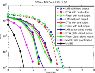
Fig. 9. BERs for an ordinary DD LMS algorithm, a CTW equalizer with and tree given in Fig. 5, the piecewise equalizer with the finest partition, i.e.,

. (BPSK at the th turbo iteration in the ISI channel, ).

In Fig. 9, we plot BERs for an ordinary LMS algorithm, a con-text-tree equalization algorithm with given in Fig. 7 and the piecewise linear equalization algorithm with the finest parti-tion, i.e., , on the same tree. In a decision directed mode, hard decision data, soft decision data are used in these simula-tions. Data-aided adaptive algorithms are also demonstrated to show the ideal performance of the adaptive algorithms. As a reference, BERs of the MMSE TREQ and the MMSE TREQ with finest partition, where we assume that channel information is perfectly known at the receiver side. Note that the piecewise linear equalizer with the finest partition, i.e., , in Fig. 6, has the finest partition with the highest number of linear models, i.e., independent filters, for equalization. However, we em-phasize that all the linear filters in the leaves should be se-quentially trained for the finest partition. Hence, as explained in Section III-B, the piecewise linear model with the finest par-tition may yield inferior performance compared to the CTW al-gorithm that adaptively weights all the models based on their performance. We observe that the context tree equalizer out-performs the ordinary LMS equalizer and the equalizer corre-sponding to the finest partition in the hard output result.

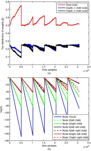
In Fig. 10, we plot the weight evaluation of the context tree algorithm, i.e., the combined weight in line F of Fig. 7, to show the convergence of the CTW algorithm. Note that the combined weight vector for the CTW algorithm is only defined over the data length period 5120 at each turbo iteration, i.e., the com-bined weight vector is not defined in the training period. We collect the combined weight vectors for the CTW algorithm in the data period for all iterations and plot them in Fig. 10. This results in jumps in the figure, since at each discontinuity, i.e., after the data period, we switch to the training period and con-tinue to train the node filters. The context tree algorithm, un-like the finest partition model, adaptively weights different par-titions in each level. To see this, in Fig. 11(a), we plot weights assigned to each level in a depth context tree. We also plot the time evaluation of the performance measures in Fig. 11(b). We observe that the context tree algorithm, as ex-pected, at the start of the equalization divides the weights fairly uniformly among the partitions or node equalizers. However, naturally, as the training size increases, when there is enough

Fig. 10. Ensemble averaged combined weight vector for the CTW equalizer over turbo iterations.

Fig. 11. (a) The distribution of the weights, i.e., values assigned to , , such that belongs to th level. (b) Time evaluation of which represents the performance of the linear equalizer assigned to node . Note that at each iteration, we reset since a new tree is constructed using clustering.

Fig. 12. BER comparison in the case of 16QAM at the th turbo iteration in the ISI channel, .

Fig. 13. BER comparison in the case of 16QAM at the 7th turbo iteration in a randomly generated channel with length 15.

data to train all the node filters, the context tree algorithm fa-vors models with better performance. Note that at each iteration, we reset node probabilities since a new tree is con-structed using clustering.

As the next set of experiments, we perform BER performance comparison under 16QAM modulation with the time invariant ISI channel, . The BER results are plotted in Fig. 12, where the NLMS TREQ is used with . We observe that BERs of adaptive algorithms with soft decision data or data-aided adaptive algorithms are close to the ideal MMSE equalizer. In the data-aided mode, the CTW algorithm is better than the other adaptive algorithms. To show the performance in a long delay spread channel, we performed experiments on a randomly gen-erated channel of length 15 and provide the BER performance in Fig. 13. We observe similar performance improvement with the CTW algorithm in BER for this randomly generated channel as expected from our derivations.

V. CONCLUSION

In this paper, we introduced an adaptive nonlinear turbo equalization algorithm using context trees to model the non-linear dependency of the non-linear MMSE equalizer on the soft information generated from the decoder. We use the CTW algorithm to partition the space of variances, which are time dependent and generated from the soft information. We demon-strate that the algorithm introduced asymptotically achieves the performance of the best piecewise linear model defined on this context tree with a computational complexity only of the order of an ordinary linear equalizer. We also demonstrate the convergence of the MSE of the CTW algorithm to the MSE of the linear minimum MSE estimator as the depth of the context tree and the data length increase.

APPENDIXA

To calculate the difference between the MSE of the equalizer in (9) and the MSE of the linear MMSE equalizer in (2), we start with

(21)

where (and the time index in is omitted

for presentation purposes) and .

To simplify the second term in (21), we use the first order ex-pansion from the Lemma in the last part of Appendix A to yield

(22)

(23) around . Hence using (23) in (21) yields

(24) where the last line follows from the Schwartz inequality.

Lemma: We have [21]

(25)

Proof: To get the gradient of

with respect to , we differentiate the identity with respect to , i.e., the th and th element of the matrix and obtain

where is a vector of all zeros except a single 1 at th entry. This yields

(26) which yields the result in (25) since (26) is the th element of the matrix in (25).

APPENDIXB

Outline of the proof of the theorem 2: The proof of the

the-orem follows the proof of the Thethe-orem 2 of [19] and Thethe-orem 1 of [29]. Hence, we mainly focus on differences.

Suppose we hypothetically construct all piecewise linear

equalizers , defined on the context tree and

compute certain weights for all

(27)

where are constants that are used only

for proof purposes such that [15] and is

a positive constant set to [29]. Note

that the weights defined in (27) are normalized functions of the performance of each on the observed data so far, i.e., the better performing piecewise linear equalizers would have higher weights. At each time , if we define a weighted equalizer

(28) then it follows from Theorem 1 of [29] that the performance of the weighted equalizer satisfies

for all . In this sense, is the desired , i.e., it achieves the performance of the best piecewise equal-izer among piecewise linear equalizers defined on the con-text tree. The proof that (28) satisfies (29) is based on defining universal probabilities, using telescoping and certain convexity arguments, however, straightforward and is not repeated here. However, even if we have the result in (29), note that re-quires the outputs of doubly exponential number algorithms and computes performance based weights in (27), which is computationally infeasible for large . We next show that such a doubly exponential number of algorithms and weights can be efficiently calculated on the context tree, i.e., the weighted sum-mation in (29) can be efficiently calculated because of the tree structure.

To circumvent this problem, we first observe that any defined in the binary tree is constructed from a subset of

node equalizers , . At each time

, for each partition , we find the corresponding node that belongs to and repeat the output of the corresponding to that node as the output of . However, at each time , due to the tree structure of the partitions, can only belong to regions or nodes on the tree. As an example, if belongs to the left-left hand child, then it also belongs to the left-hand child and the root node. For such a , all piecewise linear equalizers would equal to one of these three node outputs. In this sense, although we have piecewise equalizers in (27), these equalizers can only output distinct values, i.e., the outputs of the nodes that belongs. Hence, at each time , is constructed as a weighted sum of only distinct node predictions. Then, all the weights in (27) with the same node predictions can be merged.

To be able to define such a merging with computational com-plexity only linear in , as shown in [19], we define certain functions of performance for each node as , that are initialized in (line A) and updated in (line C), (line D), (line E) of Fig. 7. These variables measure the performance as in (27), where

is the performance of each node piecewise linear equalizer on the data observed so far, is the nodes assigned to the and

is the accumulated weight recursively calculated for each at the inner nodes, where and are the weights for each child node. Then, the corresponding can be defined as a merged summation of node outputs as

where contains the nodes that belongs to and are calculated as shown in (line B) of Fig. 7 based on and

. Hence, the desired equalizer is given by

which requires computing node estimations and updates only node equalizers at each time and store

node weights. This completes the outline of the proof of (13). To get the corresponding result in (14), we define the node predictors as the LS predictors such that

(30)

and , where

, is the indicator variable for node , i.e.,

if otherwise . The affine

pre-dictor in (30) is a least squares prepre-dictor that trains only on the observed data and that belongs to that node, i.e., that falls into the region . Note that the update in (30) can be implemented with computations using fast inversion methods [30]. For each node , the RLS algorithm is shown to achieve the excess loss

(31) where is the number of samples that fall into the node . Hence, application of this results to each node predictor in (29) yields the result in (14) as shown in [31].

REFERENCES

[1] C. Douillard, M. Jezequel, C. Berrou, A. Picart, P. Didier, and A. Glavieux, “Iterative correction of inter-symbol interference: Turbo equalization,” Eur. Trans. Telecommun., vol. 6, no. 5, pp. 507–511, Sep.–Oct. 1995.

[2] J. Hagenauer, “The turbo principle: Tutorial introduction and state of the art,” in Proc. Int. Symp. Turbo Codes, Brest, France, 1997, pp. 1–11. [3] C. Berrou and A. Glavieux, “Near optimum error correcting coding and decoding: Turbo codes,” IEEE Trans. Commun., vol. 44, pp. 1261–1271, Oct. 1996.

[4] A. Glavieux, C. Laot, and J. Labat, “Turbo equalization over a fre-quency selective channel,” in Proc. Int. Symp. Turbo Codes, Brest, France, 1997, pp. 96–102.

[5] M. Tüchler, R. Koetter, and A. C. Singer, “Turbo equalization: Prin-ciples and new results,” IEEE Trans. Commun., vol. 50, no. 5, pp. 754–767, May 2002.

[6] S. Song, A. C. Singer, and K.-M. Sung, “Soft input channel estimation for turbo equalization,” IEEE Trans. Signal Process., vol. 52, no. 10, pp. 2885–2894, Oct. 2004.

[7] C. Studer, S. Fateh, and D. Seethaler, “Asic implementation of soft-input soft-output MIMO detection using parallel interference cancella-tion,” IEEE J. Solid-State Circuits, vol. 56, no. 7, pp. 1754–1765, Jul. 2011.

[8] J. Proakis, Digital Communications. New York, NY, USA: McGraw-Hill, 1995.

[9] C. Laot, R. Le Bidan, and D. Leroux, “Low-complexity MMSE turbo equalization: A possible solution for EDGE,” IEEE Trans. Wireless

Commun., vol. 4, no. 3, pp. 965–974, May 2005.

[10] J. W. Choi, R. J. Drost, A. C. Singer, and J. Preisig, “Iterative mul-tichannel equalization and decoding for high frequency underwater acoustic communications,” in Proc. IEEE Sensor Array Multichannel

Signal Process. Workshop, 2008, pp. 127–130.

[11] A. C. Singer, J. K. Nelson, and S. S. Kozat, “Signal processing for underwater acoustic communications,” IEEE Commun. Mag., vol. 47, no. 1, pp. 90–96, Jan. 2009.

[12] R. Le Bidan, “Turbo-equalization for bandwith-efficient digital com-munications over frequency-selective channels,” Ph.D. dissertation, In-stitut TELECOM/TELECOM, Bretagne, France, 2003.

[13] M. Tüchler, “Iterative Equalization Using Priors,” M.Sc. thesis, Univ. of Illinois at Urbana-Champaign, Urbana, IL, USA, 2000.

[14] M. Tüchler, A. C. Singer, and R. Koetter, “Minimum mean squared error equalization using priors,” IEEE Trans. Signal Process., vol. 50, no. 3, pp. 673–683, Mar. 2002.

[15] F. M. J. Willems, “Coding for a binary independent piecewise-iden-tically-distributed source,” IEEE Trans. Inf. Theory, vol. 42, pp. 2210–2217, Nov. 1996.

[16] S. S. Kozat and A. C. Singer, “Universal switching linear least squares prediction,” IEEE Trans. Signal Process., vol. 56, pp. 189–204, Jan. 2008.

[17] D. P. Helmbold and R. E. Schapire, “Predicting nearly as well as the best pruning of a decision tree,” Mach. Learn., vol. 27, no. 1, pp. 51–68, Apr. 1997.

[18] E. Takimoto, A. Maruoka, and V. Vovk, “Predicting nearly as well as the best pruning of a decision tree through dyanamic programming scheme,” Theoretic. Comput. Sci., vol. 261, pp. 179–209, June 2001. [19] S. S. Kozat, A. C. Singer, and G. C. Zeitler, “Universal piecewise linear

prediction via context trees,” IEEE Trans. Signal Process., vol. 55, pp. 3730–3745, Jul. 2007.

[20] Y. Yilmaz and S. S. Kozat, “Competitive randomized nonlinear pre-diction under additive noise,” IEEE Signal Process. Lett., vol. 17, no. 4, pp. 335–339, Apr. 2010.

[21] A. Graham, Kronecker Products and Matrix Calculus: With

Applica-tions. Chichester, U.K.: Ellis Horwood, 1981.

[22] S. Lee, A. C. Singer, and N. R. Shanbhag, “Linear turbo equaliza-tion analysis via BER transfer and EXIT charts,” IEEE Trans. Signal

Process., vol. 53, pp. 2883–2897, Aug. 2005.

[23] O. J. J. Michel, A. O. Hero, and A. E. Badel, “Tree structured non-linear signal modeling and prediction,” IEEE Trans. Signal Process., pp. 3027–3041, Nov. 1999.

[24] A. Gersho and R. M. Gray, Vector Quantization and Signal

Compres-sion, ser. Springer Int. Series in Engineering and Computer Science.

New York, NY, USA: Springer, 1992.

[25] S. Haykin, Adaptive Filter Theory. Englewood Cliffs, NJ, USA: Prentice-Hall, 1996.

[26] K. Kim, J. W. Choi, A. C. Singer, and K. Kim, “A new adaptive turbo equalizer with soft information classification,” in Proc. Int.

Conf. Acoust., Speech, Signal Process., Dallas, TX, USA, 2010, pp.

3206–3209.

[27] D. P. Chaudhuri, C. A. Murthy, and B. B. Chaudhuri, “A modified metric to compute distance,” Pattern Recognit., vol. 25, no. 7, pp. 667–677, Jul. 1992.

[28] A. H. Sayed, Fundamentals of Adaptive Filtering. New York, NY, USA: Wiley, 2003.

[29] A. C. Singer and M. Feder, “Universal linear prediction by model order weighting,” IEEE Trans. Signal Process., vol. 47, no. 10, pp. 2685–2699, Oct. 1999.

[30] J. Cioffi and T. Kailath, “Fast recursive least squares traversal filters for adaptive filtering,” IEEE Trans. Acoust., Speech, Signal Process., vol. 32, pp. 304–337, Nov. 1984.

[31] N. Merhav and M. Feder, “Universal schemes for sequential decision from individual sequences,” IEEE Trans. Inf. Theory, vol. 39, no. 4, pp. 1280–1292, Jul. 1993.

Kyeongyeon Kim (M’07) received the B.S., M.S., and Ph.D. degrees in electrical engineering from Yonsei University, Seoul, Korea, in 2001, 2003 and 2007, respectively.

After graduation, she was a Postdoctoral Fellow in Purdue University, West Lafayette, IN, USA, from 2007 to 2008 and in the University of Illi-nois at Urbana-Champaign, USA, from 2008 to 2010. Since 2010, she has been with Samsung Advanced Institute of Technology (SAIT), Samsung Electronics, Yongin-si, Korea, and participated in low-power receiver algorithm design and software implementation of wireless communication and broadcasting systems. Her research interests include signal processing for wireless/underwater communication and broadcasting systems, array signal processing, and communication system anaysis and design.

Nargiz Kalantarova was born on October 29, 1985, in Baku, Azerbaijan. She received the B.S. degrees in both electrical engineering and mathematics from Bogazici University, Istanbul, Turkey, in 2008.

Currently, she is a Research Assistant and is working toward the M.S. degree at the Electrical and Computer Engineering in Koc University, Istanbul, Turkey. Her research interests include statistical signal processing, digital communications, and optimization.

Suleyman Serdar Kozat (SM’11) received the B.S. degree with full scholarship and high honors from Bilkent University, Ankara, Turkey, and the M.S. and Ph.D. degrees in electrical and computer engineering from the University of Illinois at Urbana Champaign, Urbana, IL, USA, in 2001 and 2004, respectively.

After graduation, he joined IBM Research, T. J. Watson Research Lab, Yorktown, NY, USA, as a Research Staff Member in the Pervasive Speech Technologies Group, where he focused on problems related to statistical signal processing and machine learning. While working on his Ph.D., he was also working as a Research Associate at Microsoft Research, Redmond, WA, USA, in the Cryptography and Anti-Piracy Group. He holds several patent inventions due to his research accomplishments at IBM Research and Microsoft Research. After serving as an Assistant Professor at Koc University, Istanbul, Turkey, he is currently an Assistant Professor (with the Associate Professor degree from Yuksek Ogretim Kurumu) at the Electrical And Electronics Department of Bilkent University. Overall, his research interests include signal processing, adaptive filtering, sequential learning, and machine learning.

Dr. Kozat has been serving as an Associate Editor for the IEEE TRANSACTIONS ON SIGNAL PROCESSING (and he is currently the only Associate Editor in Turkey for this top ranking signal processing journal). He is the General Co-Chair for the IEEE Machine for Signal Processing, Istanbul, Turkey, 2013. He has been awarded the IBM Faculty Award by IBM Research in 2011, the Outstanding Faculty Award by Koc University in 2011 (granted the first time in 16 years), the Outstanding Young Researcher Award by the Turkish National Academy of Sciences in 2010, the ODTU Prof. Dr. Mustafa N. Parlar Research Encouragement Award in 2011, and holds Career Award by the Scientific Research Council of Turkey, 2009. He has also served in many Technical Committees of different international and national conferences and workshops. During his high school years, he won several scholarships and medals in international and national science and math competitions.

Andrew C. Singer (F’10) received the S.B., S.M., and Ph.D. degrees, all in electrical engineering and computer science, from the Massachusetts Institute of Technology (MIT), Cambridge, MA, USA.

Since 1998, he has been on the faculty of the Department of Electrical and Computer Engineering at the University of Illinois at Urbana-Champaign, IL, USA, where he is currently a Professor in the Electrical and Computer Engineering Department and the Coordinated Science Laboratory. During academic year 1996, he was a Postdoctoral Research Affiliate in the Research Laboratory of Electronics at MIT. From 1996 to 1998, he was a Research Scientist at Sanders, A Lockheed Martin Company, Manchester, NH, USA, where he designed algorithms, architectures, and systems for a variety of DOD applications. His research interests include signal processing and communication systems.

Dr. Singer was a Hughes Aircraft Masters Fellow, and was the recipient of the Harold L. Hazen Memorial Award for excellence in teaching in 1991. In 2000, he received the National Science Foundation CAREER Award; in 2001, he received the Xerox Faculty Research Award; and in 2002, he was named a Willett Faculty Scholar. He has served as an Associate Editor for the IEEE TRANSACTIONS ONSIGNALPROCESSINGand is a member of the MIT Educa-tional Council and of Eta Kappa Nu and Tau Beta Pi.