Non-interior piecewise-linear pathways to l-infinity solutions of overdetermined linear systems

··

's

-«и ν·'5^·:.;..-: ..

^

%✓ -.,ν,ΜΤ

«,*-'

■»:

J

.■ ..

XON-INTERIOR PIECEWISE-LLXEAR PATHW AY'S

TO

SOLUTIONS OF OVERDETERMIXED

LINEAR SYSTEMS

A THESIS

SUBMITTED TO THE DEPARTMENT OF INDUSTRIAL

ENGINEERING

AND THE INSTITUTE OF ENGINEERING AND SCIENCE

OF BILKENT UNIVERSITY

IN PARTIAL FULFILLMENT OF THE REQlTRExMENTS

FOR THE DEGREE OF

MASTER OF SCIENCE

By

Samir Elhedhli

June, 1996

Jamie....

/ J

I certify that I have read this thesis and that in my opinion it is fully adeciuate.

in scope and in quality, as a thesis for the degree of .Master of Science.

Pınar

(,\d visor)

I certify that I have read this thesis and that in my opinion it is fully adequate,

in scope and in quality, as a thesis for th^e degree of Master of Science.

I certify that I have read this thesis and that in my opinion it is fully adequate,

in scope and in quality, as a thesis for the degree of Master of Science.

Assist. Prof. Tuğrul Dayar

.Approved for the Institute of Engineering and Sciences:

Prof. Mehmet Krttay

(9л

(i 4-6.4

ABSTRACT

X O N -IN T E R IO R P I E C E W IS E -L IX E A R P A T H W A Y S T O

(y,

S O L U T IO N S O F O V E R D E T E R M IX E D L I X E A R S Y S T E M S

Samir Elhedhli

M .S. in Industrial Engineering

Supervisor: Assist. Prof. M ustafa Ç . Pınar

June. 1996

In this thesis, a new characterization of

solutions to overdetermined sys­

tems of linear equations is described based on a simple quadratic penalty func­

tion, which is used to change the problem into an unconstrained one. Piecewise-

linear non-interior pathways to the set of optimal solutions are generated from

the minimization of the unconstrained function. It is shown that the entire

set of

solutions is obtained from the paths for sufficiently small values of

a scalar parameter. As a consequence, a new finite penalty algorithm is given

for fx, problems. The algorithm is implemented and exhaustively tested us­

ing random and function approximation problems. .A comparison with the

Barrodale-Phillips algorithm is also done. The results indicate that the new

algorithm shows promising performance on random (non-function approxima­

tion) problems.

Key words:

Optimization; Overdetermined Linear Systems, Quadratic

Penalty Functions, Characterization.

ÖZET

D O Ğ R U S A L ^oc P R O B L E M İ İÇ İN BİR P A R Ç A L I

D O Ğ R U S A L DIŞ N O K T A A L G O R İT M A S I

Saınir Elhedhli

Endüstri Mühendisliği Bölüm ü Yüksek Lisans

Tez Yöneticisi: Yrd. Doç. Mustafa Ç. Pınar

Haziran, 1996

Bu tez çalışmasında, doğrusal

problemi için yeni bir algoritma önerilmiştir.

Algoritma karesel bir ceza fonksiyonunun problemin doğrusal programlama

formülasyonuna uygulanması ile elde edilmiştir. Karesel ceza fonksiyonunun

çözüm kümesi parçalı doğrusal bir yol izleyerek esas problemin ( ) çözüm

kümesine ulaşır. Algoritmanın sonlu sayıda adımda optimal çözüme ulaştığı

gösterilmiştir. .Algoritma bilgisayarda programlanmış ve değişik problemler

üzerinde denenmiştir. .Ayrıca optimizasyon literatüründe en iyi bilinen Barrodale-

Phillips simplex algoritması ile karşılaştırılmıştır.

Anahtar sözcükler:

Problemi, Doğrusal Sistemler, Karesel Ceza Fonksiy­

onu, Çözüm Kümesi Karakterizasyonu.

ACKNOWLEDGEMENT

I am indebted to Assist. Prof. Mustafa Ç. Pınar for his invaluable guidance,

encouragement and the enthusiasm which he inspired on me during this study.

I am also indebted to Assoc. Prof. Mustafa Akgül and Assist. Prof. Tuğrul

Dayar for showing keen interest on the subject matter and accepting to read

and review this thesis.

I would like to thank my office mates Alev Kaya and Murat Bayiz for their

patience and moral support.

I would like also to thank Abdullah Daşçı for his help during the preparation

of this thesis.

Finally, I would like to thank Fatma Gzara for everything.

Contents

1 Introduction

2

2 Literature Review

3

2 . 1

Historical Background ...

3

2 .2

The Algorithm of Barrodale and Phillips (1 9 7 -5 )...

4

2.3

The Algorithm of Bartels, Conn and Charalambous (1978) . . .

5

2.4

The Algorithm of Ruzinsky and Olsen (1989)

6

2.0

The .Algorithm of Coleman and Li (1 9 9 2 )...

S

2.6

Zhang’s -\lgorithm (1993)

9

3

A Quadratic Penalty Function Approach

11

3.1

Introduction...

1 1

3.2

Pathways To

Solutions

13

3.2.1

The Minimizers of F

...

14

3.2.2

Characterization of

S o lu t io n s ...

17

3.3

Extended Binary V ectors... 24

CONTENrS

vm

3.3

. 1

Behavior of the Set of Minitnizcrs near t he Feasible Bound­

ary

_2.5

3.4

The Penalty .Algorithm...

28

3.4.1

Computing an Unconstrained M in im ize!·...

>9

3.4.2

Reducing t ...

3

q

3.5

Finite C onvergence...

3

[

4 Example

₃₄

5 Numerical Issues and Implementation

38

5 .1

The Penalty A lgorithm ...

3 3

5.1.1

D e s crip tio n ...

3 3

5.1.2

Computing a minimizer of F (jr,y ,t)

39

5.1.3

Line S e a r c h ...

4 1

5.1.4

Reducing t ...

42

5.2

Implementation and Linear A lg e b ra ...

44

6

Numerical Testing

46

6.1

The Test P ro b le m s ... 46

6.2

Behavior of the algorithm ...

4

§

6.3

Initialization...

5 3

CONTENTS

7 Conclusion

IX

List of Figures

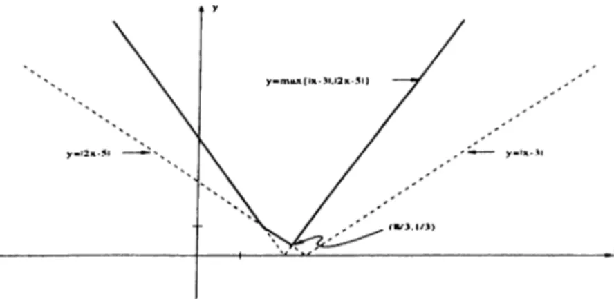
4.1

Plot of the function max(|r — 3|. |2jr — 5|)...

.34

4.2

The division of

according to the values of 0 i and

0 2

.

35

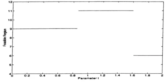
4.3

The region that contains the minimizer for different values of

t.

36

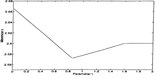
4.4

The minimizer x as a function of t ...

37

4.5

The minimizer

y as, s.

function of t ...

37

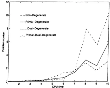
6.1

CPU time on nondegenerate, primal, dual and primal-dual de­

generate problems...

51

6.2

Comparison of the different initialization schemes of to...

63

6.3

CPU time comparison between LINFSOL and B-P for nonde­

generate problems... 63

6.4

CPU time comparison between LINFSOL and B-P for different

ratios of m to n on nondegenerate problems.

64

6.5

CPU time comparison for primal degenerate problems...64

6.6

CPU time ratio versus m to n ratio for primal degenerate prob­

lems... 65

6.7

CPU time comparison for dual degenerate problems.

65

LIST OF FIGURES

_XI

6.8

CPU time ratio versus m to

n

ratio for dual degenerate problems.

66

6.9 CPU time comparison for primal-dual degenerate problems.

66

6 .1 0

CPI time ratio versus

m

to

n

ratio for primal-dual degenerate

problems...

g j

Xl l

Glossary of Symbols and Notations

X

y

(■■»·, i/)

cL

a,

T

e

^ n + l

0

F{ z , t )

b

/1

0

Q

p

P

vector of length n.

scalar (€ -R).

pair of vector

x

and scalar

y.

(n

+ l)-vector with

Z{

=

X{

for i =

1

, ..,n and

=

y.

(n

+ l)-vector with d,; =

for

i =

and

=

dy.

j-th column of matrix

A.

¿-th row of matrix

A.

vector of all I ’s of appropriate length, i.e, e ^ = ( l ,

1

)^.

(n + l)-vector with

Ci = 0

for

i =

1

,

..,n

and e„+i =

1

.

vector or matrix of zeroes of appropriate length.

=

F { x , y , t ) = Ft{x,y).

277

r-vector of the form ^ , where

b

G R '".

(2m)

X

(n + l)-m atrix of the form

_{- A - e}

A - e

01

_0

0

02

where

0

i and

0 2

are

(2m

X

2m) matrix of the form

771

X

m matrices.

(2m)

X

(n + l)-m atrix which is equivalent to 0 A .

(?2 +

1)

X (?2 +

l)-m atrix which is equivalent to

Q ^ Q .

Chapter 1

Introduction

The

problem has many applications in a wide range of fields, and for

that reason, fast, accurate and stable methods to solve it were all the time

sought. The first attempts seem to have been made by statisticians cis the

problem arises frequently in data fitting analysis. More efficient ways, however,

were designed when it was realized that the problem is equivalent to a linear

program, and , hence it can be solved via any linear programming method.

Since then, the solution approaches w'ere following developments in linear

programming. Barrodale and Phillips [

1

] designed a simplex-like method in

which the special structure of the coefficient matrix is exploited. .After Kar-

rnarkar's outstanding paper which opened the area of interior-point methods.

Ruzinsky and Olsen [14] used the same ideas to design a polynomial algorithm

for the

problem. Later, large developments in the interior-point area led to

the solution method of Zhang [16], where an affine scaling approach is used.

.Again, in this thesis, the linear programming formulation of the

problem

is used. The constraints are coupled with the objective function through the

use of a simple quadratic penalty function and a smoothing parameter. In

theory, a .solution to the original problem could be obtained from a solution

to the unconstrained problem w'hen the parameter tends to zero. It is shown,

however, that it is not necessary to let the parameter converge to zero and that

C H A P T E R 1. INTRODUCTION

there is a threshold value, for which a solution could be detected. This remark

is essential both for the efficiency and the numerical stability of the designed

algorithm. The approach could be termed as an

exterior point

approach, as

a .seci’uence of non-interior iterates is generated that satisfies primal feasibility

only upon termination.

The organization of the thesis is as follows. In the ne.xt chapter a summary

of the most known algorithms for the

tx,

problem is given. Then a new char­

acterization of the solution set is done in the third chapter, followed with a

numerical example in the fourth chapter. Chapter five is devoted to the anal­

ysis and design of the algorithm. Numerical testing and a comparison with

the Barrodale-Phillips algorithm is provided in the fifth chapter. The thesis

concludes with some remarks and suggestions for future research.

Chapter 2

Literature Review

2.1

Historical Background

The

approximation problem is to find or € /2” that minimizes

||

j

4

i

— 6 ||oo = rnax

\afx

— 6 ,|

1 = 1 ..m

where

A

€

with columns

aj

and rows

a j

and

b .y ^

/2'” .

The problem is also known as

minimax

or the

Chebychev

approximation prob­

lem, and is believed to have been first posed by the French mathematician

Laplace

in 1799 in a study of inconsistent linear systems . However the Rus­

sian mathematician

Chebychev

seems to be the first to have studied deeply

such class of problems in the 1850’s [15].

One of the first systematic methods to solve the

problem was due to Stiefel

(1959), who points out that for a subset J of n -h

1

indices ( among the

2 m

),

either

min max

\ajx

—

6

,| < min max

\ajx

—

6

,|

j-eft"

i e J

x e / ? " i = i . . m ' ‘

'

or, an other subset

J*

of indices can be formed from

J

by interchanging one

index, so that

min max

\ajx —

6

,| < min max jafx —

6

,|.

CU.\rTI-R 2. LITERArURE REVIEW

riie method which he called the

Exchange Method

[13] is similar in principal

to the simplex method, as n +

1

equations among the

2m .

1

''^ “ 'J j^^'j =

are

solved for at a time. Then either max.^j |/·,(J·)| < max

,¿7

|/·,(.r)| and optimality

is reached, or an exchange is made. The method requires that at each step the

matrix picked from

>s of full rank.

■\mong the first to notice that the

problem could be formulated as a linear

program was Zuhovitzki in the 1950’s [15], who used the primal formulation.

min y

[LIA F L P ]

s.t

Ax — ye < b

Ax A ye > b

to design an algorithm. Kelley (1958), however was the first to use the dual

formulation

max

b^(v — u)

s.t

A'^(

v

—

u

) =

0

e^(u

+ i’) =

1

u,

V

>

0

which decreases the size of the problem and puts it directly into a standard

form. In the late 1960’s versions of the simplex method were designed for the

problem, the first of which is due to Barrodale and Young (1966) and Bartels

and Golub (1968) [15].

[ L IN F L D ]

2.2

The Algorithm of Barrodale and Phillips

(1975)

Barrodale and Phillips [1] use a modified simplex algorithm that exploits the

special structure of

[ L IN F L D ] .

Like the simplex algorithm, their algorithm

moves from one vertex to a neighboring one that provides a decrease in the

objective function. The structure of the problem, however, makes the exchange

of u, and

Vi

easy to accomplish. Consider the constraint matrix

, the

columns corresponding to u, and i>, are ["j*'] and

respectively, and suppose

that the basis contains the variables ( x i , ...,

u·} and the ( n +

1

) x (n +

1

)-niatrix

B

= [ w i,..., w „, w„+i] where w 's

j =

L ..,n are columns of length

n

+

1

and w„+| =

and that r, will take the place of «, in the basis, then

instead of solving

n

r

-«i

ni A P T E R 2. LITERATURE REVIEW

r>

we solve

In other words.

is solved instead of

L

+

;=i

7 =

1

B x = —Vi

» , =

0

,

c, =

0

.

B x = Ui

where

B

= [ w i , w „ ] , and thus if

B~^

exists, then it is easy to solve for the

second system.

In the first phase of the algorithm, artificial variables are introduced and are

taken in the basis, then only variables « ,'s are allowed to enter the basis in

place of the artificial variables. At the end of the first phase, a basic feasible

solution is found where n + 1 constraints hold with equality. At that point,

the ordinary simplex algorithm is applied until optimality is reached.

2.3

The Algorithm of Bartels, Conn and Char-

alambous (1978)

This algorithm [2] is based upon solving the linear programming formulation

[LINFLP] through the use of an exact penalty function. Let [LINFLP] be

written as,

min

C

q

W

CIIAFTEIi 2. LITERATURE REVIEW

whcro.

Co

c. =

0,

1

- a .

t

^rn + i

---

.

/ -

1

... m.

^11

0m+i

— ^

1

·

ZO =

For a fixed parameter /z > 0, they define an unconstrained function,

2m

p{w, ¡/)

=

i

'C

q

W —

^ min(0,

c j w

—

3j),

j=i

(2.1)

and prove that for decreasing values of t/, a solution to [LINFLP] can be got

from a minimizer of

2 . 1

when

u

tends to zero.

The minimization of 2.1 is done through the choice of a descent direction

(null space projected gradient) and the computation of a step size (line search).

If a minimizer of 2.1 is detected for which primal feasibility is satisfied then

that solution is optimal. Otheriwse, if any of the constraints are violated then

1

/

is reduced and the function

p

is again minimized starting from the previous

point. Obviously, the algorithm needs a good starting point, and that was

mainly the subject of [-3].

2.4

The Algorithm of Ruzinsky and Olsen (1989)

This algorithm is a variant of Karmarkar’s algorithm applied to the dual linear

programming formulation [LINFLD], which evolves through the interior o f the

c u . \ P T K R 2 .

UTER.VrURE REVIEW

feasible region. It is mainly a rescaling technique coupled with a projected

gradient method. Putting [LINFLD] in a standard form, yields.

where.

A =

m in

c^x

s .t

Ax = b

X > 0 ,

.4 ^

- . 4 ^ '

r

;

i

=

1

^

—

0

1

c =

- b

b

X

=

u

V

The initial point is chosen as

wq

= Co —

*

A:th iteration,

Kar-niarkar would rescale the problem so that e is the center of the feasible region,

solve a weighted least squares problem to find a search direction, compute a

step size and update the primal variable until the duality gap is closed. This is

exactly what Ruzinsky and Olsen [14] did, the only difference is in the stopping

criteria. The algorithm is the following.

• In itialize:

u

v —

some small positive number.

• Itera te:

-

f = [u

1

-

i f ] ,

- r»:=diag(u ? + y2)^

d =

“ '^•=[[/^.4] [0 °j [/rj)"'[(/rj [o<?][/k]]’

-

r:=b — Ax,

- if

1

+

<

e

then

stop.

- else

* ¿1 := [nf(—

— r,)j; 62:=[vf(—clf^r + ri)], {Search direction}

* ^

wa.\(max,(-St,/u,),max,(S2,/v,) ’

(Step size)

* u : = u + Jb i; v .—v A ^$2,

(Update)

• Until

stop.

(Rescaling matrix)

(Least squares)

(Residual vector)

(Stopping criteria)

CUMn'ER 2. LITERATI RE REVIEW

2.5

The Algorithm of Coleman and Li (1992)

C o l e m a n a n Li [

4

] u s e a f o r m u l a t i o n o f t h e

p r o b l e m t h a t is b a s e d u p o n t h e

n u ll s p a c e o f .

4

. P r e c i s e l y , t h e y c o n s i d e r t h e ( m

— n)

x m m a t r i x

Z

w it h r a n k

(ni — n)

s u c h t h a t

AZ

= 0 t o f o r m u l a t e t h e p r o b l e m a s:

m in ||r||.:.; =

<t>{r)

Zr = Zb

m m

y

Zr = Zb

- y e

< r < ye

a s r = .

4

j

· —

b

le a d s t o

Zr = ZAx — Zb

a n d

Zr = Zb.

T h e f u n c t i o n

4

>{r)

is

n o n - d i f f e r e n t i a b l e a t t h e p o i n t s r w h e r e m o r e t h a n o n e r e s id u a l h a s m a x i m u m

m a g n i t u d e .

A s s u m e t h a t t h is is n o t t h e c a s e , a n d t h e r e is o n l y o n e i n d e x

j

f o r w h ic h |rj| = ||r||co; t h e n

6

{r)

is d i f f e r e n t ia b l e in t h e n e i g h b o r h o o d o f

t h e c u r r e n t p o i n t

r

a n d t h e n e a r - b y n o n - d i f f e r e n t i a b l e r e g io n is d e fin e d b y

lo l =

1

^·! f®*·

^ ^ j

-B y d e fi n in g ,

Ci=Sjrj-Siri i ^ j

a n d

= |r_,|e - | r|-|-Ir^lcj = T - V ,

w h e r e s = s i g n ( r ) a n d T is a s i m p l e e l e m e n t a r y m a t r i x d e f i n e d b y :

T

— [

S i e j , . , ,

Sj _ i C j—1. s ,

T h e n p r o b l e m b e c o m e s .

m in IIT cIloo

ZTc = Zb.

T h e a l g o r i t h m t h e n p r o c e e d s w i t h f in d in g a d e s c e n t d i r e c t i o n

d

u s in g a w e ll

c h o s e n c r i t e r i a s o t h a t b o t h g l o b a l c o n v e r g e n c e a n d t h e a b i l i t y t o c r o s s lin e s o f

n o n - d i f f e r e n t i a b i l i t y a r e e n h a n c e d ,

d =

-A{A^T-'^D-^T-\A)-^A'^9,

(

7/.

\PTEll 2. LITERATURE REVIEW

w h e r e

g = SjCj.

T h e c h o i c e o f

D

is d o n e in a w a y s o t h a t n e a r t h e s o lu t i o n

u n it X e w t o n s t e p s a r e t a k e n , a s

w i t h C ’ = d i a g ( c ) a n d

is a v a r i a b le t h a t e n c a p s u l a t e s t h e o p t i m a l i t y c o n d i t i o n s

a n d t e n d s t o z e r o a s t h e s o l u t i o n is r e a c h e d .

T h e n e x t s t e p is t o p e r f o r m a lin e s e a r c h a lo n g

d.

In o t h e r w o r d s . o ( r + a d )

is m i n i m i z e d w i t h r e s p e c t t o a . T h i s is d o n e b y c o n s i d e r i n g e a c h b r e a k p o in t

in t u r n , a d j u s t i n g t h e g r a d i e n t t o r e f le c t

a

s t e p ju s t b e y o n d t h e b r e a k p o i n t a n d

c h e c k i n g i f

d

c o n t i n u e s t o b e a d e s c e n t d i r e c t i o n . F i n a l ly

r

a n d A , ( t h e d u a l

v a r i a b l e ) a r e u p d a t e d a s,

r"*·

= r + ad

a n d

A"*· = ^ +

T~^D~^T~^d.

In b r i e f , t h e a l g o r i t h m s t a r t s b y a fe a s ib le p o in t

tq

s u c h t h a t

Zro

=

Zb,

m a k e s a r e s c a l in g t r a n s f o r m a t i o n , c o m p u t e s a s t e p s iz e u s in g a lin e s e a r c h a n d

p r o c e e d s i t e r a t i v e l y u n t il r e a c h i n g o p t i m a l i t y . T h e m a in w o r k in t h e a lg o r it h m

is d o n e in t h e s o l u t i o n o f t h e le a s t s q u a r e s p r o b l e m s .

2.6

Zhang’s Algorithm (1993)

■As t h e

7

.x, p r o b l e m is e q u i v a l e n t t o a lin e a r p r o g r a m . Z h a n g [

16

] u.ses a p r im a l-

d u a l i n t e r i o r p o i n t m e t h o d t o s o lv e f o r [ L I N F L P ] a n d [ L I N F L D j. T h e K a r u s h -

K u h n - T u c k e r o p t i m a l i t y c o n d i t i o n s c a n b e w r it t e n eis:

A^{u — v)

e^(u + u) —

1

F{p,q,u,v,i,y) =

pA Ax — yt — b

q

—

Ax — ye + b

Up

Uq

w h e r e

U

= d i a g ( u ) a n d

V

= d i a g ( u ) a n d

(p,q,u,v) >

0

.

CllAPTKR 2. LITERATURE REVIEW

1 0

Starting with an initial point (po, 9o. «o-I’o. .ro. j/o) as:

«0

=

_"0

₌

₂

_;;:^·

To = A

xq

-

6

,

yo = Ih ’olloc. +

Po = Pot' - to. qo = Pot + /’o^

f o r a n a r b i t r a r y .ro a n d i >

0

. A N e w t o n s e a r c h d i r e c t i o n is c o m p u t e d a t e a c h

i t e r a t i o n

k.

u s in g

Fldk =

— F /,.:

-A ^

0

0

0

0

_^Pk

0

0

0

0

0

_^

₁

_k

0

0

0

/

0

A

—e

_du).

0

0

0

0

/

- A

—e

_d.k

0

u

0

P

0

0

0

_d.k

_{' ’ 1}

0

V

0

_Q

0

0

_dyk

_>'2

F u r t h e r m o r e , a s u i t a b l e s t e p s iz e is c h o s e n t o s a t is fy p o l y n o m i a l i t y a n d

c o n v e r g e n g e r a t e p r o o f s .

A t e a c h i t e r a t io n it is s h o w n t h a t , t h e s o l u t i o n is

d u a l f e a s ib le , p r i m a l fe a s ib le a n d s t r i c t l y i n t e r i o r t o t h e f e a s ib le r e g io n , a n d

t h e d u a l i t y g a p c o n v e r g e s t o z e r o . T h e a l g o r i t h m is p o l y n o m i a l in t h e n u m b e r

o f i t e r a t i o n s a n d is s h o w n t o h a v e s u p e r lin e a r o r q u a d r a t ic c o n v e r g e n c e .

Chapter 3

A Quadratic Penalty Function

Approach

3.1

Introduction

T h e p u r p o s e o f th is c h a p t e r is t o g i v e a n e w c h a r a c t e r i z a t i o n o f

s o l u t i o n s

o f o v e r d e t e r m i n e d lin e a r s y s t e m s .

T h e id e a s w ill b e b a s e d u p o n t h e l in e a r

p r o g r a m m i n g f o r m u l a t i o n [ L I N F L P ] , a n d a r e s im ila r t o [

13

], w h e r e g e n e r a l

l in e a r p r o g r a m m i n g w a s i n v e s t ig a t e d . T h e p r o o f s f o ll o w t h e s a m e lin e s as in

[

13

], w it h t h e n e c e s s a r y m o d i f i c a t i o n s . T o w a r d s t h e e n d o f t h e c h a p t e r , a n e w

a l g o r i t h m is d e s i g n e d a n d its f in i t e c o n v e r g e n c e is p r o v e d .

N o w , le t u s r e c a ll t h e

p r o b l e m .

[^.>

0

]

m in

\\Ax

— 6|L· = m in m a x

\ajx — bA

w h i c h is k n o w n t o b e e q u i v a le n t t o t h e f o l l o w i n g lin e a r p r o g r a m ,

M in

y

[LINFLP]

s .t

Ax — ye < b

Ax + ye > b.

1 1

( ' ¡ ¡ A i n iCR 3.

A QUADRATIC PENALTY FI NCTION APPROACH

12

a n d its c o r r e s p o n d i n g d u a l p r o b l e m

[LI.YFLD]

M a x

(v — ii)

s .t

A'^(v

- « ) = 0

e^(u + {’ ) = !

u.r >

0

.

O n e w a y t o c h a n g e t h e a b o v e c o n s t r a i n e d p r o b l e m i n t o a n u n c o n s t r a i n e d

p r o b l e m is t o u s e a q u a d r a t i c p e n a l t y f u n c t i o n .

T o t h is e n d . c o n s i d e r t h e

f o l l o w i n g q u a d r a t i c f u n c t i o n :

l x

l x

F(.V.y,t)=ty + -ri {x,y)ei{x,y)ri{x.y)+ -rj{x,y)e2{x,y)r2{x,y),

w h e r e

ri(x, y) = Ax - ye - b

a n d

r2(x.y) = Ax + ye - b

a n d

0

i ( j · , j / ) a n d

0 2 ( a % i / ) a re

m X m

d i a g o n a l m a t r i c e s w i t h ,

a n d

^2..{x,y)

=

1

i f

ajx — y > b,

0

o t h e r w i s e

1

\i afx + y < bi

0

o t h e r w i s e

T h e fir st a n d s e c o n d d e r i v a t iv e s a r e g i v e n b y :

Fy =

+

Q2)ey +

e^(02

-

Qi)Ax +

e^(0i

-

02)6.

F^ =

=

^ ^ ( © 2 -

Qi)ey

+ 4 ^ ( 0 1 + 0 2 ) / l i - A ^ ( 0 1 + 0 2 ) 6 .

= - 4 ^ ( 0 2 - 0 i ) e .

dxdy

d^F(x,y,t)

T

CHAPTER 3.

A QUADRATIC PENALTY FUNCTION APPROACH

13

—

A

( 0 1

+ 0 2 )4 .

^yy —

f (G)l +

0 2

)e.

N o w . c o n s i d e r t h e u n c o n s t r a i n e d m i n i m i z a t i o n p r o b l e m :

[ L I N F C P ]

m i n

F i x . u . t )

x^R’'.y&R^

F o r d e c r e a s i n g v a lu e s o f

t,

le t

[Xf yt)

d e n o t e a m i n i m i z e r o f

F[x.y,t)·

It c a n

b e s h o w n t h a t , ( s e e f o r e x a m p l e [

5

] o r [6 ])

T h e o r e m

1

lim y < =

y ‘

i

—0

lim||Ai( -

6

|U = ll^-lx’ -

6

||^.

w h e r e (.r ‘ , y * ) a r e o p t i m a l f o r [ L I N F L P ] a n d ||.

4

x * - 6||,o is t h e o p t i m a l o b ­

j e c t i v e fo r

[i

X; ] ·

3.2

Pathways To

Solutions

A is a s s u m e d t o h a v e r a n k

n

w i t h n o r o w s o r c o l u m n s i d e n t i c a l l y z e r o . T h e

f o l l o w i n g w e ll k n o w n t h e o r e m s h o w s t h a t t h e u n c o n s t r a i n e d m i n i m i z a t i o n o f

F

is w e ll d e f i n e d .

T h e o r e m

2

For all positive t, there is a finite pair of points that minimizes

F(x.y,t).

CHAPTERS.

A QUADRATIC PENALTY FUNCTION APPROACH

14

Define

and

1

\f ajX — y > bi

0

otherwise

1

if afx + y < b,

Therefore 0 i= d ia g

0

otherwise

i) and

0 2 =diag(^2)·

For ease of notation let c be the m + 1 vector with r, = .r, . / = l...n and

-n+i = y^ ^nd denote by A’ , the set of optimal vectors r to [LINFLP].

3.2.1

The Minimizers of F

In th is s e c t i o n , w e g i v e a c h a r a c t e r i z a t i o n o f t h e s e t o f m i n i m i z e r s o f

F

f o r f i x e d

< >

0

. It is o b v i o u s t h a t

F ( x , y . t)

is c o m p o s e d o f a f in i t e n u m b e r o f q u a d r a t i c

f u n c t i o n s . In e a c h d o m a i n

D

C

w h e r e

0i{x,y),$2(x, y)

a r e c o n s t a n t s .

F

is e q u a l t o a s p e c i f i c q u a d r a t i c f u n c t i o n . T h e s e d o m a i n s a r e s e p a r a t e d b y t h e

u n io n o f h y p e r p l a n e s .

B

=

{(x. y)

€

3« :

aJX — y — bi = 0

V

a j x

+ j/ — 6, = 0}.

S o , fo r a g i v e n p a i r

(x,y),

t h e c o r r e s p o n d i n g b in a r y v e c t o r s

0

i { x , y ) ,

62

{x. y)

a r e f o u n d , a n d

F

is r e p r e s e n t e d b y

Qg

o n t h e s u b s e t .

Ce = cl{{i,y)

e

R"'^^:0i{x,y) = 01

A

02{i-y) = O

2

},

w h e r e

Q$

is d e f i n e d a s f o l l o w s :

Qd{x,y,t) = F ( x , y , t ) + F j ( x - x) + F j i y - y)

+ i( j -

x)^F^j:ix

- x) +

l i y - y f F y y i y - y)

+ i ( x -

x f F ^ y i y - y ) +

5

(y -

yVFy^ix - x).

Let the set of minimizers of

F { x , y , t )

be denoted by

Mt-

The following

simple result will be useful later.

CHAPTER S.

A QUADRATIC PESALTY FVSCTIO.\ APPROACH

15

L e m m a

1

Let

P

•4^0p4 + /1^ 02.4

- e ^

0

iA + e^02.4

Q =

01.4

02-4

- . 4 ^ 0 , e + .4^026

c^

0

ie + e^

0 2

e

-0,e

Qit

Then

Pz = 0 = ^ Q z = Q.

P r o o f:

Using the facts that 0 i . 0 i = 0 i .

0 2 - 0 2

=

0 2

- © f = 0 i and

0

[ =

0 2

, we have

P = Q'^Q.

Therefore,

Q^^Qz

=

{Q z f{Q z ) =

||(?‘ ||^. So

Pz = 0 ^ z'^Pz

=

0

=

0

. I

L e m m a 2

9i{xt.,yt) and 02{xt,yt) are constant for {xt,yt)

€ A/«.

Further­

more a jx t — yt — hi is constant for

=

1

and a f i t + yt — hi is constant for

^

2

. = 1 Vi = l...m .

P r o o f:

Let

zt

€ A/j and let

$i =

02

= ^

2

(^t-i/t)- he,

F ( x .y .t) ■

Q s{x,y,t)

for

Then, if

{x,y) e Ce D Mt

then

.

4

^(

0

, +

0 2

)A(

i

- xt) + / l^ ( -

0

i ^

0 2

)(i/ - yt)e =

0

,

-e^(0i - 02)y4(x -

Xt)

+ e^(0i +

0 2

)(j/ -

yt)e =

0,

i.e., P ( - — -i) =

0

. So, using the previous lemma, we get:

0

iA(a; - x<) -

0

ie(y - y,) =

0

0 2

A (

x

- Xt) +

0 2

e ( y -

yt)

= 0

Therefore, if

afxt — yt — b{ > 0,

i.e,

0i, =

1 then

a j{ x — xt) — {y — yt) = 0 =>

aJxt — yt — hi =■ a j x — y — hi

and, hence

aJxt — y — hi

is constant for

i

=

Next, if

ajxt — y t—bi <

0 then

= 0. Now. suppose that

a j x — y — b, >

0

then by the first part of the proof, a fx ' — y' — b, remains constant for any

; € Mt nCff, specially for afx(

— yt — bi.

However

ajxt — yt —

6

, <

0

. so

what was supposed is wrong and

a j x — y — b,

< 0 . Therefore,

0i^{x.y)

=

0i,{xt-yt)

V (x,i/) €

MtOCg.

The proof is similar for

$

2

,

for

i =

I.../72.

|

Following the lemma, the notation

OiiMt)

is used instead of

{/¿).

$

2

{xt.yt)

for

(xt,yt)

€ A/(. The previous lemma supplies the following infor­

mation about

C o r o lla r y 1

Alt is a convex set which is contained in one C

q

. where 0i =

OiiMt) and

$2

=

OiiMt).

C o r o lla r y 2

Let Zt

6

AR and $i

=

Oi(AIt),02 =

Let Me be the null

space of the matrix P defined previously. Then,

Alt

= (^i + Aff)

OCe-P r o o f: To clarify the notation,

AR

can be written as:

Alt = {z

C$ ■ z = Zt A z A z

G-Vj}

.Now. let i €

AR

then

P{z - Zt)

=

0,

thus (r -

Zt)

G

A'$.

So

z = Zt + z '.

i.e.

X --= Xf

-|-

x'

and

y = yt + y'

where

z

= (x',

y )

G

Me-

Hence ^ G

{zt

+ A^e) ft

Ce

and

\R Q {zt A Me)

CCe-Similarly, let

G

{zt A Me) OCe,

then

3 z' € M'e

such that - = ;:( +

which

implies that,

P{z

— X() =

0

. Therefore, by recalling the necessary optimality

conditions, X G

AR,

and so (z<

A Me) CCe Q AR.

|

.A direct consequence of the previous corollary is the following sufficient

condition for the uniqueness of z<.

CHAPTER 3.

A QUADRATIC PESALTY FUA’CTION APPROACH

16

Corollary 3 Let 9\ = 0\{Ait) and O

2

= 92{Ait) then z, is unique if rank(P)=nA

C H A P T E R 3.

A Q U AD RATIC P E N A L T Y FUNCTION APPRO ACH

17

3.2.2

Characterization of i’x Solutions

Ouf purpose, now. is to show how the solution set

Mi

of

F

approximates the

solution set ,V of [LINFLP] as / approaches 0. For that, assume

zt

€

Mt

and

let

=

0

\{Mt),

6

i — OziMt)

and

A'^

be the null space of

P .

L e m m a 3

Let Zt

€

Mi and 0i = 6i[Mi),02 = 02{Mi) then the following

system is consistent:

P d . = en + i.

(3.1)

Oi\ equivalently.

e„+i

6

'R { P ) , the column space of P. where

P

=

,4 ^ 0 i/l + A ^ 0 2 .4

-,4 ^ 0 ie + ,4^02e

—e^0iy4-f e^02.4

e^

0

ie + e^

0 2

e

,

d.

—

and

e„+i

is the (n T I)-dimensional vector with

1

at the (n + l)st position

and

0

elsewhere.

P r o o f: Since

zi

satisfies the necessary optimality conditions for a minimizer

then:

t - e^Qi{Axt - b - yie) +

e^02(/4xf -

6

+

yte) =

0

A^<di{Axi - b - yie)

+

A^Q2{Axi - b + yie)

=

0

which implies that:

0

]

[ - /

1 ^ 0 1

yl^

0 2

·

t

ei’

0

,

e

^ 0 2

Hence

is an element of the row space of

P : R-iP).

Note also that,

O'

-A ^ Q i

^^02'

b

'b

t

+

e^0i

e^02 . b

= —iCn+l + Q

b

P =

- A ^

0

i

ATQ2

- Q i A

0

ie

e^

0

i

e

^ 0 2

O

2

A

0 2

e

and

P h . = P

Ax

h

_VJ

= Q'^Qh. =

b

b

(3.2)

(3.3)

(3.4)

is always consistent since it corresponds to normal equations of the overdeter-

inined system;

Qh, = b.

(.3.5)

where

b

= '[j], and so

Q^b

€

R-iP).

Knowing that. - [ ° j

and

G

'R {P ),

so any combination of them is in

TZ{P)

(property of vector spaces).

Therefore

-

}Q^b + jQ^b

€

R ( P ) .

which implies that e„+i €

R { P )·

|

Let

d;

be a solution to

P d; =

e„

4

. i , then it is verified that

is the least

squares solution to the overdetermined system of linear equations

Qh;

=

b.

To

sec that, insert

P d; =

e„+j in ¿e„+i +

P:t = Q^b

to get

tPd;

+

P :t

=

Q^b

which implies that

Q^Q(zt

+

td;)

=

Q^b.

L em m a 4

Let Zt

G

Mt <^nd

6

i

=

0

i(Mt

),62

=

02

{Mt) ■ If the overdetermined

system (3.5) is consistent then

(

7/.-\

r i E R 3.

A QUADRATIC PENALT

\ '

EVNCTION

/\PPROACH

1 S

j-0i(.4a:t

- y t - b ) =

- 0 1

(.4 4 -

4

)

—

0 2

( i

4

x i

yt ~ b) =

—

0

'

2 (/4 4

+

dy)

(3.6)

(3.7)

f o r a n y

solution d ; —(dx.dy) to (3.1).

Proof:

VVe know that

Zt + tdfis

the least squares solution to the overdeter­

mined system of linear equations (3.5), then . if

Qh; = b is

consistent, c

3

-

td;

solves

Qh; = b.

Therefore, we get

Qi~t

+

13;) — b

—01^4

0

i

6

X( -

1

-

tdx

'b

02-4

0 2

^

yt

+

tdy

b

Premultiplying both sides by

0 2 - 0 2

=

0 2

, we get.

0

,

0

0

0 2

and noticing that,

0

i.

0

i =

0

i and

—0iy4

0

ic

02/4

02C

+

tdjc

■

0 , 6

yt

+

0 2 6

CHAPTER:].

A QUADRATIC PENALTY FCSCTIOS APPROACH

19

Now let

d;

solve (3.1) and assume that

+

td^.yt

+

(dy) =

6

i

and

(M-i'i+f^dj^yt + cdy) =

02

, '\.e

+

=

(xt + (dj..yt+(dy) e C$

for some e > 0.

The linearity of the problem implies that

+

¿d; = (.r,

+

ddj..y,

+

¿ d y )

6

C$

for 0 < 6 < e. Therefore (3.4) implies that:

—<e„+i +

Q^b = Pzt

=>

tPd^

+

Pzt

=

Q^b

=>

S dj.

+ i·;

P { 6 d ,

+ Zt) = P

— — {t —

¿ ) f n + i -{■ Q b.

Sdy + yt

Hence, ¿'d; + -i =

[bdj.

+

Xt,6dy +

yt]^

is a minimizer of F ( x . y . t

— 6).

Using

Corollary 2, the following is implied:

L em m a 5

Let zt

G

Alt ond 0i = $i{M t

),62

=

02

{Mt)· Let d^ solve (S.I).

If 0

y

{

xi

+

edr.yt

+ fdy) =

6

i and $

2

{^t + ^dj-.yt + edy)

=

62

fo r e > 0 then

0

i{xt + bdi,yt A Sdy) =

0

i and

92

{xt + bdj;.yt +

6 d y )

— O

2

and

Alt-s

— ( . ^ i +

bd;

+ A g ) n

C$.

for Q < 6 < e.

Although t is a continuous parameter, there is only a finite number of binary

vectors

9\

and ^

2

· Furthermore, the previous lemma ensures that, whenever

there exists ¿i

,<2

where

9i{xt^,ytt) =

0

x[xty.yt:,)

and ^

2

(xi, · .{/ii) = ^

2

(a.-(j, ¡/¡J

we have,

9x{xt,yt) =

and ^

2

(^

0

i/t) =

for all

t

G [ii.t

2

]·

As a consequence, it can be concluded that,

C o ro lla ry 4

9\{Ait)

and 92{Mt) are piecewise constant functions of t.

It is directly concluded from lemma 5 and corollary 4 that the minimizers of

F

form a family of piecewise-linear paths as a function of

t

, and

T h e o r e m 3

There exists to > 0 such that 9i(Mt) and

92

{\It) are constants

for 0 < t < to- Furthermore, If9x{zt+bd:) = 9i{\it) and

92

{ztA

6

d.) -

^

2

(

4

/,)

then,

Alt-s

= ( ^ i +

bd,

+ A f i ) n

C$,

(

7/. \

P T E ll 3.

A Q

U AD RA TIC PENA E H ' E l LSCTION A PPRO A CH

20

P r o o f: As

&i

and

O

2

are constant functions of

and can assume only a finite

number of values, then as

t

tends to

0

,

d\

and

82

should remain constant in

a neighborhood of

0

. I.e there exists a point, say

to,

such that

61

and

82

remain constant for 0 < t < to· Using lemma 4 and corollary 4, the theorem

is implied. |

Now, we propose the following important corollary.

C o ro lla ry 5

Let

0 < t < to,

where to is given in Theorem 3 and let

81

=

8 2

=

82

{Mt)· Then

Qiri(xt

+

gt + tdy)

=

0

,

02r2(j-t + tdj:,yt -f tdy) = 0,

where

d; = j-^|

is any solution to (3.1). Furthermore.

1

and

jQiri(xt,yt) = - 0 i ( A 4 - dy).

|-

0 2

r

2

(Xi,yi) = -0 2 (A < 4 + d y ).

(3.S)

(3.9)

(3.10)

(3.11)

i.e.

and

—

are constants.

P r o o f: Let

z t s

€

M t s

for 0 < d < t. By Theorem 3, 3 d. that solves (3.1)

such that

zt-s =

+

dd.. Hence, there exists d ' that solves (3.1) such that

Zt + SdZ

€

AIt

-6

for all 0 <

6

< t. Now, recall Theorem 1 which implies that.

1

1

¡im -r i

0

iri + - r

2

0 2

r

2

=

0

.

As

{ t -

6

) - *

0

<! ^S—^t,

and | r f0 ir i +

^ r jQ

2

f

2

= 0

0

i

T’

i

=

0 2

r

2

= 0, we

get,

0

iri(xi +

tdl,yt + td’y)

=

0

,

and,

Any solution

d;

of (3.1) can be e.xpressed as

tE

= <i* + r/j where

tj.

=

€

,V”(/^).

However, by lemma

1

CUAPTER 3.

A QUADRATIC P E y A LT Y FUSCTION APPROACH

21

P

t

):

= 0 =i>

Q

t

}.

=

0

=?►

— 01-4

0

i

6

0 .-4

0 2

C

Пх

Ih.

=

0

.

Inserting that in the above two equations, we get equalities (3.S) and (3.9).

Equalities (3.10) and (3.11) follow from Lemma 4. since (3.S) and (3.9) imply

that (3.5) is consistent. |

For

Z(

€

Mt

iind

=

$i{Mt)

.$2

= ^г(-^Л)· " e define:

1

and

1

(3.12)

I’i = - -

0 2

r

2

(Xr-i/i)·

(3.13)

By recalling the necessary equations for a minimizer (

3

.

2

) and (3.3), we can

see that:

t - e^Qiri{xt,yt) +

e^02r2(xi,j/t)

= 0

e^(u< +

Vt) =

1

and

A^0iri(xi,i/t) + A^02r2(x(,i/t) = 0

.4^(u, -

Vt ) -

0.

which imply that

{ut,vt)

is feasible for (LINFLD).

Now, we present, without a proof, a classical theorem in linear programming

known as the complementarity slackness theorem.

T h e o r e m 4

Let

(x ,y )

and (u, v) be feasible pairs for [LIN FLP] and [LIN ­

FL D ] respectively, then they are optimal in their respective problems if and

only if:

Ax — yt < b

u — Q.

u > 0 => Ax — ye = b,

Ax

ye > b

V = 0,

V > 0 ^ Ax A yt = b.

For tlie purpose of stating a new characterization for the

solutions,

lot

¿7e

=

{i/Oi, = 0 A O

2

,

= 0 } and

T>g = { : = {.r.y)

€

/ a j x - y <

b,

A

aj.r + y > bi A i e J e } ■

T h e o r e m 5

Let 0 < t < to, where to is as given in theorem 3 and let d\

=

OxiMt),

$2

= e

2

{Mt). Let zt

€

Mt and d, solve ( 3 . 1 ) . Then

rUAPTliR 3.

.4

QUADRATiC PENALTY FI NOTION APPROACH

22

where

and

Mo = x \

A/o — (-^i + td, +

,\$)

n

D$,

u* = |-

0

iri(X i,i/,) ;

v ‘ = -jQ 2 r2 {x t, y t)

iolve [LINFLD].

P r o o f:

Let ro €

Mo,

then there exists a solution

eL)to

(3.1) and /

7

° €

.V$

such

that

zo = Zt + tcP, + T)°.

Then 0 iri(x o ,i/o ) = 0 i r i ( x t +

+

+

=

Oiri(xt + t<^. yt + tc^) + &

i

{ A

t

]^

+ ^°)· The first part equals 0 by Corollary 5

and the second part is 0 by Lemma

1

. Similarly for

Q

2

f

2

{^o,yo)

we get,

0in(a;o,i/o) = 0 ; 02r2(-To,i/o) = 0

Now, losing the fact that

{u " ,v ‘ )

are dual feasible, e^(u* +

v")

= 1 and

.

4

^ (r ‘ - ii‘ ) =

0

, we get:

yo = yo +

=

+ u*) +

x l{ A ^ [ v " - u‘ ))

= ( - X

q

/

1

^ +

e ^ y l

+

b'^)u*

+

(

xq

A^

+

e ^ y l - b'^)v'

+

6

^(r* - «*)

= -

7

r f(x o ,y o )

0

in(a:t,i/i) -

7

r[(x o ,ito )

0 2

r

2

(a:t,i/t) +

6

^(r* - u")

=

6

^ (r ‘ - u*).

This shows that

zo

and (u*,u*) are primal and dual feasible respectively.

Furthermore, they are optimal. Since this holds for any ::o €

Mo, Mo Q

-V.

If Co is a singleton, then the proof is complete. Let’s assume that it is

not the case, and let c € .V. Then by feasibility, we have ,4x

— ye < b

and

+

>

b.

furthermore

y = yo =

for

dual feasible. Thus

by Theorem 4 we have,

=

0

;

0 2

r

2

(x,i/) = O

CHAPTER 3.

A QUADRATIC PENALTY FUNCTION APPROACH

2 3

P

I

_

A^

0

i

A

^ 0 2

b

.y.

—

0

ie

0 2

C

b

Furthermore.

J — X(

y - yt

= P

- P

Using (3.4), as

Zt

minimizes

F ( x , y , t ) ,

and the above , this implies:

P[=-Zt)

=

X

—

Xt

o '

'

.4^ 0,

A

^ 0 2

'

b

y - yK

te

—

0

ie

0 2

C

b

+

/

1 ^ 0 1

.4^02

—

0

ie

0 2

C

'b

’ o '

b

_{. ·}

te

.And thus

is a solution to (3.1), and so letting

and

= 0, we

get c = (ci +

+ ;;,)

6

(ci + /d ,) + A e. Now observing that

z G Vg

by virtue

of feasibility, then

r €

Mo,

and thus

X

C

M

q

.

|

Hence, all the optimal solutions to [LINFLP] can be computed from any

Zt

€

Mt

for

t

€ (0. to]· This can be performed-at legist in theory- by choosing

any solution dr to (3.1) and varying

rj, €

Ae such that

(zi

-|- td, -|- //;) €

An immediate consequence o f the characterization theorem is the following

sufficiency condition for the uniqueness of solution in [LINFLP]:

C o ro lla ry

6

X is a singleton if

=

{0 }

where 0i = Oi(xMt) and

$2

=

GiiMt) f o r t e { 0 , t o ] .

P r o o f: Since

X ’s =

{0 }»

€

Mt

is unique by Corollary 3. Hence

Pd;

= e„+i

has a unique solution, d^ say. Therefore,

2

< -f-

t<P^,AAf$

is a singleton. So by

Theorem 4, ,V is a singleton. |