Explicit solutions of two-variable scattering equations and broadband matching network design

(1)

KADİR HAS UNIVERSITY

GRADUATE SCHOOL OF SCIENCE AND ENGINEERING PROGRAM OF ELECTRONICS ENGINEERING

EXPLICIT SOLUTIONS OF TWO-VARIABLE

SCATTERING EQUATIONS AND BROADBAND

MATCHING NETWORK DESIGN

GÖKER EKER

MASTER’S THESIS

(2)

GÖ KE R EK ER M.S The sis 20 19 S tudent’ s F ull Na me P h.D. (or M.S . or M.A .) The sis 20 11

(3)

EXPLICIT SOLUTIONS OF TWO-VARIABLE

SCATTERING EQUATIONS AND BROADBAND

MATCHING NETWORK DESIGN

G ¨OKER EKER

MASTER’S THESIS

Submitted to the Graduate School of Science and Engineering of

Kadir Has University in partial fulfillment of the requirements for the degree of Master of Science in the Program of Electronics Engineering

(4)

(5)

(6)

ABSTRACT

Mixed lumped and distributed element network design has been a significant issue for microwave engineers (Aksen, 1994). The interconnections of lumped elements can be assumed to be transmission lines and used as circuit components. Also the parasitic effects and discontinuities can be embedded in the design process by utilizing these kinds of structures.

Since these networks have two different kinds of elements, their network functions can be defined by using two variables; p = σ + jw for lumped elements and λ = tanh(pτ ) for distributed elements, where τ is the equal delay length of distributed elements. In the earlier studies, since there is a hyperbolic dependence between p and λ,transcendental functions were used to express these kinds of network functions. But then p and λ were assumed as independent variables, the network functions with two variables were used to describe two-port networks with mixed elements.

Although there are lots of studies in the literature about mixed element networks, a general analytic procedure to solve transcendental or multivariable approximation problems to design mixed element networks does not exist. But to describe lossless two-ports with mixed elements, there is a semi-analytic technique (Aksen, 1994). In this approach, two-variable scattering functions are used and practical solutions are obtained. But it is applicable for the restricted circuit topologies; LC ladders cascaded with commensurate transmission lines (Unit Elements).

In this thesis, the complete and explicit equations are derived for lossless low-pass mixed-element topologies, and by using the equations solved without any restric-tion,a broadband matching network design was made. The results were compared

(9)

with the results in the literature.

Keywords: Broadband networks, Lossless networks, Mixed-element networks, Two-port networks, Scattering parameters.

(10)

˙IK˙I DE ˘G˙IS¸KENL˙I SAC¸ ILMA DENKLEMLER˙IN˙IN ANAL˙IZ˙I VE GEN˙IS¸BANT

UYUMLAS¸TIRICI TASARIMI

¨

OZET

Karı¸sık devre elemanı (toplu ve da˘gıtılmı¸s eleman) i¸ceren devreler mikrodalga mühendisli˘gi i¸cin önemli bir konudur (Aksen, 1994). Toplu elemanlar arasındaki ba˘glantılar, ile-tim hattı olarak dü¸sünülüp devre elemanı olarak tasarım sırasında denklemlere dahil edilirse, devrenin performansını bozmaları engellendi˘gi gibi aynı zamanda devrenin istenen cevabı vermesi i¸cin kullanılmı¸s olurlar.

Bu t¨ur devrelerde, iki farklı tipte eleman bulundu˘gundan, devre fonksiyonları iki de˘gi¸sken kullanılarak tanımlanır. Devrede yer alan toplu elemanlar i¸cin p = σ + jw klasik frekans de˘gi¸skeni ve da˘gıtılmı¸s elemanlar i¸cin λ = tanh(pτ ) Richards de˘gi¸skeni ¸seklinde tanımlanır(burada τ da˘gıtılmı¸s elemanlar i¸cin gecikmedir). Dikkat edilirse bu iki de˘gi¸sken arasında hiperbolik bir ba˘gımlılık vardır. Dolayısıyla bu t¨ur de-vrelerin tanımlanmasında transandantal fonksiyonlar kullanılabilir. Fakat p ve λ ba˘gımsız de˘gi¸skenler olarak kabul edilirse karı¸sık elemanlı devreler iki-de˘gi¸skenli fonksiyonlar kullanarak tanımlanabilir.

Literatürde bu tür devreler üzerine bir¸cok ¸calı¸sma bulunmasına ra˘gmen, bu den-klemlerin ¸cözümü i¸cin genel bir analitik method henüz bulunabilmi¸s de˘gildir. Fakat yarı-analitik bir yakla¸sım mevcuttur (Aksen, 1994). Bu yakla¸sımda, iki-de˘gi¸skenli sa¸cılma denklemleri kullanılır ve sınırlı devre topolojileri i¸cin uygulanabilir durum-dadır.

Literatürde, bahsedilen yarı-analitik yakla¸sım ile dü¸sük dereceli al¸cak-ge¸ciren birim elemanlarla ayrılmı¸s LC merdiven devreler i¸cin bazı kısıtlamalar altında sa¸cılma den-klemlerinin ¸cözümleri verilmi¸stir. Fakat bu tezde, hi¸c bir kısıtlama olmadan ¸cözülen denklemler kullanılarak, geni¸sbant uyumla¸stırma devresi tasarımı yapılmı¸s, elde

(11)

edilen sonu¸clar literat¨urde verilen denklemler kullanılarak tasarlanan uyumla¸stırma devresi sonu¸clarıyla kar¸sıla¸stırılmı¸stır.

Anahtar S¨ozc¨ukler: Sa¸cılma denklemleri, ˙Iki-kapılı devreler, Geni¸sbant devreleri, Uyumla¸stırma devreleri.

(12)

ACKNOWLEDGEMENTS

It has been a long way in my life. In this road, sometimes I had problems in my personel life and I can not get permission to join the lecturers from my work place. I was a soldier for a couple weeks. Therefore, in this long way I have a baby boy and he always makes me happy and my wife always supports me. She is a wonderful woman and mother.They make my feelings that all things are well and will be better than now. Also, I’m so lucky to have a supervisor Prof. Metin S¸eng¨ul. He always supports and teaches me in way of academically and personally. He is a great teacher and father. All these things are so gratefully. I am so glad to have them and thank you each of them for participation in that though road.

(13)

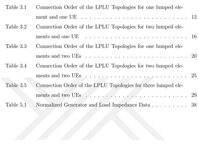
LIST OF TABLES

Table 3.1 Connection Order of the LPLU Topologies for one lumped ele-ment and one UE . . . 13 Table 3.2 Connection Order of the LPLU Topologies for two lumped

ele-ments and one UE . . . 16 Table 3.3 Connection Order of the LPLU Topologies for one lumped

ele-ments and two UEs . . . 20 Table 3.4 Connection Order of the LPLU Topologies for two lumped

ele-ments and two UEs . . . 25 Table 3.5 Connection Order of the LPLU Topologies for three lumped

ele-ments and two UEs . . . 29 Table 5.1 Normalized Generator and Load Impedance Data . . . 38

(14)

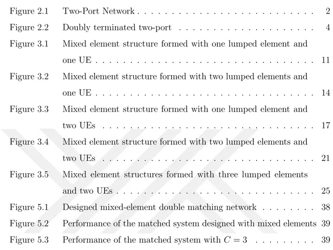
LIST OF FIGURES

Figure 2.1 Two-Port Network . . . 2 Figure 2.2 Doubly terminated two-port . . . 4 Figure 3.1 Mixed element structure formed with one lumped element and

one UE . . . 11 Figure 3.2 Mixed element structure formed with two lumped elements and

one UE . . . 14 Figure 3.3 Mixed element structure formed with one lumped element and

two UEs . . . 17 Figure 3.4 Mixed element structure formed with two lumped elements and

two UEs . . . 21 Figure 3.5 Mixed element structures formed with three lumped elements

and two UEs . . . 25 Figure 5.1 Designed mixed-element double matching network . . . 38 Figure 5.2 Performance of the matched system designed with mixed elements 39 Figure 5.3 Performance of the matched system with C = 3 . . . 39

(15)

1. INTRODUCTION

There is a significant advantage of microwave circuits according to univariate struc-tures of mixed-element, two-variable strucstruc-tures. The analytical solution of the filters having a mixed element structure and the broadband matching problem is not fully achieved. There is a need for defining mixed-element structures in using two-variable (rational form) functions. One of the methods to describe mixed lumped and dis-tributed element two-port networks is to use two-variable scattering equations.

Since these networks have two different kinds of elements, their network functions can be defined by using two variables; p = σ + jw (the usual complex frequency vari-able) for lumped elements and λ = tanh(pτ ) (the Richard varivari-able) for distributed elements, where τ is the equal delay length of distributed elements (S¸eng¨ul,2018).

In the earlier studies, since there is a hyperbolic dependence between p and λ tran-scendental functions were used to express these kinds of network functions. But then p and λ were assumed as independent variables, the network functions with two variables were used to describe two-port networks with mixed elements.

Eventough there are lots of studies in the literature about mixed element networks, a general analytic procedure to solve transcendental or multivariable approximation problems to design mixed element networks does not exist. But to describe lossless two-ports with mixed elements, there is a semi-analytic technique.

In this approach, two-variable scattering functions are used. But it is applicable for the restricted circuit topologies Inductor-Capacitor ladders cascaded with commen-surate transmission lines (Unit Elements, UEs).

(16)

In this thesis, the complete and explicit equations are derived for lossless low-pass mixed-element topologies, up to 4 elements, without any restrictions. The obtained results were compared with the literature.

(17)

2. PROPERTIES OF LOSSLESS TWO PORTS

This chapter contains about basic definitions of transmission lines and scattering parameter and matrix and canonical representation of them. Also fundamental properties of lossless lumped and distributed networks are summarized.

2.1 Defining the lossless two-port with scattering parameters

The behavior of lossless two-port circuits can be defined via matrices such as admit-tance, impedance and chain matrix. However, these matrices are defined for short or open circuit termination status. Using the concept of power in microwave circuit theory is more suitable than current or voltage concept. The scattering matrix is a very useful method to examine the power transfer characteristics of a circuit. Let us examine the scattering matrix properties and basic definitions of the two-port networks (Aksen,1994).

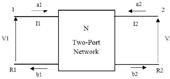
Figure 2.1 Two-Port Network Scattering variables can be defined as follows ;

(18)

ai = Vi+ RiIi 2√Ri (2.1) bi = Vi− RiIi 2√Ri (2.2) ai and bi variables are linear function of voltage and current variables defined to the

same port (Vi,Ii). Normalized input wave is indicated by ai, normalized reflected

wave is indicated by bi. (2.1) and (2.2) can be written as inverse relationship function

as seen below equations :

Vi = (ai+ bi). p Ri (2.3) Ii = (ai− bi) √ Ri (2.4) Scattering matrix of two ports (N) is as follows :

b = S.a b =   b1 b2   a =   a1 a2   S =   S11 S12 S21 S22   (2.5)

Elements of the S matrix are called scattering parameters.The following statements can be taken from the definitions in (2.5) for the physical interpretation of the scattering parameters; S11 = b1 a1 (a2)=0 S12 = b1 a2 (a1)=0 S21= b2 a1 (a2)=0 S22 = b2 a2 (a1)=0 (2.6) (ai = 0) condition shows that the termination resistance of the port ”i” is equal to

the reference normalization value Ri of the same port. S11 and S22 show input and

output reflectance coefficients of the two-port. S21 and S12 show the forward and

reverse transmission coefficients.

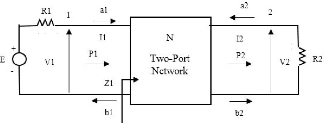
The meaning of the input reflection coefficient S11 can be found from (2.6).Z1 is the

input impedance of the two- port in figure 2.2 and current-voltage relationship for the first port is V1=Z1.I1 When terminating condition a2=0 is used ;

S11=

Z1− R1

Z1+ R1

(19)

Figure 2.2 Doubly terminated two-port

(2.7) can be found.It shows the relationship between the input impedance and the input reflection of the two-port. A similar relationship can be found for the forward transmission coefficient (S21). S21 = 2 r R1 R2 .V2 E. (2.8)

2.2 Relationship between scattering parameters and power

Scattering parameters are useful to identify power transfer from source to load in losslessness two-port. Complex power in the first and second port will be as follows,

Wi = Vi(jw)Ii(jw) (i = 1, 2) (2.9)

If equations (2.3) and (2.4) are substituted in (2.8) and the real part is taken then the entering real power is found as ;

Pi = |ai|2− |bi|2 (i = 1, 2) (2.10)

The net real power of the two- port is equal to the difference between the entering power and reflected power.

Pd= 2 X i=1 ai.ai∗− 2 X i=1 bi.bi∗ (2.11)

PA is the power given to the circuit from excitation source in 1th port and PB is

power distributed to 2nd _port.

PA= |E|2 4R1 PB = |V2|2 R2 (2.12)

(20)

After squaring the forward transmission coefficient (S21) and doing algebraic

calcu-lations, transfered power can be shown below : |S21|2 =

PB

PA

(2.13) and the distributed power from source is,

PA = |a1| =

|E|2

4R1

(2.14)

If the equations (2.5) and (2.10) combined and solved, expended power of two ports can be shown scattering parameters as below,

Pd= a∗T.(I − S∗TS).a (2.15)

I represent unit matrix and ∗T is transpose of a matrix.

2.3 Scattering Transfer Matrix

Scattering parameter (Fettweis, 1982) for the explanations of power transfer is prac-tical and useful tool for networks working at high frequencies. This method is used for finite values at output and input of the network. The tools use open circuits to find values of voltage and current of the network. Another difference between scattering parameter and others are structure of values in networks. In scattering parameters, the waves of voltage and current are utilized to calculate the efficiency of the network.

The waves are used to form for scattering parameters. The parameters a and b are used for the definition of the scattering parameters. Scattering parameters are the values of the scattering matrix of two port network as given below :

  b1 a1  = T   a2 b2  , T =   T11 T12 T21 T22   (2.16)

T parameter relationship between scattering parameter can be defined as; T11 = − det(S) S21 , T21 = − S22 S21 , T12 = − S11 S21 , T22 = − 1 S21 , (2.17)

(21)

det(S) represent determinant of transfer scattering matrix and reciprocal scattering matrix means that if S12=S21, detarminant of T will be det(T)=1.

2.4 Canonic Representation of Scattering Transfer Matrix

Representation of scattering matrix in canonic polynomials (f,g and h) is published in the literature. The canonic forms of the scattering matrix and scattering transfer matrix are shown in below:

S = 1 g   h σf∗ f −σh∗  , T = 1 f   σg∗ h σh∗ g   (2.18)

S is representation of the scattering matrix and T is representation of scattering transfer matrix. In addition, canonic polynomials have some properties. Firstly,the polynomial f = f (p), g = g(p), and h = h(p) are real and they are in the complex frequency p. g is the strictly Hurwitz polynomial means that if a single variable real polynomial has no zero in the right half plane, it is called the Hurwitz polynomial and in addition if there is no zero on the imaginary axis, it is the strictly Hurwitz polynomial. Then f,g and h polynomials have the following relation :

gg∗ = hh∗+ f f∗. (2.19)

f is a polynomial whose highest coefficient is equal to 1.Also, it is a monic.σ is a constant form of unimodular. (σ = +/ − 1) If two-port has reciprocity property,the polynomial of f can be odd or even. Then if the σ = −1 polynomial of f is odd. If the σ = +1 polynomial of f is even. Therefore, σ = f∗/f = +/ − 1 can be written

in the equation,if two-port has reciprocity property then,

gg∗ = hh∗+ σf2. (2.20)

From (2.19), the following relation are also valid,

|g| ≥ |h| , |g| ≥ |f | , (2.21)

As mentioned above, it can imply follow degree relations, and ”deg” is representation of degree of a polynomial.

(22)

The difference between deg(g) and deg(f) shows the number of transmission zeros at infinity and deg(g) refers to the degree of the lossless two-port.

(23)

3. TWO-VARIABLE CHARACTERIZATION OF MIXED

ELEMENT STRUCTURES

Two-variable polynomials g, h, f, the scattering parameters for a two-port with mixed lumped and distributed elements can be shown as follows (Aksen,1994) where |µ| = 1 is a constant : S(p, λ) =   S11(p, λ) S12(p, λ) S21(p, λ) S22(p, λ)  = 1 g(p, λ)   h(p, λ) µf (−p, −λ) h(p, λ) −µh(p, λ)   (3.1)

In above equation, p = σ + jw and λ = Σ + jΩ represent the Richards variable with transmission lines and the complex frequency related with lumped elements.

(np+ nλ)th shows the degree of the scattering Hurwitz polynomial g(p, λ) with real

coefficients. And it can be shown as g(p, λ) = PTΛgλ = λTΛTgP can be shown as

below : Λg =            g00 g01 g02 ... g0nλ g10 g11 g12 ... g1nλ g20 g21 g22 ... g2nλ ... ... ... ... g3nλ gnp0 ... ... ... gnpnλ            (3.2) PT =h1 p p2 _{... p}np i (3.3) λT =h1 λ λ2 _{... λ}nλ i (3.4)

(24)

can be shown as h(p, λ) = PTΛhλ = λTΛThP can be shown as below : Λh =            h00 h01 h02 ... h0nλ h10 g11 h12 ... h1nλ h20 g21 h22 ... h2nλ ... ... ... ... h3nλ hnp0 ... ... ... hnpnλ            (3.5)

f (p, λ) is a real polynomial and it can be shown according to the tranmission zeros of two-port as can be written as f (p, λ) = fL(p)fD(λ). and fL(p) and fD(λ) can

be constructed by means of the transmission zeros of the transmission zeros of the lumped and distributed elements.If the two-port network is lossless, the relation can be written as S(p, λ)ST_{(−p, −λ) = I and I represents the identify matrix.}

If (3.1) is substituted in S(p, λ)ST(−p, −λ) = I, the following can be found G(p, λ) = g(−p, −λ)g(p, λ) = h(−p, −λ)h(p, λ) + f (−p, −λ)f (p, λ). And this equation have to factorized explicity in designin lossless two-port with mixed elements. And if the coefficients of the similar powers of the complex frequency variable, the following equations can be set and it called as fundamental equation set (FES) is can be written : g0,k+2 k−1 X l=0 (−1)k−1g0,lg0,2k−l= h20,k+f 2 0,k+2 k−1 X l=0 (−1)k−1(h0,lh0,2k−1+f0,lf0,2k−l) (3.6) for k = 0, 1, ..., nλ i X j=0 k X l=0 (−1)i−j−lgj,lgi−j,2k−1−l = i X j=0 k X l=0

(−1)i−j−l(hj,lhi−j,2k−1−l+ fj,lfi−j,2k−1−l)

(3.7) for i = 1, 3, ..., 2np− 1 , k = 0, 1, ..., nλ i X j=0 (−1)i−j(gj,kgi−j,k+ 2 k−1 X l=0 (−1)k−lgj,lgi−j,2k−l) (3.8) = i X j=0

(−1)i−j(hj,khi−j,k+ fj,kfi−j,k+ 2 k−1

X

l=0

(25)

for i = 2, 4, ..., 2np− 2 , k = 0, 1, ..., nλ g_n2_p_,k+ k−1 X l=0 (−1)k−lgnp,lgnp,2k−l = h 2 np,k+ f 2 np,k+ k−1 X l=0 (−1)k−l(hnp,lhnp,2k−l+ fnp,lfnp,2k−l) (3.10) k = 0, 1, ..., nλ

3.1 Explicit Formulas for Low-Order Mixed-Element Structures

In the literature, low-pass ladders connected (LPLU) structure which has fundamen-tal equation set (FES) is formed by using by (Sertba¸s A,2001) and (Sertba¸s A,1997). For a transformerless design, it is solved algebraically for the unknown coefficients. In this design, coefficient of h00is restrictred as equal 0 and the explicit relations for

the entries of Λh and Λg matrices up to total degree n = np + nλ = 5 are found in

(Aksen A, Yarman 2001). Otherwise, g10 equation depends on g20 and g20 equation

depends on g10for n = 5 in (Aksen A, Yarman 2001). But in this thesis, the explicit

coefficient relations are obtained algebraically and will be given from n = 2 to n = 4 without any restrictions.

The following procedure will be followed for n = 5; If h(p, 0) is initialized and f (p, 0) is formed via f (p, λ) = pk_(1−λ2₎nλ/2_{then the strictly Hurwitz polynomial g(p, 0) can}

be calculated via G(p, λ) = g(−p, −λ)g(p, λ) = h(−p, −λ)h(p, λ) + f (−p, −λ)f (p, λ)

In the same way, if h(0, λ) is initialized then f (0, λ) is formed via f (p, λ) = pk(1 − λ2₎nλ/2 _{and the strictly Hurwitz Polynomial g(0, λ) can be found via G(p, λ) =}

g(−p, −λ)g(p, λ) = h(−p, −λ)h(p, λ) + f (−p, −λ)f (p, λ). After that, fundamental equation set is solved algebraically for the remaining unknown coefficients of Λh and

Λg matrices without any restrictions, the explicit equations for n = 5 ≥ np+ nλ will

(26)

3.1.1 Mixed element structure formed with one lumped element and one UE

The network that shown as below has one lumped element (np = 1) and one unit

element (nλ = 1).

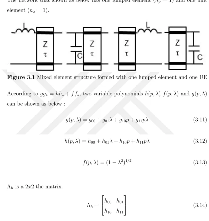
Figure 3.1 Mixed element structure formed with one lumped element and one UE

According to gg∗ = hh∗+ f f∗, two variable polynomials h(p, λ) f (p, λ) and g(p, λ)

can be shown as below :

g(p, λ) = g00+ g01λ + g10p + g11pλ (3.11) h(p, λ) = h00+ h01λ + h10p + h11pλ (3.12) f (p, λ) = (1 − λ2)1/2 (3.13) Λh is a 2x2 the matrix. Λh =   h00 h01 h10 h11   (3.14)

First column coefficients describe the lumped element section and the first row coefficients describe the distributed element section.

Λg is a 2x2 the matrix. Λg =   g00 g01 g10 g11   (3.15)

(27)

The main goal is that G and H polynomials’ coefficients can be calculated from algorithm formed by using Matlab. From the equation G(p, λ) = g(−p, −λ)g(p, λ) = h(−p, −λ)h(p, λ) + f (−p, −λ)f (p, λ), and g(−p, −λ)g(p, λ) the following equation will be obtained as follows, (g00+ g01λ + g10p + g11pλ)(g00− g01λ − g10p + g11pλ) =

(h00+ h01λ + h10p + h11pλ)(h00− h01λ − h10p + h11pλ) + (1 − λ2)1/2(1 − λ2)1/2).

If the coefficients of the respective degrees are equal, the following equation set is obtained. With the help of these equations unknown coefficients can be calculated.

g002− h002 = 1 (3.16)

g012− h012 = 1 (3.17)

g00g11− g01g10− h00h11+ h01h10= 0 (3.18)

g102− h102 = 0 (3.19)

g112− h112 = 0 (3.20)

The unknown cofficients will be calculated with above equations. From the equation (3.6)

g00 =

p

1 + h002 (3.21)

From the equation (3.7)

g01 =

p

1 + h012 (3.22)

g11 =

g01g10− h01h10

g00− µ2h00

(28)

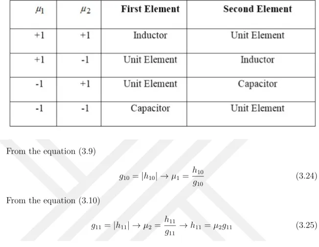
Table 3.1 Connection Order of the LPLU Topologies for one lumped element and one UE

g10= |h10| → µ1 =

h10

g10

(3.24) From the equation (3.10)

g11 = |h11| → µ2 =

h11

g11

→ h11 = µ2g11 (3.25)

3.1.2 Mixed element structure formed with two lumped elements and one UE

The network that shown as below has two lumped elements (np = 2) and one unit

element (nλ = 1).

Λh is a 3x2 matrix and h00,h01, h10, h20 are independent coefficients and h21 = 0.

Λh =      h00 h01 h10 h11 h20 0      (3.26)

(29)

Figure 3.2 Mixed element structure formed with two lumped elements and one UE Λg is a 3x2 matrix and g21= 0. Λg =      g00 g01 g10 g11 g20 0      (3.27)

g002− h002 = 1 (3.28)

g012− h012 = 1 (3.29)

(30)

g102− h102− 2(g00g20− h00h20) = 0 (3.31)

g112 − h112+ 2(g01g21− h01h21) = 0 (3.32)

g11g20− g10g21− h11h20+ h10h21= 0 (3.33)

g202− h202 = 0 (3.34)

g212− h212 = 0 (3.35)

g00 =

p

1 + h002 (3.36)

g01 =

p

1 + h012 (3.37)

g00g11− g01g10− h00h11+ h01h10= 0 (3.38) g00g11= g01g10+ h00h11− h01h10 (3.39) g11 = g01g10+ h00h11− h01h10 g00 (3.40) From the equation (3.21)

g102− h102− 2(g00g20− h00h20) = 0 (3.41)

g10 =

q

h102+ 2(g00g20− h00h20 (3.42)

g11= |h11| → µ2 =

h11

g11

(31)

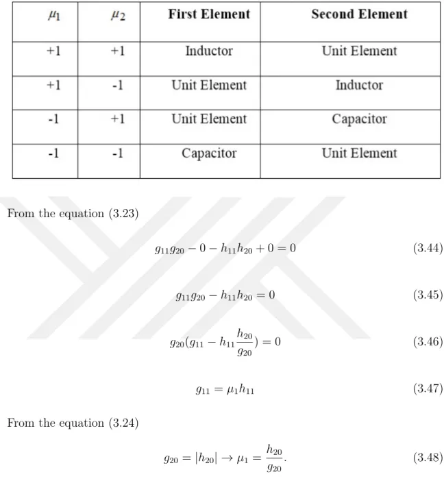
Table 3.2 Connection Order of the LPLU Topologies for two lumped elements and one UE

g11g20− 0 − h11h20+ 0 = 0 (3.44) g11g20− h11h20= 0 (3.45) g20(g11− h11 h20 g20 ) = 0 (3.46) g11= µ1h11 (3.47)

g20 = |h20| → µ1 =

h20

g20

. (3.48)

3.1.3 Mixed element structure formed with one lumped element and two UEs

The network that shown as below has one lumped element (np = 1) and two unit

elements (nλ = 2).

(32)

Figure 3.3 Mixed element structure formed with one lumped element and two UEs Λh =   h00 h01 h02 h10 h11 h12   (3.49)

Λg is a 2x3 matrix. Λh =   g00 g01 g02 g10 g11 g12   (3.50)

(33)

g₀₁2 − h2₀₁− 2(g00g02− h00h02) = 2 (3.52) g00g11− g01g10− h00h11+ h01h10= 0 (3.53) g102− h102 = 0 (3.54) g₁₁2 − h2 11− 2(g10g12− h10h12) = 0 (3.55) g11g02− g01g12− h11h02+ h01h12= 0 (3.56) g022− h022 = 1 (3.57) g122− h122 = 0 (3.58)

g00 =

p

1 + h002 (3.59)

g02 =

p

1 + h022 (3.60)

g₀₁2 − h2 01− 2(g00g02− h00h02) = 2 (3.61) g01 = q 2 + h2 01+ 2(g00g02− h00h02) (3.62)

g10 = |h10| → µ1 =

h10

g10

. (3.63)

g12 = |h12| → µ2 =

h12

g12

(34)

From the equation (3.46) g11g02− h11h02= g01g12− h01h12 (3.65) g11g02− h11h02= g12(g01− h01h12 g12 (3.66) g11g02− h11h02= g12(g01− h01µ2) (3.67) g12= g11g02− h11h02 α where α = g01− h01µ2 (3.68)

From the equation (3.45) if put the g12 and h12 in the equation

g₁₁2 − h2 11= 2(g10g12− h10h12) (3.69) g₁₁2 − h2 11= 2( g10g11g02 α − g10h11h02 α − h10g11µ2g02 α + h10h11µ2h02 α ) (3.70) g₁₁2 − h2₁₁= 2[g11( g10g02 α − h10µ2g02 α ) − h11( g10h02 α + h10µ2h02 α )] (3.71) g₁₁2 − h2 11= 2[g11( g02 α (g10− h10µ2)) − h11( h02 α (g10− h10µ2))] (3.72) g2₁₁− h2 11 = 2[g11(g02 β α) − h11(h02 β α)] (3.73) g2₁₁− h2 11 = g11 2g02β α − h11 2h02β α ) (3.74) Where β = g10− h10µ2 and α = g01− h01µ2, g11 = 2g02β α (3.75) h11 = 2h02β α (3.76)

(35)

Table 3.3 Connection Order of the LPLU Topologies for one lumped elements and two UEs

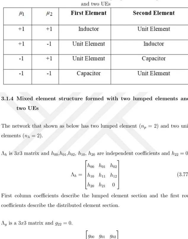
3.1.4 Mixed element structure formed with two lumped elements and two UEs

The network that shown as below has two lumped element (np = 2) and two unit

elements (nλ = 2).

Λh is 3x3 matrix and h00,h01,h02, h10, h20 are independent coefficients and h22 = 0.

Λh =      h00 h01 h02 h10 h11 h12 h20 h21 0      (3.77)

Λg is a 3x3 matrix and g22= 0. Λg =      g00 g01 g02 g10 g11 g12 g20 g21 0      (3.78)

(36)

Figure 3.4 Mixed element structure formed with two lumped elements and two UEs

algorithm formed by using Matlab. From the equation G(p, λ) = g(−p, −λ)g(p, λ) = h(−p, −λ)h(p, λ) + f (−p, −λ)f (p, λ), and g(−p, −λ)g(p, λ) the following equation will be obtained as follows, (g00+ g01λ + g10p + g11pλ)(g00− g01λ − g10p + g11pλ) =

g002− h002 = 1 (3.79) g₀₁2 − h2₀₁− 2(g00g02− h00h02) = 2 (3.80) g00g11− g01g10− h00h11+ h01h10= 0 (3.81) g102− h102− 2(g00g20− h00h20) = 0 (3.82) g112− h112− 2(g01g21− g02g20+ g10g12− g00g22− h01h21− h02h20− h10h12+ h00h22) = 0 (3.83)

(37)

g11g02− g01g12− h11h02+ h01h12= 0 (3.84) g022− h022 = 1 (3.85) g122− h122− 2(g02g22− h02h22) = 0 (3.86) g11g20− g10g21− h11h20+ h10h21= 0 (3.87) g11g22− g12g21− h11h22+ h12h21= 0 (3.88) g202− h202 = 0 (3.89) g212 − h212+ 2(h20h22− g20g22) = 0 (3.90) g222− h222 = 0 (3.91)

g00 =

p

1 + h002 (3.92)

g02 =

p

1 + h022 (3.93)

From the equation (3.70) g01 =

q

2 + 2(g00g02− h00h02+ h201) (3.94)

g20= |h20| → µ1 =

h20

g20

(3.95) From the equation (3.80)

g21 = |h21| → µ2 =

h21

g21

(38)

g12 = |h12| → µ3 =

h12

g12

→ h12 = µ3g12 (3.97)

−g12g21+ h12h21= 0 (3.98) h21 g21 = µ2 = g12 h12 = µ3 → µ2 = µ3 (3.99)

g11g02− h11h02= −h01h12+ g01g12 (3.100)

g11g02− h11h02 = g12(g01− h01

h12

g12

) (3.101)

and (3.87) equation shows that h12

g12 equal µ2 so that,

g12 =

g11g02− h11h02

α (3.102)

where α = g01− h01µ2.

g11g20− h11h20= g10g21− h10h21 (3.103) g11g20− h11h20= g21(g10− µ2h10) (3.104) g21 = g11g20− h11h20 β (3.105) where β = g10− µ2h10.

g00g11− g01g10− h00h11+ h01h10= 0 (3.106)

(39)

g11 = g01g10+ h00h11− h01h10 g00 (3.108) g11 = h00h11+ γ g00 (3.109) where γ = g01g10− h01h10.

g112− h112− 2(g01g21− g02g20+ g10g12− g00g22− h01h21− h02h20− h10h12+ h00h22= 0 (3.110) h11= h20α_β + h02β_α − h_g₀₀00(g20α_β + g02β_α) + h_g002 00γ 1 −h200 g2 00 (3.111) where γ = g01g10− h01h10.

g102− h102 = 2(g00g20− h00h20) (3.112) g₁₀2 = h2₁₀+ 2(g00g20− h00h20) (3.113) g10 = q h2 10+ 2(g00g20− h00h20) (3.114)

3.1.5 Mixed element structure formed with three lumped elements and two UEs

The network that shown as below has three lumped element (Np = 3) and two unit

elements (Nλ = 2).

Λh is a 4x3 matrix and h00,h01,h02, h10, h20 and h30 are independent coefficients and

h22 = h31 = h32= 0 Λh =         h00 h01 h02 h10 h11 h12 h20 h21 0 h30 0 0         (3.115)

(40)

Table 3.4 Connection Order of the LPLU Topologies for two lumped elements and two UEs

Figure 3.5 Mixed element structures formed with three lumped elements and two UEs

Λg is a 4x3 matrix and g22= g31 = g32= 0. Λg =         g00 g01 g02 g10 g11 g12 g20 g21 0 g30 0 0         (3.116)

The main goal is that G and H polynomials’ coefficients can be calculated from algorithm formed by using Matlab. From the equation G(p, λ) = g(−p, −λ)g(p, λ) = h(−p, −λ)h(p, λ) + f (−p, −λ)f (p, λ), and g(−p, −λ)g(p, λ) the following equation

(41)

will be obtained as follows, (g00+ g01λ + g10p + g11pλ)(g00− g01λ − g10p + g11pλ) =

g002− h002 = 1 (3.117) g₀₁2 − h2 01− 2(g00g02− h00h02) = 2 (3.118) g00g11− g01g10− h00h11+ h01h10= 0 (3.119) g102− h102− 2(g00g20− h00h20) = 0 (3.120) g112− h112− 2(g01g21− g02g20+ g10g12− g00g22− h01h21− h02h20− h10h12+ h00h22) = 0 (3.121) g11g02− g01g12− h11h02+ h01h12= 0 (3.122) g022− h022 = 1 (3.123) g122− h122− 2(g02g22− h02h22) = 0 (3.124) g11g20− g10g21− g01g30+ g00g31− h11h20+ h10h21+ h01h30− h00h31 = 0 (3.125) g11g22− g12g21− g01g32+ g02g31− h11h22+ h12h21+ h01h32− h02h31 = 0 (3.126) g202− h202− 2(g10g30− h10h30) = 0 (3.127) g212− h212− 2(g10g32+ g12g30− g20g22+ h10h32+ h12h30− h20h22) = 0 (3.128)

(42)

g222− h222− 2(g12g32− h12h32) = 0 (3.129) g20g31− g21g30− h20h31+ h21h30= 0 (3.130) g22g31− g21g32− h22h31+ h21h32= 0 (3.131) g302− h302 = 0 (3.132) g312− h312− 2(g30g32− h30h32) = 0 (3.133) g322− h322 = 0 (3.134)

g00 =

p

1 + h002 (3.135)

q 2 + h2

01+ 2(g00g02− h00h02) (3.136)

g00g11− g01g10− h00h11+ h01h10= 0 (3.137) g00g11= g01g10+ h00h11− h01h10 (3.138) g11 = g01g10+ h00h11− h01h10 g00 (3.139) g11 = h00h11+ γ g00 (3.140) where γ = g01g10− h01h10.

(43)

g₁₀2 = h2₁₀+ 2(g00g20− h00h20) (3.142)

g10 =

q h2

10+ 2(g00g20− h00h20) (3.143)

g11g02− h11h02= −h01h12+ g01g12 (3.144)

g11g02− h11h02 = g12(g01− h01

h12

g12

) (3.145)

and (3.116) equation shows that h12

g12 equals µ2 so that,

g12 =

g11g02− h11h02

α (3.146)

where α = g01− h01µ2.

g02 =

p

1 + h022 (3.147)

g11g20− h11h20= g10g21− h10h21 (3.148)

and (3.116) equation shows that g21

h21 equals µ2 so that, g11g20− h11h20= g21(g10− µ2h10) (3.149) g21 = g11g20− h11h20 β (3.150) where β = g10− µ2h10.

g12g21= h12h21 (3.151) h12 g12 = g12 h12 = g21 h21 = h21 g21 = µ2 (3.152)

(44)

Table 3.5 Connection Order of the LPLU Topologies for three lumped elements and two UEs

q h2

20+ 2(g10g30− h10h30) (3.153)

g21g30− h21h30= 0 (3.154)

g30(g21− h21

h30

g30

) = 0 (3.155)

The connection order of the LPLU topologies for three lumped elements and two UEs table will be given below :

g112− h112− 2(g01g21− g02g20+ g10g12− g00g22− h01h21− h02h20− h10h12+ h00h22) = 0 (3.156) h11= h20α_β + h02β_α − h_g00 00(g20 α β + g02 β α) + h00 g2 00γ 1 −h200 g2 00 (3.157) where γ = g01g10− h01h10.

g30= |h30| → µ3 =

h30

g30

(45)

4. BROADBAND MATCHING METHODS

4.1 Real Frequency Matching with Scattering Parameters

The matching problem is formulated by scattering parameters of the lossless equal-izer network. That frequency scattering approach is Simplified Real Frequency Tech-nique (SRFT) (Yarman, 1985). Matching network which is a lossless identified with the scattering parameters are formed with canonic polynomials f,g,h.

The canonic polynomials are represented with Belevitch representation. S11= h(p) g(p) S12= σ f (−p) g(p) S21 = f (p) g(p) S22= −σ h(−p) g(p) σ = f (p) f (−p) (4.1) In the above equations, σ is a constant (+1 or -1), f (p) is a real monic polynomial and g(p) is a Hurtwitz polynomial. When the two port N is reciprocal, then f is either odd or even.

Relation in terms of degree between f (p), g(p) and h(p) polynomials is that g(p) polynomial can be bigger or equal than degree of f (p) and h(p) polynomials.

The relation f (p), g(p) and h(p) can be seen below:

g(p)g(−p) = h(p)h(−p) + f (p)f (−p) (4.2)

f (p) and h(p) polynomials are the parameters of Hurwitz polynomial g(p).The net-work’s definitions can be shown with f (p) and h(p) polynomials. f (p) polynomial is the zeros of transmission of the matching two port network and it is depending on the distributed elements numbers and chosed lumped elements by the designer.

(46)

determined. Also, f (p) will be calculated with degree of n because of those selections. Then, the cofficients of h(p) can be initialized and g(p) can be calculated via (4.2). Polynomials’ calculations can be used to calculate the value of scattering parameters in the equation (4.1).

Transducer power gain can be shown as below : T P G(w) = (1 − |Sin|

2_)|S

21|2(1 − |SL|2)

|1 − S11Sin|2|1 − SoutSL|2

(4.3)

Sin represent of input reflection coefficient and it is terminated ZL. SL shows the

load reflection coefficient. Sout represents the output reflection cofficient and also

it is terminated Zin.S22 shows the reflection coeffient of port 2 and S11 shows the

reflection coeffient of port 1.

For the calculations of the transducer power gain, the real coefficients are needed to be initialized (S¸eng¨ul and C¸ akmak,2018). Then, f (p)’s polynomial form should be selected and the degree have to equal or less than g(p). After that, calculating gg∗ via f f ∗+hh∗ and finding roots of G(p) = gg∗. With the known parameters of f (p) and h(p) polynomials, the scattering parameters can be calculated via (4.1) and reflection coefficients can be calculated to find TPG in the equation (4.3).

4.2 Parametric Representation of Brune Functions

Brune functions which the method is proposed for single matching problems are de-velop by Fettweis (Fettweis, 1979) and it is depended the parametric representation of the positive real impedance Zout(p) of a lossless network. Zout is the positive real

impedance. And it is identification of impedance while looking from the 2.port to the generator. It can be solved in a partial fraction expansion. Furthermore, the parameters can be used to identify the poles of Zout to optimizate gain performance

of the system for matching load network.

(47)

that it shows minimum reactance function so it is identified from its even part. That means, Zout equals Zout(p) = odd(p) + even(p) and e(p) equals Rout(p). The equal

equation shows that Rout(p) is Hilbert transformation of the Zout(p) (S¸eng¨ul and

C¸ akmak,2018).

The positive real impedance function Zout(p) as shown below :

Zout= C0+ k X i=1 Ci p − pi (4.4)

C0 represents real constant. Complex constant is p which is the distinct poles of

Zout with Re(pi) < 0.

Zout(Even) =

Zout(p) + Zout(p)

2 =

f (p)f (−p)

n(p)n(−p) (4.5)

f (p) and Zout(p) represent real polynomial and n(p) is the Hurtwitz denominator of

these polynomials. In lossless reciprocal two-ports, it can be odd or even polynomial. Whether Zoutis a minimum reactance function, the poles are located in the left half

of the complex p plane.

d(p) which is the Hurtwitz denominator polynomial can be shown as below and Dk

represents non-zero conctant :

d(p) = Dk k

Y

i=1

(p − pi) (4.6)

If combine the equations (4.5) and (4.6), getting the below formula :

C0+ k X i=1 Ci p − pi = f (p)f (−p) n(p)n(−p) (4.7)

If combine the equations (4.6) and (4.7), getting the below formula, Ci = − f (pi)f (−pi) p1D2k Qk i=1(p 2 i − p21) (4.8)

(48)

When f (p) polynomial’s degree is smaller than k, C0 equals to 0. When f (p)

poly-nomial’s degree equals to k, C0 equals _D12 k

. In the equation (4.28), Zout can be shown

depends on f (p) and d(p).

The monic polynomial can be represented as below :

f (p) = pk1 k2

X

i=0

bip2i (4.9)

If the k2 and k1 show nonnegative integers, bi will be equaled an arbitrary real

coefficients. When f (p) polynomial’s zeros are located on the real frequency axis of the p plane, and f (p) can be represented as:

f (p) = pk1 k2 Y i=0 (p2− a2 i) (4.10)

When the number of poles equals odd, the poles should be chosen real. Otherwise, the number of poles are even, the poles can be thought as conjugate pairs.

As mentioned above, the output impedance parameters can be shown as :

Rout = − k X i=1 C0+ Cipi w2_{+ p}2 i (4.11) Xout(w) = −w k X i=1 Ci w2 _{+ p}2 i (4.12)

4.3 Line Segment Technique for a Single Matching Problem

The network has a resistance at input port and a complex load at output port (S¸eng¨ul and C¸ akmak,2018). To calculate a transducer power gain, the equalizer network have to be calculated.

ZL represents the load impedance and Zout represents output impedance as shown

(49)

ZL(jw) = RL(w) + jXL (4.13)

Zout(jw) = Rout+ jXout (4.14)

Sout =

Zout(jw) − ZL(jw)

(4.15)

T P G(w) = 1 − |Sout|2 (4.16)

TPG can be obtained with the imaginary and real parts of load ZL(jw) and Zout(jw)

is the output impedance. And transducer power gain can be written as ;

T P G(w) = 4RintRin

(Rint+ Rin)2+ (Xint+ Xin)2

= 4RoutRL

(Rout+ RL)2+ (Xout+ XL)2

(4.17)

Rout and Xout are parameters of output impedances and they can be calculated for

maximum transducer power gain. The real frequency approach (Carlin and Yarman, 1983) can be showed to get these Zout value.

Zout has the unknown real parts and it represented a number of line segments Rout

(Carlin, 1977). Rout = k0+ n X j=1 bj(w)kJ (4.18)

bj(w) represents identification in Routvia to the sampling frequency (wj, j = 1, 2, 3, 4, ...n).

Output impedance has the imaginary part and it can be calculated with Hilbert transformation (Carlin, 1977). Xout can be identified using the same line segments

representation as shown below :

Xout = n

X

j=1

cj(w)kJ (4.19)

And then cj(w) can be calculated via Hilberts transformation technique as show

below :

cj(w) =

1 π(wj− wj−1)

(50)

I(w) can be calculated as below : I(w) = Z wj wj−1 In|y + w y − w|dy (4.21)

The tranducer power gain equation (4.17) can be found after the calculation un-known output impedance. To minimize the difference between the actual power gain and the target, the least square method can be used as below :

E =

Nw

X

j=1

(T (wj, kj) − Td)2 (4.22)

Td represents the target value of TPG. E equals the difference of the actual and

desired one. Number of sampling frequency representing by Nw.

4.4 Direct Computational Technique for Double Matching Problems

Direct computational technique is developed by Carlin and Yarman (Carlin and Yarman, 1983). It can be used for solving double matching problems. The method includes that the real part is simplified a real even rational function with the un-known coefficients to optimize the characteristic of the gain over a specified pass-band.

The technique is included the output impedance that is unknown parameter. Trans-ducer power gain will be showed and Sin represents the complex normalized input

reflection coefficient and it can be used for transducer power gain. As follows below, Sintcan be seen and Zin represents generator impedance at port one, Zint shows the

input impedance, ZL represents the load impedance and Zout represents the output

impedance in the network.

Sint=

Zint− Zin

Zint+ Zin

(4.23) Sin which represents the reflection coefficient of the generator can be shown as :

Sin=

Zin− 1

Zin+ 1

(4.24) Sint which represents the reflection coefficient of the port one can be shown as :

Sint=

Zint− 1

Zint+ 1

(51)

TPG can be shown below in terms of Sin and Sint : T P G(w) = (1 − |Sin| 2_{)(1 − |S} int|2) |1 − SinSint|2 (4.26) The aim is that to identify Sin in terms of a function of the impedance Z2.Also, Sint

can be identified in terms of the scattering parameters as below : Sint= S11+ S2 12SL 1 − S22SL = −SLQ + S11 1 − SLS22 (4.27) where Q = S11S22− S212 . And the below equation can be found :

Q = S22 S11

= S12 S21

(4.28) Combine the equations, Sint can be represented as :

Sint = S12(SLS22∗) S21∗ (1 − SLS22) S22= Zout− 1 Zout+ 1 Zout = n d (4.29)

Thanks to the equation (4.29), the even part of the Zout can be seen as :

ev(Zout) = 1 2(Zout+ Zout∗) = n d n∗ d∗ = HH ∗ H = f ∗ d (4.30)

As mentioned above, Sint can be shown as :

Sint = H H∗ = ZL− Zout∗ ZL+ Zout (4.31) And below equation means that Zout impact to calculate the ratio of TPG with ZL

(52)

5. BROADBAND MATCHING NETWORK DESIGN

VIA EXPLICIT SOLUTIONS OF TWO VARIABLE

SCATTERING EQUATIONS

In this chapter, we will present broadband double matching network design.

5.1 Broadband Double Matching Network Design

In this example, LPLU network which has four elements is employed to match the load and generator impedances. For this LPLU network, np = 2, nλ = 2 and the

frequency band is 1 ≥ w ≥ 0. The broadband double matching network which improved (Aksen and Yarman,2001) will be compared with the low-pass mixed el-ement broadband matching network (two lumped and two unit elel-ements) has been designed by using the equations given the third part in the thesis.

τ represents the delay length which is chosen as the unknown coefficients and also the coefficicients ( h00,h01,h02,h10,h20) are chosen as the unknown coefficients. µ2

is the constat for defining as −1. Another constant µ1 will be obtained at the end

of the optimization process by using the sign of h20. If h20 is negative, µ1 equals

−1 and if h20 equals positive, µ1 equals +1. The unknown coefficients of λh and λg

matrices can be calculated by means of the explicit equations given the third part in the thesis.

The purpose is that trying an efficient network for transfer power via equalized net-work. And the network has a parallel inductor and a load capacitor. The normalized generator and load impedance datas are given below :

(53)

Table 5.1 Normalized Generator and Load Impedance Data

Figure 5.1 Designed mixed-element double matching network

Then completed the optimization process, the coefficient matrices which are showed below that completely describe the scattering parameters of the matching network under consideration are obtained :

Λk =      −0.1076 −3.4667 −2.7720 0.3723 −5.6308 −11.6498 1.1199 −8.2039 0      , Λg =      1.0058 4.3988 2.9468 1.6225 8.9814 11.6498 1.1199 8.2039 0      (5.1)

The designed network with the normalized element values and the gain performance of the system are shown below :

Proposed Values: L = 1.7916, C = 1.392, Z1 = 0.137, Z2 = 0.701, τ = 0.2 n = 0.8982

Following reference values are taken from the (Aksen and Yarman,2001). Reference Values: L = 2.126, C = 0.751, Z1 = 0.161, Z2 = 0.341, τ = 0.21

(54)

Figure 5.2 Performance of the matched system designed with mixed elements

(55)

In the design, an ideal transformer is used which simply scales current and voltage. It does not have any inductance or frequency dependency. So DC passes through like all other frequencies. Then ideally there will be a power transfer at DC. But practically a transformer will not transfer any power at DC.

If the normalized capacitor value in the load is increased to 3, then the maximum available flat gain level equals about 0.8 (Fano,1950) (Youla,1964). But the trans-ferred gain at DC will be unity. Then the gain will reduce dramatically to 0.8 levels in the passband as seen in the figure. On the other hand,a more flat trans-ducer power gain curve fluctuating around 0.8 is obtained by means of the derived equations.

There is no transformer in (Aksen and Yarman,2001) (h00 is restricted and h00

equals 0),the low pass network is designed and the generator and load resistors are equal, the transferred gain is unity at DC. After that, the gain level reduces to approximately 0.95 (Fano,1950) (Youla,1964). For the maximum available gain for the selected load is ideally close to unity,this gain drop is not noticeable.

(56)

6. CONCLUSIONS

Mixed element networks are included different elements. The network which has mixed element structures can be defined by two variables which one of them is lumped element and the other is distributed element and were assumed as indepented variables. In this thesis, the complete and explicit equations are derived for lossless low-pass mixed-element topologies, and by using the equations solved without any restrictions, a broadband matching network design was made.

Explicit design equations have been solved up to four elements for LPLU without any restrictions. In case of five-element, it is obtained that the first row and column coefficients of the two-variable polynomial g, explicit equations are found for the unknown coefficients of Λg and Λh matrices without any restrictions. Then, the

broadband matching network design was created. The results were compared with the results in the literature.

The utilization of the given explicit equations is demonstrated via a broadband double matching example. It is expected that the proposed equations will be used to design two-variable networks such as broadband matching networks, microwave amplifiers.

(57)

APPENDIX A: Matlab Codes

A.1 Matlab Codes for Main Program

c l c t i c c l e a r syms L f r

g l o b a l m2 d i s t lump w SG SL T0 ZG ZL f p mu

%∗∗∗∗∗ s o u r c e and l o a d impedance , s o u c e and %l o a d r e l e c t i o n c o e f f i c i e n t c a l c u l a t i o n ∗∗∗∗∗ w= 0 : 0 . 1 : 1 ; z=i . ∗ f r .∗2+(1/(1+ i ∗ f r ∗ 1 ) ) ; ZL=s u b s ( z , f r , w ) ; r 1 1 =1; r 3 3=i . ∗ f r . ∗ 1 ; z11=r 1 1+r 3 3 ; z11=s i m p l e ( z11 ) ; ZG=s u b s ( z11 , f r , w ) ; % ZG=o n e s ( 1 , l e n g t h (w ) ) ; SG=(ZG− 1 ) . / (ZG+ 1 ) ; SL=(ZL− 1 ) . / ( ZL+ 1 ) ; %∗∗∗∗∗∗∗∗∗∗∗∗∗∗∗∗∗∗∗∗∗∗∗∗∗∗∗∗∗∗∗∗∗∗∗∗∗∗∗∗∗∗∗∗∗∗∗∗∗∗∗∗∗∗∗∗∗

(58)

%∗∗∗∗∗ I n i t i a l v a l u e s ∗∗∗∗∗∗∗∗∗∗∗∗∗∗∗∗∗∗∗∗∗∗∗∗∗∗∗∗∗∗∗∗∗∗∗∗∗∗∗∗∗∗∗ h 0 i =[1 −1 1 ] ; %d i s t h j 0 =[−1 1 ] ; %lumped T0 = 0 . 9 9 ; %g a i n thau = 0 . 2 ; %d e l a y %∗∗∗∗∗∗∗∗∗∗∗∗∗∗∗∗∗∗∗∗∗∗∗∗∗∗∗∗∗∗∗∗∗∗∗∗∗∗∗∗∗∗∗∗∗∗∗∗∗∗∗∗∗∗∗∗∗∗ %∗∗∗∗∗ O p t i m i s a t i o n v e c t o r c o n s t r u c t i o n ∗∗∗∗∗∗∗∗∗∗∗∗∗∗∗∗∗∗∗∗∗∗∗∗∗∗∗∗ d i s t=l e n g t h ( h 0 i ) −1; lump=l e n g t h ( h j 0 ) ; d i m e n s i o n=d i s t+lump ; i f d i s t==lump

m2=i n p u t ( ’ E nte r m2 v a l u e ( + 1 / − 1 ) : ’ ) ; % ORNEK GIR end f o r a =1: d i s t +1; v ( a)= h 0 i ( a ) ; end f o r a =1: lump ; v ( d i s t +1+a)= h j 0 ( a ) ; end v ( d i m e n s i o n +2)=thau ; %∗∗∗∗∗∗∗∗∗∗∗∗∗∗∗∗∗∗∗∗∗∗∗∗∗∗∗∗∗∗∗∗∗∗∗∗∗∗∗∗∗∗∗∗∗∗∗∗∗∗∗∗∗∗∗∗ f p =(1−L ˆ 2 ) ˆ ( d i s t / 2 ) ; mu=1; %∗∗∗∗∗ o p t i m i s a t i o n p a r t ∗∗∗∗∗∗∗∗∗∗∗∗∗∗∗∗∗∗∗∗∗∗∗∗∗∗∗∗∗∗∗∗∗∗∗∗ c o n s t=l e n g t h ( v ) ; LB=[ o n e s ( 1 , c o n s t −1).∗( − I n f ) 0 . 2 ] ;

(59)

UB=o n e s ( 1 , c o n s t ) . ∗ I n f ;

OPTIONS=o p t i m s e t ( ’ MaxFunEvals ’ , 1 0 0 0 , ’ MaxIter ’ , 2 5 0 0 , ’ TolCon ’ , 1 e −32 , ’ TolX ’ , 1 e −32 , ’ TolFun ’ , 1 e −32);

v new=f m i n c o n ( @ e r r o r s r f t , v , [ ] , [ ] , [ ] , [ ] , LB , UB, [ ] , OPTIONS ) ; %∗∗∗∗∗∗∗∗∗∗∗∗∗∗∗∗∗∗∗∗∗∗∗∗∗∗∗∗∗∗∗∗∗∗∗∗∗∗∗∗∗∗∗∗∗∗∗∗∗∗∗∗∗∗∗∗∗∗ %∗∗∗∗∗ G e t t i n h 0 i , h j 0 and thau a f t e r o p t i m i s a t i o n ∗∗∗∗∗∗∗∗∗∗∗∗∗∗∗∗∗ f o r a =1: d i s t +1; h 0 i ( a)=v new ( a ) ; end ; h 0 i ; f o r a =1: lump ;

h j 0 ( a)=v new ( d i s t +1+a ) ; end ;

h j 0 ( lump+1)= h 0 i ( l e n g t h ( h 0 i ) ) ; h j 0 ;

thau=v new ( d i s t+lump + 2 ) ;

i f h j 0 (1) >0 m1=1; e l s e m1=−1; end %∗∗∗∗∗∗∗∗∗∗∗∗∗∗∗∗∗∗∗∗∗∗∗∗∗∗∗∗∗∗∗∗∗∗∗∗∗∗∗∗∗∗∗∗∗∗∗∗∗∗∗∗∗∗∗∗ %∗∗∗∗∗ C a l c u l a t i o n o f o p t i m i s e d h and g m a t r i c e s ∗∗∗∗∗∗∗∗∗∗∗∗∗∗∗∗∗∗∗ i f d i s t ==1 & lump==1; [ Ah , Ag]= hg11n ( h 0 i , hj0 , m1 , m2 , f p ) ;

(60)

e l s e i f d i s t ==1 & lump==2; m2=m1 ; [ Ah , Ag]= hg12n ( h 0 i , hj0 , m1 , m2 , f p ) ; e l s e i f d i s t ==2 & lump==1; i f m1==1 m2=−1; e l s e m2=1; end [ Ah , Ag]= hg21n ( h 0 i , hj0 , m1 , m2 , f p ) ; e l s e i f d i s t ==2 & lump==2; [ Ah , Ag]= hg22n ( h 0 i , hj0 , m1 , m2 , f p ) ; e l s e i f d i s t ==2 & lump==3; m2=m1 ; [ Ah , Ag]= hg23n ( h 0 i , hj0 , m1 , m2 , f p ) ; end Ah Ag thau %∗∗∗∗∗∗∗∗∗∗∗∗∗∗∗∗∗∗∗∗∗∗∗∗∗∗∗∗∗∗∗∗∗∗∗∗∗∗∗∗∗∗∗∗∗∗∗∗∗∗∗∗∗∗∗∗∗∗∗∗∗∗ %∗∗∗∗ C a l c u l a t i o n o f l o a d and s o u r c e impedances , % s o u r c e and l o a d r e f l e c t i o n c o e f f i c i e n t s o v e r new f r e q u e n c y r a n g e ∗∗ w= 0 : 0 . 0 1 : 2 ; ZL=s u b s ( z , f r , w ) ; ZG=s u b s ( z11 , f r , w ) ; % ZG=o n e s ( 1 , l e n g t h (w ) ) ; SG=(ZG− 1 ) . / (ZG+ 1 ) ; SL=(ZL− 1 ) . / ( ZL+ 1 ) ;

(61)

%∗∗∗∗∗∗∗∗∗∗∗∗∗∗∗∗∗∗∗∗∗∗∗∗∗∗∗∗∗∗∗∗∗∗∗∗∗∗∗∗∗∗∗∗∗∗∗∗∗∗∗∗∗∗∗∗∗∗∗∗∗∗∗

%∗∗∗∗∗ A c c o r d i n g t o o p t i m i s e d h and g m a t r i c e s , g e t t i n g t h e v a l u e s % o f h , hpara , g , g p a r a and f ∗∗∗∗∗

f o r a =1: l e n g t h (w ) ; d=i ∗ tan (w( a ) ∗ thau ) ; hv ( a ) = 0 ; f o r b=1: lump +1; f o r c =1: d i s t +1; hv ( a)=hv ( a)+Ah( b , c ) ∗ ( ( i ∗w( a ) ) ˆ ( b −1))∗( d ) ˆ ( c −1); end end end f o r a =1: l e n g t h (w ) ;

d=−i ∗ tan (w( a ) ∗ thau ) ; hpv ( a ) = 0 ; f o r b=1: lump +1; f o r c =1: d i s t +1; hpv ( a)=hpv ( a)+Ah( b , c )∗(( − i ∗w( a ) ) ˆ ( b −1))∗( d ) ˆ ( c −1); end end end f o r a =1: l e n g t h (w ) ; d=i ∗ tan (w( a ) ∗ thau ) ; gv ( a ) = 0 ;

f o r b=1: lump +1; f o r c =1: d i s t +1;

gv ( a)=gv ( a)+Ag( b , c ) ∗ ( ( i ∗w( a ) ) ˆ ( b −1))∗( d ) ˆ ( c −1); end

(62)

end end

f o r a =1: l e n g t h (w ) ;

d=−i ∗ tan (w( a ) ∗ thau ) ; gpv ( a ) = 0 ; f o r b=1: lump +1; f o r c =1: d i s t +1; gpv ( a)=gpv ( a)+Ag( b , c )∗(( − i ∗w( a ) ) ˆ ( b −1))∗( d ) ˆ ( c −1); end end end %∗∗∗∗∗∗∗∗∗∗∗∗∗∗∗∗∗∗∗∗∗∗∗∗∗∗∗∗∗∗∗∗∗∗∗∗∗∗∗∗∗∗∗∗∗∗∗∗∗∗∗∗∗∗∗∗∗∗ f v=s u b s ( f p , L , i . ∗ tan (w. ∗ thau ) ) ; f p v=c o n j ( f v ) ; %∗∗∗∗∗ C a l c u l a t i o n o f tpg o v e r t h e f r e q u e n c y r a n g e ∗∗∗∗∗∗∗∗∗∗∗∗∗∗∗∗∗ S22=−mu. ∗ hpv . / gv ; S12=mu. ∗ f p v . / gv ; S21=f v . / gv ; S11=hv . / gv ; SL=(ZL− 1 ) . / ( ZL+ 1 ) ; S1=S11+(S12 . ∗ S21 . ∗ SL ) . / ( 1 − S22 . ∗ SL ) ; Z11=(1+S1 ) . / ( 1 − S1 ) ; r 1 =(Z11−c o n j (ZG ) ) . / ( Z11+ZG ) ; SG=(ZG− 1 ) . / (ZG+ 1 ) ; S2=S22+(S12 . ∗ S21 . ∗SG) . / ( 1 − S11 . ∗SG ) ; Z22=(1+S2 ) . / ( 1 − S2 ) ;

(63)

tpg = ( 4 .∗ r e a l ( ZL ) . ∗ r e a l ( Z22 ) ) . / ( ( r e a l ( ZL)+ r e a l ( Z22 ) ) . ˆ 2 + ( imag ( ZL ) +imag ( Z22 ) ) . ˆ 2 ) ; %∗∗∗∗∗∗∗∗∗∗∗∗∗∗∗∗∗∗∗∗∗∗∗∗∗∗∗∗∗∗∗∗∗∗∗∗∗∗∗∗∗∗∗∗∗∗∗∗∗∗∗∗∗∗∗∗∗∗ %∗∗∗∗∗ P l o t t i n g t h e r e s u l t ∗∗∗∗∗ h o l d on r e n k =(round ( rand ( 3 , 1 ) ) ) ’ ; d i v =(round ( rand ( 3 , 1 ) ) ) ’ + 1 ; c o l o r =[ r e n k ( 1 ) / d i v ( 1 ) r e n k ( 2 ) / d i v ( 2 ) r e n k ( 3 ) / d i v ( 3 ) ] ; p l o t (w, T0 , ’ r ’ , w, tpg , ’ c o l o r ’ , c o l o r ) a x i s ( [ 0 2 0 1 ] ) %∗∗∗∗∗∗∗∗∗∗∗∗∗∗∗∗∗∗∗∗∗∗∗∗∗∗∗∗∗∗∗∗∗∗∗∗∗∗∗∗∗∗∗∗∗∗∗∗∗∗∗∗∗∗∗∗∗∗∗ t o c

(64)

A.2 Matlab Codes for Error Calculation

f u n c t i o n e p s= e r r o r s r f t ( v )

syms L f r

g l o b a l m2 d i s t lump w SG SL T0 ZG ZL f p mu

%∗∗∗∗∗ e r r o r sub−program ∗∗∗∗∗

%∗∗∗∗∗ c a l c u l a t i o n o f h 0 i , h j 0 and thau from o p t i m i s a t i o n v e c t o r ∗∗∗∗∗ d i m e n s i o n=d i s t+lump ; f o r a =1: d i s t +1; h 0 i ( a)=v ( a ) ; end f o r a =1: lump ; h j 0 ( a)=v ( d i s t +1+a ) ; end h j 0 ( lump+1)= h 0 i ( l e n g t h ( h 0 i ) ) ; thau=v ( d i s t+lump + 2 ) ; %∗∗∗∗∗∗∗∗∗∗∗∗∗∗∗∗∗∗∗∗∗∗∗∗∗∗∗∗∗∗∗∗∗∗∗∗∗∗∗∗∗∗∗∗∗∗∗∗∗∗∗∗∗∗∗∗∗∗ i f h j 0 (1) >0 m1=1; e l s e m1=−1; end %∗∗∗∗∗ C a l c u l a t i o n o f h and g m a t r i c e s ∗∗∗∗∗∗∗∗∗∗∗∗∗∗∗∗∗∗∗∗∗∗∗∗∗∗∗∗∗

(65)

i f d i s t ==1 & lump==1; [ Ah , Ag]= hg11n ( h 0 i , hj0 , m1 , m2 , f p ) ; e l s e i f d i s t ==1 & lump==2; m2=m1 ; [ Ah , Ag]= hg12n ( h 0 i , hj0 , m1 , m2 , f p ) ; e l s e i f d i s t ==2 & lump==1; i f m1==1 m2=−1; e l s e m2=1; end [ Ah , Ag]= hg21n ( h 0 i , hj0 , m1 , m2 , f p ) ; e l s e i f d i s t ==2 & lump==2; [ Ah , Ag]= hg22n ( h 0 i , hj0 , m1 , m2 , f p ) ; e l s e i f d i s t ==2 & lump==3; m2=m1 ; [ Ah , Ag]= hg23n ( h 0 i , hj0 , m1 , m2 , f p ) ; end %∗∗∗∗∗∗∗∗∗∗∗∗∗∗∗∗∗∗∗∗∗∗∗∗∗∗∗∗∗∗∗∗∗∗∗∗∗∗∗∗∗∗∗∗∗∗∗∗∗∗∗∗∗∗∗∗∗∗∗∗∗∗∗∗∗ %∗∗∗∗∗ c a l c u l a t i o n o f h , hpara , g , g p a r a and f v a l u e s ∗∗∗∗∗∗∗∗∗∗∗∗∗∗ f o r a =1: l e n g t h (w ) ;

d=i ∗ tan (w( a ) ∗ thau ) ; hv ( a ) = 0 ; f o r b=1: lump +1; f o r c =1: d i s t +1; hv ( a)=hv ( a)+Ah( b , c ) ∗ ( ( i ∗w( a ) ) ˆ ( b −1))∗( d ) ˆ ( c −1); end end end

(66)

f o r a =1: l e n g t h (w ) ;

d=−i ∗ tan (w( a ) ∗ thau ) ; hpv ( a ) = 0 ; f o r b=1: lump +1; f o r c =1: d i s t +1; hpv ( a)=hpv ( a)+Ah( b , c )∗(( − i ∗w( a ) ) ˆ ( b −1))∗( d ) ˆ ( c −1); end end end f o r a =1: l e n g t h (w ) ; d=i ∗ tan (w( a ) ∗ thau ) ; gv ( a ) = 0 ; f o r b=1: lump +1; f o r c =1: d i s t +1; gv ( a)=gv ( a)+Ag( b , c ) ∗ ( ( i ∗w( a ) ) ˆ ( b −1))∗( d ) ˆ ( c −1); end end end f o r a =1: l e n g t h (w ) ;

d=−i ∗ tan (w( a ) ∗ thau ) ; gpv ( a ) = 0 ; f o r b=1: lump +1; f o r c =1: d i s t +1; gpv ( a)=gpv ( a)+Ag( b , c )∗(( − i ∗w( a ) ) ˆ ( b −1))∗( d ) ˆ ( c −1); end end end f v=s u b s ( f p , L , i . ∗ tan (w. ∗ thau ) ) ;

(67)

f p v=c o n j ( f v ) ; %∗∗∗∗∗∗∗∗∗∗∗∗∗∗∗∗∗∗∗∗∗∗∗∗∗∗∗∗∗∗∗∗∗∗∗∗∗∗∗∗∗∗∗∗∗∗∗∗∗∗∗∗∗∗∗∗∗∗∗∗∗∗∗∗∗ %∗∗∗∗∗ c a l c u l a t i o n o f tpg ∗∗∗∗∗∗∗∗∗∗∗∗∗∗∗∗∗∗∗∗∗∗∗∗∗∗∗∗∗∗∗∗∗∗∗∗∗∗∗∗∗∗ S22=−mu. ∗ hpv . / gv ; S12=mu. ∗ f p v . / gv ; S21=f v . / gv ; S11=hv . / gv ; SL=(ZL− 1 ) . / ( ZL+ 1 ) ; S1=S11+(S12 . ∗ S21 . ∗ SL ) . / ( 1 − S22 . ∗ SL ) ; Z11=(1+S1 ) . / ( 1 − S1 ) ; r 1 =(Z11−c o n j (ZG ) ) . / ( Z11+ZG ) ; SG=(ZG− 1 ) . / (ZG+ 1 ) ; S2=S22+(S12 . ∗ S21 . ∗SG) . / ( 1 − S11 . ∗SG ) ; Z22=(1+S2 ) . / ( 1 − S2 ) ; tpg = ( 4 .∗ r e a l ( ZL ) . ∗ r e a l ( Z22 ) ) . / ( ( r e a l ( ZL)+ r e a l ( Z22 ) ) . ˆ 2 + ( imag ( ZL)+imag ( Z22 ) ) . ˆ 2 ) ; %∗∗∗∗∗∗∗∗∗∗∗∗∗∗∗∗∗∗∗∗∗∗∗∗∗∗∗∗∗∗∗∗∗∗∗∗∗∗∗∗∗∗∗∗∗∗∗∗∗∗∗∗∗∗∗∗∗∗∗∗∗∗∗∗∗ e p s=sum ( ( ( tpg−T0 ) . / tpg ) . ˆ 2 ) %∗∗∗∗∗∗∗∗∗∗∗∗∗∗∗∗∗∗∗∗∗∗∗∗∗∗∗∗∗∗∗∗∗∗∗∗∗∗∗∗∗∗∗∗∗∗∗∗∗∗∗∗∗∗∗∗∗∗∗∗∗∗∗∗∗ r e t u r n

(68)

A.3 Matlab Codes for Mixed Element Structure Formed with One Lumped Element and One UE

f u n c t i o n [ Ah , Ag]= hg11n ( h 0 i , hj0 , m1 , m2 , f p ) ; %∗∗∗∗∗ hg11 sub−program ∗∗∗∗∗ g j 0=LLEL( hj0 , [ z e r o s ( 1 , l e n g t h ( h j 0 ) −1) 1 ] ) ; %lumped g 0 i=LLELd( h 0 i , f p ) ; %d i s t h00=h 0 i ( 2 ) ; h01=h 0 i ( 1 ) ; g00=g 0 i ( 2 ) ; g01=g 0 i ( 1 ) ; h10=h j 0 ( 1 ) ; g10=g j 0 ( 1 ) ; g11=(g10 ∗ g01−h10 ∗ h01 ) / ( g00−m2∗ h00 ) ; h11=m2∗ g11 ; Ah=[ h00 h01 ; h10 h11 ] ; Ag=[ g00 g01 ; g10 g11 ] ; %∗∗∗∗∗∗∗∗∗∗∗∗∗∗∗∗∗∗∗∗∗∗∗∗∗∗∗∗∗∗∗∗∗∗∗∗∗∗∗∗∗∗∗∗∗∗∗∗∗∗∗∗∗∗∗∗∗∗∗∗∗∗∗∗∗ r e t u r n

(69)

A.4 Matlab Codes for Mixed Element Structure Formed with Two Lumped Elements and One UE

f u n c t i o n [ Ah , Ag]= hg12n ( h 0 i , hj0 , m1 , m2 , f p ) %∗∗∗∗∗ hg12 sub−program ∗∗∗∗∗ g j 0=LLEL( hj0 , [ z e r o s ( 1 , l e n g t h ( h j 0 ) −1) 1 ] ) ; %lumped g 0 i=LLELd( h 0 i , f p ) ; %d i s t h00=h 0 i ( 2 ) ; h01=h 0 i ( 1 ) ; h10=h j 0 ( 2 ) ; h20=h j 0 ( 1 ) ; g00=g 0 i ( 2 ) ; g01=g 0 i ( 1 ) ; g10=g j 0 ( 2 ) ; g20=g j 0 ( 1 ) ; g11=(g10 ∗ g01−h10 ∗ h01 ) / ( g00−m2∗ h00 ) ; h11=m2∗ g11 ; h21 =0; g21 =0; Ah=[ h00 h01 ; h10 h11 ; h20 h21 ] ; Ag=[ g00 g01 ; g10 g11 ; g20 g21 ] ; %∗∗∗∗∗∗∗∗∗∗∗∗∗∗∗∗∗∗∗∗∗∗∗∗∗∗∗∗∗∗∗∗∗∗∗∗∗∗∗∗∗∗∗∗∗∗∗∗∗∗∗∗∗∗∗∗∗∗∗∗∗∗∗∗∗ r e t u r n

(70)

A.5 Matlab Codes for Mixed Element Structure Formed with One Lumped Element and Two UEs

f u n c t i o n [ Ah , Ag]= hg21 ( h 0 i , hj0 , m1 , m2 , f p ) %∗∗∗∗∗ hg21 sub−program ∗∗∗∗∗ g j 0=LLEL( hj0 , [ z e r o s ( 1 , l e n g t h ( h j 0 ) −1) 1 ] ) ; %lumped g 0 i=LLELd( h 0 i , f p ) ; %d i s t h00=h 0 i ( 3 ) ; h01=h 0 i ( 2 ) ; h02=h 0 i ( 1 ) ; h10=h j 0 ( 1 ) ; g00=g 0 i ( 3 ) ; g01=g 0 i ( 2 ) ; g02=g 0 i ( 1 ) ; g10=g j 0 ( 1 ) ; a l f a=g01−m2∗ h01 ; b e t a=g10−m2∗ h10 ; g11=2∗g02 ∗ b e t a / a l f a ; h11=2∗h02 ∗ b e t a / a l f a ; g12=(g11 ∗ g02−h11 ∗ h02 ) / a l f a ; h12=m2∗ g12 ; Ah=[ h00 h01 h02 ; h10 h11 h12 ] ; Ag=[ g00 g01 g02 ; g10 g11 g12 ] ; %∗∗∗∗∗∗∗∗∗∗∗∗∗∗∗∗∗∗∗∗∗∗∗∗∗∗∗∗∗∗∗∗∗∗∗∗∗∗∗∗∗∗∗∗∗∗∗∗∗∗∗∗∗∗∗∗∗∗∗∗∗∗∗∗∗ r e t u r n

(71)

A.6 Matlab Codes for Mixed Element Structure Formed with Two Lumped Elements and Two UEs

f u n c t i o n [ Ah , Ag]= hg22n ( h 0 i , hj0 , m1 , m2 , f p ) %∗∗∗∗∗ hg22 sub−program ∗∗∗∗∗ h00=h 0 i ( 3 ) ; h01=h 0 i ( 2 ) ; h02=h 0 i ( 1 ) ; h10=h j 0 ( 2 ) ; h20=h j 0 ( 1 ) ; g00=s q r t (1+ h00 ˆ 2 ) ; g02=s q r t (1+ h02 ˆ 2 ) ; g01=s q r t (2+ h01 ˆ2+2∗( g00 ∗ g02−h00 ∗ h02 ) ) ; g20=abs ( h20 ) ; g10=s q r t ( h10 ˆ2+2∗( g00 ∗ g20−h00 ∗ h20 ) ) ; gama=g01 ∗ g10−h01 ∗ h10 ; a l f a=g01−m2∗ h01 ; b e t a=g10−m2∗ h10 ; h11=(h20 ∗ a l f a / b e t a+h02 ∗ b e t a / a l f a −(h00 ∗ g00 ) ∗ ( g20 ∗ a l f a / b e t a+ g02 ∗ b e t a / a l f a )+gama∗ h00 / g00 ˆ2)/(1 −( h00 ˆ2/ g00 ˆ 2 ) ) ; g11=(gama+h00 ∗ h11 ) / g00 ; g21=(g11 ∗ g20−h11 ∗ h20 ) / b e t a ; h21=m2∗ g21 ; g12=(g11 ∗ g02−h11 ∗ h02 ) / a l f a ; h12=m2∗ g12 ; h22 =0; g22 =0;

(72)

Ah=[ h00 h01 h02 ; h10 h11 h12 ; h20 h21 h22 ] ; Ag=[ g00 g01 g02 ; g10 g11 g12 ; g20 g21 g22 ] ;

(73)

A.7 Matlab Codes for Mixed Element Structure Formed with Three Lumped Elements and Two UEs

f u n c t i o n [ Ah , Ag]= hg23n ( h 0 i , hj0 , m1 , m2 , f p ) %∗∗∗∗∗ hg23 sub−program ∗∗∗∗∗ g j 0=LLEL( hj0 , [ z e r o s ( 1 , l e n g t h ( h j 0 ) −1) 1 ] ) ; %lumped g 0 i=LLELd( h 0 i , f p ) ; %d i s t h00=h 0 i ( 3 ) ; h01=h 0 i ( 2 ) ; h02=h 0 i ( 1 ) ; h10=h j 0 ( 3 ) ; h20=h j 0 ( 2 ) ; h30=h j 0 ( 1 ) ; g00=g 0 i ( 3 ) ; g01=g 0 i ( 2 ) ; g02=g 0 i ( 1 ) ; g10=g j 0 ( 3 ) ; g20=g j 0 ( 2 ) ; g30=g j 0 ( 1 ) ; gama=g10 ∗ g01−h10 ∗ h01 ; a l f a=g01−m2∗ h01 ; b e t a=g10−m2∗ h10 ; h11=(h20 ∗ a l f a / b e t a+h02 ∗ b e t a / a l f a −(h00 / g00 ) ∗ ( g20 ∗ a l f a / b e t a+ g02 ∗ b e t a / a l f a )+h00 ∗gama/ g00 ˆ2)/(1 − h00 ˆ2/ g00 ˆ 2 ) ; g11=(gama+h00 ∗ h11 ) / g00 ; g12 =(1/ a l f a ) ∗ ( g11 ∗ g02−h11 ∗ h02 ) ; h12=m2∗ g12 ; g21 =(1/ b e t a ) ∗ ( g11 ∗ g20−h11 ∗ h20−g01 ∗ g30+h01 ∗ h30 ) ;