A Data Mining Model for Predicting Stocks that Will Outperform
the IMKB Using Fundamental Analysis
Temel Analiz Kullanılarak IMKB’nin Üzerinde Getiri Sağlayan
Hisselerin Tahmini İçin Bir Veri Madenciliği Modeli
Ahmet BOYALI
103626018
Tez Danışmanı: Yrd. Doc. İ.İlkay BODUROĞLU : ...
Jüri Üyesi Doc. Dr. Ege YAZGAN
: ...
Jüri Üyesi Yrd.Doc.Dr. Koray AKAY
: ...
Tezin Onaylandığı Tarih
: ...11 Haziran 2007...
Toplam Sayfa Sayısı:
Anahtar Kelimeler (Türkçe)
Anahtar Kelimeler (İngilizce)
1) Veri Madenciliği
1) Data Mining
2) Temel Analiz
2) Fundamental Analysis
3) Hisse Senedi Piyasası
3) Stock Market
ACKNOWLEDGEMENT
I would like to thank to Assist. Prof. İlkay Boduroğlu for his supervision in this master thesis. I am grateful for his guidance at choosing this topic.
I would like to thank to my family for their motivating support all the time.
ABSTRACT
A DATA MINING MODEL FOR PREDICTING STOCKS THAT WILL OUTPERFORM IMKB USING FUNDAMENTAL ANALYSIS
There are two distinct techniques used for estimating stock market movements generally. One of them is “technical analysis”, which is based on the study of factors that affect the supply and demand of a particular trading market, and the second is “fundamental analysis”, which is based on firms’ fundamental characteristics.
In this thesis, our goal was to pick stocks that would outperform the Istanbul Stock Exchange 100 Index (ISE 100) by a certain percentage at the end of the year the independently audited end-of-year balance sheets are announced (on or before Feb 15). We assume that we buy the selected stocks on March 1st and sell them on Dec 31st. We did not pick any stocks from the financial sector or from stocks within ISE 30 by construction.
For this purpose, a data mining model was constructed by using only the financial ratios that were obtained from end-of-year balance sheets. These 75 ratios are known to be some of the most important fundamental analysis factors. Moreover, 225 new synthetic variables were also constructed. Student’s t-test was used in order to select the appropriate ratios for the prediction of stock prices. The ratios that passed the t-test were normalized by using the selected firms’ balance sheets’ data, which include the time period between 1997 and 2005. By means of Fisher’s Linear Discriminant Analysis, the coefficient of each ratio is determined. Then, by a new linear discriminant analysis on the stocks that passed those processes, the second and third phases of the model were constructed to increase the precision.
According to this thesis, when a firm’s end-of-year balance sheet’s data pass this 3-step model, those stocks are expected to outperform ISE 100 by at least 10%.
ÖZET
Hisse senedi fiyat hareketlerini tahmin yöntemleri genel olarak ikiye ayrılmaktadır. Fiyatların belli bir piyasadaki arz ve talebini etkileyen faktörleri inceleyen “teknik analiz” ile firmanın temel özelliklerini inceleyen temel analiz başlıca hisse senedi fiyat hareketleri tahmin methodlarıdır.
Bu tezde amacımız yıl sonunda İstanbul Menkul Kıymetler Borsası 100 Endeksinden (IMKB 100) belli bir oran fazla getirecek hisseleri denetlenen yıl sonu bilançolarının açıklanmasının ardından (Şubat 15 veya daha once) seçmektir. Seçilen hisselerin 1 Mart tarihinde alınıp 31 Aralık tarihinde satıldığını varsayıyoruz. Analize girecek hisseleri seçerken finans sektörü ya da IMKB 30 hisseleri seçilmemiştir.
Bu amaçla temel analizin en büyük girdilerinden biri olan yıllık şirket bilânçolarından elde edilen çeşitli finansal oranlar kullanılarak bir veri madenciliği modeli oluşturulmuştur. Bu amaca yönelik olarak temel analizin en önemli faktörlerinden olan yaygın olarak kullanılan 75 oran seçilmiştir. Bu oranların yanı sıra 225 yeni sentetik değişken oluşturulmuştur. Hisselerin fiyatlarını tahmin etmeye uygun finansal oranları seçmek için Student t-test kullanılmıştır. Istanbul Menkul Kıymetler Borsası 100 endeksinden seçilen şirketlerin 1997 ile 2005 yılları arasındaki yıllık bilançolarından elde edilen veri kullanılarak t-testini geçen oranlar normalize edilmiştir. Fisher lineer diskriminant analizi sayesinde de her rasyonun katsayısı belirlenmiştir. Modelin doğruluğunu artırmak amacıyla bu aşamayı geçen hisse senetleri ile yeni bir Lineer Diskriminant analizi yapılarak modelin ikinci ve üçüncü aşamaları oluşturulmuştur.
Buna göre bir firmanın yeni bilanço verileri geldiği zaman bu veriler, üç adımlı modelden pozitif sonuç veriyorsa, bu hisselerin IMKB 100 endenksini en az %10 geçmesi beklenmektedir.
TABLE OF CONTENTS
ACKNOWLEDGEMENT ... i
ABSTRACT... iii
ÖZET ...iv
TABLE OF CONTENTS ...v
LIST OF TABLE ...vii
LIST OF SYMBOLS / ABBREVIATIONS... viii
1. INTRODUCTION ...8
1.1. IMPORTANCE OF BALANCE SHEET RATIOS...10
1.2. Data Mining in Financial Applications ...11
2. DATA STRUCTURES...13
2.1. Firm selection for analysis ...13
2.2. Balance sheet ratios...15
2.3. Tag structure ...18 2.4. Data Preparation ...18 2.5. Synthetic variables ...19 2.5.1. Synthetic Variable 1 ...19 2.5.2. Synthetic Variable 2 ...19 2.5.3. Synthetic Variable 3 ...20 2.5.4. Synthetic Variable 4 ...20 2.6. Data Matrix...21
3. STATISTICAL METHODS ON ANALYSIS...22
3.1. The Student’s t-Test ...22
3.1.1. The Two Sample t-Test with Unequal Variance...23
3.2. Linear Discriminant Analysis...24
3.3. Wilks Lambda...27
3.4. Cross Validation ...28
3.4.1. Leave-one-out cross-validation...28
3.5. Method of Estimating the Performance of the Classifier...29
4. APPLIED METHODOLOGY AND RESULTS ...32
4.1. Methodology...32
4.1.1. Step 1 ...32
5. CONCLUSION ...45
6. REFERENCES ...46
7. APPENDIX ...49
7.1. APPENDIX A ( Calculation of Ratios) ...49
7.2. APPENDIX B (t–Test Result for Step 1)...58
7.3. APPENDIX C (t-Test Results for Step 2)...68
LIST OF TABLE
Table 2-1 Stocks Used on the Analysis ...14
Table 2-2 Ratios on Analysis ...15
Table 3-1 The structure of the confusion matrix...29
Table 4-1 Collinearity Statistics for Step 1...33
Table 4-2 Classification Function Coefficients for Step 1 ...33
Table 4-3 Confusion Matrix for Step 1 ...34
Table 4-4 Collinearity Statistics for Step 2...37
Table 4-5 Classification Function Coefficients for Step 2 ...38
Table 4-6 Confusion Matrix for Step 2 ...38
Table 4-8 Collinearity Statistics for Step 3...41
Table 4-9 Classification Function Coefficients for Step 3 ...42
Table 4-10 Confusion Matrix for Step 3 ...42
Table 7-1 Calculation of Ratios ...49
Table 7-2 t-Test Result for Step 1 ...58
Table 7-3 t-Test Result for Step 2 ...68
LIST OF SYMBOLS / ABBREVIATIONS
µ Mean
σ Standard Deviation
cv Coefficient of Variation
ωLDA Discriminant Vector
LDA Linear Dicriminant Analysis
MANOVA Multivariate Analysis of Variance
VIF Variance Inflation Factors
ISE Istanbul Stock Exchange
R Ratio
r Normalized Ratio (µ=0, σ=1)
V Variable
1. INTRODUCTION
political and psychological. Many types of forecasting methods have been developed to find a reliable explanation of the movement of stock price. Different techniques used for estimating returns of stock market.
All these method could be categorized into two main types of analysis:
Technical Analysis Fundamental Analysis
Fundamental Analysis involves a detailed study of a company’s financial position, and is often used to provide general support for price predictions over a long term. Typically, traders using this approach have long-term investment horizons, and access to the type of data published in most company’s financial reports. Fundamental analysis provides mechanisms to scrutinize a company’s financial health, often in the form of financial ratios. These ratios can be compared with other companies in similar environments. (Vanstone,Finnie,Tan,2004)
Fundamental Analysis is based on the study of factors external to the trading markets which affect the supply and demand of a particular market. It is in stark contrast to technical analysis since it focuses, not on price but on factors like weather, government policies, domestic and foreign political and economic events and changing trade prospects. Fundamental analysis theorizes that by monitoring relevant supply and demand factors for a particular market, a state of current or potential disequilibrium of market conditions may be identified before the state has been reflected in the price level of that market. Fundamental analysis assumes that markets are imperfect, that information is not instantaneously assimilated or disseminated and that econometric models can be constructed to generate equilibrium prices, which may indicate that current prices are inconsistent with underlying economic conditions, and will, accordingly, change in the future. Fundamental Analysis is an approach to analyzing market behavior that stresses the study of underlying factors of supply and demand. (http://www.turtletrader.com/technical-fundamental.html,2007) Fundamental analysis is the main approach that used on this research. Stock Prices against stock market index are tried to predict by using balance sheet ratios of firms.
Technical Analysis provides a framework for studying investor behavior, and generally focuses only on price and volume data. Typically, traders using this type of approach concern themselves chiefly with timing, and are generally unaware of a company’s financial health. Traders using this approach have short term investment horizons, and access to only price and exchange data. (Vanstone,Finnie,Tan,2004)
Technical Analysis operates on the theory that market prices at any given point in time reflect all known factors affecting supply and demand for a particular market. Consequently, technical analysis focuses, not on evaluating those factors directly, but on an analysis of market prices themselves. This approach theorize that a detailed analysis of, among other things, actual daily, weekly and monthly price fluctuations is the most effective means of attempting to capitalize on the future course of price movements. Technical strategies generally utilize a series of mathematical measurements and calculations designed to monitor market activity. Trading decisions are based on signals generated by charts, manual calculations, computers or their combinations.
This manner of playing the market assumes that non-random price patterns and trends exist in markets, and that these patterns can be identified and exploited. While many different methods and tools are used, the study of charts of past price and trading action is primary. (http://www.turtletrader.com/technical-fundamental.html,2007)
1.1. IMPORTANCE OF BALANCE SHEET RATIOS
Ratios are highly important profit tools in financial analysis that help financial analysts implement plans that improve profitability, liquidity, financial structure, reordering, leverage, and interest coverage. Although ratios report mostly on past performances, they can be predictive too, and provide lead indications of potential problem areas. (http://www.va-interactive.com/inbusiness/editorial/finance/ibt/ratio_analysis.html,2007) Fundamental Analysis is one aspect looks at the qualitative factors of a company. The other side considers tangible and quantitative factors. This means crunching and analyzing numbers from the financial statements. If used in conjunction with other methods, quantitative analysis can produce excellent results.
Ratio analysis isn't just comparing different numbers from the balance sheet, income statement, and cash flow statement. It's comparing the number against previous years, other companies, the industry, or even the economy in general. Ratios look at the relationships between individual values and relate them to how a company has performed in the past, and might perform in the future.
Financial ratio analysis uses formulas to gain insight into the company and its operations. For the balance sheet, using financial ratios can show a better idea of the company’s financial condition along with its operational efficiency. It is important to note that some ratios will need information from more than one financial statement, such as from the balance sheet and the income statement.
1.2. Data Mining in Financial Applications
Data mining is an iterative process within which progress is defined by discovery, through either automatic or manual methods. Data mining is most useful in an exploratory analysis scenario in which there are no predetermined notions about what will constitute an "interesting" outcome. Data mining is the search for new, valuable, and nontrivial information in large volumes of data. It is a cooperative effort of humans and computers. Best results are achieved by balancing the knowledge of human experts in describing problems and goals with the search capabilities of computers. (Kantardzic,2003)
Data mining aims to discover hidden knowledge, unknown patterns, and new rules from large databases that are potentially useful and ultimately understandable for making crucial decisions.
It applies data analysis and knowledge discovery techniques under acceptable computational efficiency limitations and produces a particular enumeration of patterns over the data. The insights obtained via a higher level of understanding of data can help iteratively improve business practice. (Han and Kamber, 2001)
Based on the type of knowledge that is mined, data mining can be mainly classified into the following categories:
1) Association rule mining uncovers interesting correlation patterns among a large set of data items by showing attribute-value conditions that occur together frequently. A typical example is market basket analysis, which analyzes purchasing habits of customers by finding associations between different items in customers’ “shopping baskets.”
2) Classification and prediction is the process of identifying a set of common features and models that describe and distinguish data classes or concepts. The models are used to predict the class of objects whose class label is unknown. A large number of classification models have been developed for predicting future trends of stock market indices and foreign exchange rates. Fisher’s Linear Discriminant Analysis, used on this research, is a subset of classification.
3) Clustering analysis segments a large set of data into subsets or clusters. Each cluster is a collection of data objects that are similar to one another within the same cluster but dissimilar to objects in other clusters. In other words, objects are clustered based on the principle of maximizing the intra-class similarity while minimizing the inter-class similarity.
4) Sequential pattern and time-series mining looks for patterns where one event (or value) leads to another later event (or value). ( Han and Kamber, 2001)
First, data mining needs to take ultimate applications into account. Second, data mining is dependent upon the features of data. For example, if the data are of time series, data mining techniques should reflect the features of time sequence. Third, data mining should take advantage of domain models. In finance, there are many well-developed models that provide insight into attributes that are important for specific applications. (Zhang and Zhou,2004)
A macro economical application of Fisher Linear Analysis is creating financial crisis indicator (Boduroğlu, 2007)
2. DATA STRUCTURES
2.1. Firm selection for analysis
The firms have been selected for this research from Stock Exchange indexes. After including all firms from IMKB 100 index some firms excluded from analysis.
A main exclusion criterion is removing financial firms from the analysis. Data for analysis obtained from the balance sheets of corporate. Financial firms have very different balance sheet structure and balance sheet items are different to create coherent ratios with other firms.
That research attends with not only the value of ratios but also interest with changes on ratios. Firms with strength balance sheets, have slight differences to measure. In order not to dominate the analysis, the firms that have big ratios at their balance sheet, should have excluded from the analysis. Therefore the firms at IMKB 30 index, which have relatively stronger balance sheet ratios, deduced from analysis.
Another exclusion criterion is missing data. Some firms’ balance sheet ratio data has too many missing value that, can not be filled with missing value analysis. Therefore these firms with immensely missing data excluded from the analysis.
Table 2-1 Stocks Used on the Analysis Stock Code Stock Name
1 ADNAC Adana Çimento (C)
2 AKSA Aksa
3 ALARK Alarko Holding
4 ALCTL Alcatel Teletaş
5 ASELS Aselsan
6 AYGAZ Aygaz
7 BANVT Banvit
8 BEKO Beko Elektronik
9 BOLUC Bolu Çimento
10 BRSAN Borusan Mannesmann 11 BFREN Bosch Fren Sistemleri
12 BOSSA Bossa
13 BRISA Brisa
14 CIMSA Çimsa
15 DEVA Deva Holding
16 DOKTS Döktaş
17 ECILC Eczacıbaşı İlaç 18 ECYAP Eczacıbaşı Yapı
19 GIMA Gima
20 IZMDC İzmir Demir Çelik
21 KARTN Kartonsan
22 MMART Marmaris Martı
23 NTHOL Net Holding
24 NTTUR Net Turizm
25 NETAS Netaş Telekom.
26 OTKAR Otokar
27 PETKM Petkim
28 PTOFS Petrol Ofisi
29 PNSUT Pınar Süt
31 TATKS Tat Konserve
32 TIRE Tire Kutsan
33 TRKCM Trakya Cam
2.2. Balance sheet ratios
The balance sheet ratios that were initially considered in this work consist of 73 ratios obtained from the 1-yr balance sheets of a selected set of IMKB companies. We had 1-yr balance sheets belonging to from 1997 to 2005 from these companies. Some of these variables are dimensionless ratios, whereas the others are in units of TL. Numbers given in TL were not converted to other currencies since we shall use dicretization for all variables. The values of these 73 ratios were collected from the database of FINNET, a Turkish data provider. (www.finnet.com.tr). Some ratios obtained from FINNET removed from analysis by reason of missing values.
Ratios used on analysis are:
Table 2-2 Ratios on Analysis Variable
Number Name of Ratio
V01 Asset Growth Rate (%) V02 Asset Turnover
V03 Return On Assets (%)
V04 Total Assets / Marketable Securities V05 Receivables Turnover
V06 Collection Ratio
V07 Non Paid-Up Share Probability (%) V08 Debt/Equity Ratio (%)
V09 Beneficiation Coefficient from Debts (Times) V10 Gross Profit Margin (%)
V11 Current Ratio
V12 Net Profit or Expenses From Other Operations V13 Profit Margin from Other Operations (%)
V14 Long Term Assets Turnover
V15 Long Term Assets / Total Assets (%) V16 P/E Ratio
V17 Market Capitalization / Book Value V18 Market Capitalization
V19 Current Assets Turnover
V20 Current Assets / Total Assets (%) V21 Deficiency Coverage Ratio V22 Operating Profit Growth Rate (%) V23 Operating Profit Margin (%)
V24
Earnings Before Interest, Tax, Depreciation and Amortization (EBITDA)
V25 Non-Operating Profit / Operating Profit (%) V26 Operating Expenses / Net Sales (%)
V27 Operating Costs / Net Sales (%) V28 Interest Coverage
V29 Financial Loans / Equity (%) V30 Financial Loans / Total Liabilities
V31 Financial Expenses + Profit Before Tax / Gross Sales V32 Financial Expenses / Inventories (%)
V33 Financial Expenses / Total Costs
V34 Financial Expenses / Total Liabilities (%) V35 Financial Expenses / Operating Costs (%) V36 Financial Expenses / Net Sales (%) V37 Financial Expense Growth Rate (%) V38 Market Capitalization/Cash Flow V39 Liquid Assets / Current Assets (%) V40 Earning Per Share
V41 Liquid Assets/Net Working Capital V42 Leverage Ratio (%)
V43 Short-Term Fin. Loans / Total Liabilities (%) V44 Short-Term Liability Growth (%)
V46 Short-Term Liabilities / Total Liabilities (%) V47 Acid-Test Ratio
V48 Tangible Fixed Assets Turnover
V49 Tangible Fixed Assets/(Shareholders Equity+Long Term Liabilities) V50 Marketable Securities Growth Rate (%)
V51 Marketable Securities / Total Assets (%) V52 Cash Ratio
V53 Current Year Income / Shareholders Equity V54 Current Year Income / Total Assets
V55 Net Profit Growth Rate (%) V56 Net Profit Margin (%) V57 Net Sales Growth Rate (%)
V58 Net Operational Capital / Net Sales (%) V59 Net Operational Capital Growth Rate (%) V60 Extraordinary Income / Net Sales (%) V61 Extraordinary Expenses / Net Sales (%) V62 Cost of Sales / Net Sales (%)
V63 Capital Sufficiency Ratio (%) V64 Inventories Turnover
V65 Inventories / Current Assets (%)
V66 Total Financial Loans / Total Liabilities (%) V67 Total Liabilities Growth Rate (%)
V68 Long-Term Liabilities / Total Liabilities (%) V69 Long-Term Financial Loans / Total Liabilities (%) V70 Profit Before Tax (Loss)/Shareholders Equity V71 Exports / Gross Sales (%)
V72 Equity Growth Rate (%) V73 Equity Turnover
V74 Return On Equity (%) V75 Equity / Fixed Assets (%)
2.3. Tag structure
Grouping variable for LDA analysis obtained from stock returns. These grouping variables named as tag and defined as relative return against IMKB 100 stock index return. Tags on the analysis defined as;
<
≥
=
100 1000
1
0
IMKB stock IMKB stockr
r
if
r
r
if
tag
(2.1)
<
≥
=
05
,
1
*
0
05
,
1
*
1
5
100 100 IMKB stock IMKB stockr
r
if
r
r
if
tag
(2.2)
<
≥
=
1
,
1
*
0
1
,
1
*
1
10
100 100 IMKB stock IMKB stockr
r
if
r
r
if
tag
(2.3)Where
r
stockyearly return of stock,r
IMKB100 yearly return of IMKB 100 stock index;2.4. Data Preparation
All balance sheet data obtained from data source collected on a tabular matrix. For each variable coefficient of variation value calculated with the following formula
This calculation made to prevent the domination effect of extreme values. Extreme values replaced with the next highest value to lower the coefficient of variation. With this process extreme values kept as highest value before standardization of data.
After this step missing values have filled by using SPSS’ replace missing value function. Missing values completed with series mean.
As next step, ratio data are normalized so that none of the ratios will have a higher influence on the model.
2.5. Synthetic variables
Four types of synthetic variables are created for analysis. These variables shown as V(i,j) where i denotes for number of variation and j is the year of variable. This data compose 1 row of data matrix.
2.5.1. Synthetic Variable 1
Continuous variables for each ratio discritized using 4-bin, equal-frequency form and gave them values from the set {1,2,3,4}.
These variables named as;
DV4(i,j), where i=1..75. j={1997,1998,…,2005}
2.5.2. Synthetic Variable 2
1-step Markov Chain Model is created by using synthetic variable 1, DV(i,j), with; 7 states {-3,-2,-1,0,1,2,3}
These variables named as; BV(i,j),
and calculated with
BV(i,j)= DV4(i,j)-DV4(i-1,j-1) where i=1..75, j={1997,1998,…,2005}
2.5.3. Synthetic Variable 3
Continuous variables for each ratio discritized using 3-bin, equal-frequency form and gave them values from the set {1,2,3}.
These variables named as;
DV3(i,j), where i=1..75, j={1997,1998,…,2005}
1-step Markov Chain Model is created by using DV3(i,j), with; 5 states {-2,-1,0,1,2}
These variables named as; CV(i,j),
and calculated with
CV(i,j)= DV3(i,j)-DV3(i-1,j-1) where i=1..75, j={1997,1998,…,2005}
2.5.4. Synthetic Variable 4
Continuous variables for each ratio discritized using 2-bin, equal-frequency form and gave them values from the set {0,1}.
These variables named as;
DV2(i,j), where i=1..75, j={1997,1998,…,2005}
2-step Markov Chain Model is created by using DV2(i,j), with; 8 states: {000, 001, 010, 011, 100, 101, 110, 111}
These variables named as; AV(i,j),
and calculated with AV(i,j)= (k,l,m) where;
DV2(i-2,j-2)=k, DV2(i-1,j-1)=l, DV2(i,j)=m These 8 states replaced by discrete numbers on the analysis {111=8, 110=7, 101=6, 100=5, 011=4, 010=3, 001=2, 000=1}
2.6. Data Matrix
New data objects created, using synthetic variable 1, synthetic variable 2, synthetic variable 3, tag0, tag5 and tag10
Each data object contains: Name of company
Year Y, where Y= The 3rd year of the three 12-month balance sheets that we used to create AV(i,j).
BV(i,j) CV(i,j) DV(i,j)
3. STATISTICAL METHODS ON ANALYSIS
3.1. The Student’s t-Test
The t-test is a type of statistical test, more specifically a hypothesis test. Hypothesis tests are used for whether a parameter (such as the mean or the variance of a sample) is equal to a specified value or whether parameters from two distinct samples differ from one another. The statistical way to test such differences consists of several steps. First of all, a null hypothesis H0 has to be determined. Besides the null hypothesis, there is also an alternate hypothesis. After calculating a test statistic S, the probability P of having a test statistic equal or greater than the calculated value is determined. This probability differs certainly from one distribution to the other. Therefore, this probability distribution function has to be decided (t-distribution or z-distribution). Comparing the probability P with a predetermined p-value, the null hypothesis H0 is rejected or not rejected. If the probability P is smaller than the predetermined p-value, then the null hypothesis H0 is rejected, and a decision can be drawn. Otherwise, it is not possible to draw a statistical significant decision. (Costello and Kendall, 2003)
Usually, the alternate hypothesis HA, which is the complement of the null hypothesis, is the hypothesis that is actually concerned. Therefore, the alternate hypothesis is determined first. Some examples of null hypotheses and associated alternate hypotheses are given in Equation (3.1.-3.3.) 0 : 0 β = H , HA:β ≠0 (3.1) y x H0:µ =µ , HA:µx ≠µy (3.2) 0 : 0 µ≤ H , HA:µ >0 (3.3)
The null hypotheses and the associated alternate hypotheses given in Equation (3.1) and (3.2) are used when two-sided tests are applied. The hypotheses given in Equation (3.3) are used for a one-sided test. (Costello and Kendall, 2003)
The important point in two-sided tests is whether there is a difference between the concerned parameters. It is not important whether the parameter is greater or smaller than a fixed value. The important thing is that it is different than a fixed value. On the other hand, the direction of the difference is also important for the one-sided tests. (Costello and Kendall, 2003)
For our work in this thesis, we will use a null hypothesis and an alternate hypothesis like in the Equation (3.2), in which the means of two different groups are compared to each other. This kind of statistical test is called as the two samples t-test.
3.1.1. The Two Sample t-Test with Unequal Variance
The two sample t-test is used when it is concerned whether the means of two samples (groups) are different from each other or not. The t-statistic that should be calculated differs when the variance of each group is equal or not. We used unequal variance assumption for our calculations. If we call the means of each groups as µ1, µ2, the standard deviations of each groups as s1, s2 and the number of group members as N1, N2. Then, the t-statistic calculation with unequal variance assumption is given in Equation (3.4). The related degrees of freedom υ is given in Equation (3.5). (Banks et al, 2001)
2 2 2 1 2 1 2 1 N s N s t + − = µ µ (3.4)
(
1) (
2 1)
2 2 2 2 1 2 1 2 1 2 2 2 2 1 2 1 − + − + = N N s N N s N s N s ν (3.5)After calculating the t statistic S and the degrees of freedom υ, the probability of having a t statistic equal or greater than the calculated t statistic has to be determined. For this
purpose, we have to calculate the cumulative distribution of the t-distribution function. The cumulative distribution function is given in Equation (3.6). (Weisstein, 1999)
+ − = 2 1 , 2 , 2 1 1 2 ν ν ν t I F (3.6)
I is defined as in Equation (3.7) in which the nominator is the incomplete beta function. The definition of the beta function is also given in Equation (3.8). (Weisstein, 1999)
(
)
) , ( ) 1 ( , , 0 1 1 w z Beta dt t t w z x I x w z∫
− − − = (3.7)( ) ( )
(
)
(
) (
)
(
1)
! ! 1 ! 1 ) , ( − + − − = + Γ Γ Γ = w z w z w z w z w z Beta (3.8)3.2. Linear Discriminant Analysis
Linear discriminant analysis (LDA) is one of the commonly used methods for data classification. Using this technique, it is possible to reduce the dimension of the solution space of the classification problem. After the dimensionality reduction of the solution space, the data points are classified into classes. However, reducing the dimension of the problem, LDA does not change the original location of the data points; it only tries to achieve a separation between classes. (Balakrishnama and Ganapathiraju, 1998)
The main target of LDA is to maintain the maximum seperability between data points from different classes. Therefore, it is aimed to maximize the ratio of between-class variance to the within class variance. After such an optimization is made, it has to be determined a cut-off value that points out where the decision line has to be drawn in order to separate the data points into different classes. (Fukunaga,1990)
Linear Discriminant Analysis easily handles the case where the within-class frequencies are unequal and their performance has been examined on randomly generated test data.
This method maximizes the ratio of between-class variance to the within class variance in any particular data set thereby guaranteeing maximal seperability. The use of Linear Discriminant Analysis for data classification is applied to classification problem in speech recognition. (Axler,1995)
Consider a data group with n data points from two different classes that have m features. Thus, each data point i (where i = 1, 2, …, n) is represented with m variables xj (where j = 1, 2, …, m). Applying LDA, a series of weights wj are found as a result. After normalizing each data point with the mean µj and the standard deviation sj of each variable xj , the resulting weights wj are then multiplied with the normalized data. The solution of the multiplication of the normalized data with the discriminant weights wj gives a discriminant score ti for each data point. (Lin and Chen, 2001)
n x n i ij j
∑
= = 1 µ (3.9)(
)
1 2 1 − − =∑
= n x s n i j ij j µ (3.10) − − − = m m im i i norm i s x s x s x x µ µ µ M v 2 2 2 1 1 1 (3.11) = m w w w w M v 2 1 (3.12)(
x)
w ti = vinorm T ⋅ v (3.13)In order to find the best set of discriminant weights that separate the data objects from different classes, one the two equivalent criteria C1 or C2 are maximized. (Duchene and Leclercq, 1998) w T w w B w C T T ⋅ ⋅ ⋅ ⋅ = 1 (3.14)
where B is the between-class covariance matrix and T is the total covariance matrix.
w W w w B w C T T ⋅ ⋅ ⋅ ⋅ = 2 (3.15)
where W is the within covariance matrix.
Let us represent the centroids of the two classes with µ1 v
and µ2 v
, then the between-class covariance is defined as in Equation (3.16). (Joo, 2003)
(
) (
)
T B µ1 µ2 µ1 µ2 v v v v − ⋅ − = (3.16)Let us represent the data samples from the first class with x1
v
and the data samples from the second class with x2
v
, then within-class covariance is defined as in Equation (3.17) and (3.18). (Joo, 2003) 2 1 S S W = + (3.17)
(
) (
)
T k k k k k x x S = v −µv ⋅ v −µv (3.18)where k is the index that points the relating class.
B W
Using the second criteria, in which the ratio of the between-class variance to the within-class variance is maximized, the best set of discriminant weights must satisfy the Equation (3.20). best best w w B W−1⋅ ⋅ =λ⋅ (3.20)
Solving Equation (3.20) is an eigenvalue problem where wbest is the eigenvector of W-1B associated with the largest eigenvalue λ. (Duchene and Leclercq, 1998)
Consequently, the best set discriminant weights can be expressed by the Equation (3.21). (Joo, 2003)
(
1 2)
1 µ µv − v ⋅ =W− wbest (3.21)Determining the cut-off point and the discriminant score for each data sample, each data point can be classified in a certain group. The cut-off value tc is calculated by taking the average of the mean discriminant scores of the two groups (t1 and t2). If the discriminant score for one data point is smaller than the cut-off value, it will be classified in one group. If the discriminant score is greater than the cut-off value, it will be classified to the other group. (Lin and Chen, 2001)
2 2 1 t t tc = + (3.22) 3.3. Wilks Lambda
In statistics, Wilks' lambda distribution (named for Samuel S. Wilks), is a probability distribution used in multivariate hypothesis testing, especially with regard to the likelihood-ratio test .
Wilks' lambda is a test statistic used in multivariate analysis of variance (MANOVA) to test whether there are differences between the means of identified groups of subjects on a combination of dependent variables
Wilks' lambda performs, in the multivariate setting, with a combination of dependent variables, the same role as the F-test performs in one-way analysis of variance. Wilks' lambda is a direct measure of the proportion of variance in the combination of dependent variables that is unaccounted for by the independent variable (the grouping variable or factor) (Kent and Bibby,1979)
3.4. Cross Validation
Cross validation is a model evaluation method that is better than residuals. The problem with residual evaluations is that an indication is not given of how well the learner will do when it is asked to make new predictions for data it has not already seen. One way to overcome this problem is to not use the entire data set when training a learner. Some of the data is removed before training begins. Then when training is done, the data that was removed can be used to test the performance of the learned model on ``new'' data. This is the basic idea for a whole class of model evaluation methods called cross validation. (http://www.cs.cmu.edu/~schneide/tut5/node42.html,2007)
3.4.1. Leave-one-out cross-validation
A commonly used method of cross validation is the “leave-one-out” method. The idea behind this method is to predict the property value for a compound from the data set, which is in turn predicted from the regression equation calculated from the data for all other compounds. For evaluation, predicted values can be used for squared correlation coefficient criteria (r2cv).
The method tends to include unnecessary components in the model, and has been provided. (Stone,1977) to be asymptotically incorrect. Furthermore, the method does not work well for data with strong clusterization, and underestimates the true predictive error. (Martens and Dardenne, 1998)
3.5. Method of Estimating the Performance of the Classifier
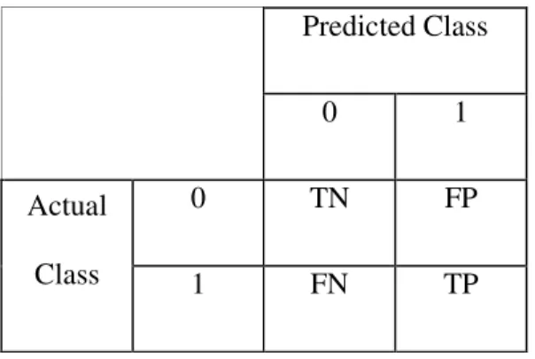
After a classifier is built, the performance of the model has to be tested whether the model really works or not. For this purpose, a set of rates are calculated by using the testing data that were never used during the training procedure. The results of the testing stage is reported using a simple statistical method which provides a window for the true positive rate, true negative rate, false-negative rate, false-positive rate and the success rate for the classifier under a given level of confidence.
To calculate the rates mentioned above, the confusion matrix has to be calculated at first. The structure of the confusion matrix is shown in Table3.1. The variables TP, TN, FP and FN that are used to demonstrate the confusion matrix show the number of instances that are classified as true positive, true negative, false positive and false negative. (Witten and Frank, 1999)
Table 3-1 The structure of the confusion matrix Predicted Class
0 1
0 TN FP
Actual
Class 1 FN TP
A true positive instance is a positive instance that is classified as positive. A false positive instance is an actually zero instance that is classified as positive. A true negative instance is a zero instance that is classified as zero. A false zero instances are a zero instance that is
classified as positive. In our case, the positive instances are forecasting tags that performs over IMKB and the zero instances are forecasting tags that perform below IMKB.
The false positive rate is the ratio that shows the proportion of the number of false positive instances to the total number of zero instances. The definition of the false positive rate is shown in Equation (3.23).
In our research predicting case 1 has more significance then case 0. Performance classifiers are measured by parameters called recall and prediction. The definition of recall is shown is equation (3.23) FN TP TP recall + = (3.233)
Precision shows us the prediction ratio of TP compared to all predictions for case 1. It gives the success ratio for our financial decisions for investment. The definition of precision is equation (3.24) FP TP TP precision + = (3.244)
The success rate is the ratio that shows the proportion of the number of correctly classified instances to the total number of instances. The definition of the success rate is shown in Equation (3.25).
FN FP TN TP TN TP sr + + + + = (3.255)
After calculating the point estimates of these rates, we can also report the Confidence Interval (CI) for each rate at 90 per cent and 95 per cent confidence levels. The upper and the lower limit of the confidence interval for each rate are calculated by using Equation (3.26). (Witten and Frank, 1999)
N in Equation (3.26) equal to the denominator part of the equation for each rate, and f is the point estimate for each rate. Z is the random variable that has a standard normal distribution (µ=0, σ=1). The value of z determines the confidence level. In order to calculate a CI for 90 per cent confidence level, z has to be set to 1.65. In order to calculate a CI for 95 per cent confidence level, z has to be set to 1.96.
N z N z N f N f N z f fuplow 2 2 2 2 2 , 1 4 2 + + − ± + = (3.266)
4. APPLIED METHODOLOGY AND RESULTS
4.1. Methodology
The balance sheet ratios that were considered in this work consist of 75 ratios and 225 synthetic ratios created by these ratios that are considered to be among the indicators of firms’ financial situation that affect the price of stock. These 75 ratios obtained from balance sheet of firms’ by calculated as described on Appendix A. It is explained in second chapter of this thesis how the ratios are used to form these synthetic ratios are calculated.
After the data table created, several statistical methods are applied to analyze the data. Application of analysis divided into 3 steps.
4.1.1. Step 1
225 synthetic ratios and the tag0, that created as described on chapter 2, enters to the first step on analysis. Student’s t-test is applied to data in order to determine which of the 225 synthetic ratios will be allowed for Linear Discriminant Analysis. In order to be on the safe side, we assumed unequal variances in the two classes. Student t-test result for step 1 could be seen at Appendix B where E.V is Equal Variance.
After this step least significant valued variables, that has smaller significant than p = 0.003, had been chosen for analysis. These variables are BV07, BV53, CV54, AV64, AV21, CV40, AV40, BV54, AV63 and BV08.
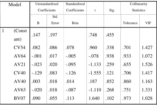
Before the Linear Discriminant Analysis, we have to prevent the collinearity between the selected variables. Linear Regression is run to measure Collinearity Statistics. Variance inflation factors (VIF) represent the collinearity between dependent variable and selected variables. Regression repeated after variables that has VIF value greater then 2, excluded from the analysis one by one. Then we reached the following table that contain the variables that pass the student t-test and has no collinearity.
Table 4-1 Collinearity Statistics for Step 1 Unstandardized Coefficients Standardized Coefficients t Sig. Collinearity Statistics Model B Std.
Error Beta Tolerance VIF
1 (Const ant) .147 .197 .748 .455 CV54 .082 .086 .078 .960 .338 .701 1.427 AV64 -.001 .017 -.005 -.078 .938 .933 1.072 AV21 -.023 .020 -.095 -1.133 .259 .655 1.526 CV40 -.129 .083 -.126 -1.555 .121 .706 1.417 AV40 .003 .018 .014 .187 .852 .860 1.163 AV63 -.020 .018 -.087 -1.110 .268 .751 1.331 BV07 .090 .055 .113 1.640 .102 .973 1.028 Dependent Variable: BV08
These variables enter for classifier. The Linear Discriminant Analysis (LDA) algorithm of Fisher (1936) is used. Discriminant analysis on SPSS used to classify these variables to obtain tag. LDA assigns a set of optimal weights to the variables in such a way that all different tag value are given a scalar index value that is below a certain threshold value. The index consists of the linear combination of the ratios weighted with the optimal weights. We use the within groups as covariance matrix.
The classification Function Coefficients are calculated as follows; Table 4-2 Classification Function Coefficients for Step 1
-,032 ,883 ,560 ,364 ,382 ,605 ,422 ,579 -,283 ,286 -3,385 -5,255 CV54 AV64 AV40 AV63 BV07 (Constant) ,000 1,000 tag0
From this table weights of variables could calculated as (tag0.1-tag0.0)
Then the equation obtained from step 1 is;
CV54 * 0.916 + AV64 * -0.196 + AV40 * 0.223 + AV63 * 0.157 + BV07 * 0.568 – 1.870
Classification result obtained from LDA analyses are;
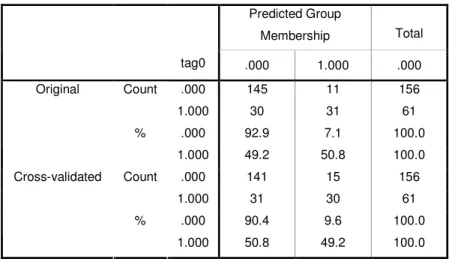
Table 4-3 Confusion Matrix for Step 1
Predicted Group Membership Total tag0 .000 1.000 .000 .000 145 11 156 Count 1.000 30 31 61 .000 92.9 7.1 100.0 Original % 1.000 49.2 50.8 100.0 .000 141 15 156 Count 1.000 31 30 61 .000 90.4 9.6 100.0 Cross-validated % 1.000 50.8 49.2 100.0
The first step is designed to give us a pattern (or an equation) that appears for stocks that outperform the ISE 100.
From these results we could measure the accuracy of analysis by calculating recall, precision and success ratio.
Recall value is;
492 . 0 30 31 30 = + = recall
Precision; 666 . 0 15 30 30 = + = precision Success ratio; 788 . 0 31 15 141 30 141 30 = + + + + = sr
Cross validation is done only for cross validated cases in the analysis. In cross validation, each case is classified by the functions derived from all cases other than that case.
After this step we reach some variables that affect our predictions. These ratios are;
V07: Non Paid-Up Share Probability (%)
If a company does not increase non paid-up shares and decrease the non paid –up share probability, equity capital has to be analyzed carefully. If the capital is not increasing too, it means there is a big problem about the stock. High non paid-up share probability signs equity capital increasing.
V40: Earning Per Share
By this ratio, it can be understood that whether if the owners or the shareholders are earning enough or not in Exchange of their investments. This ratio is very important for the people who think to invest to the related company. It is possible to find the profitability of
the share with dividing EPS by stock market value by using this value. This result is also one of the important guides for the investors.
V54: Current Year Income / Total Assets (%)
The rate of current year income in the total assets signs to the company’s profitability. After the company decided how the Income will be used, the paid-up shares are delivered and the rest is transferred to the shareholders equity, so the rate extent affects the transfer amount.
V63: Capital Sufficiency Ratio (%)
Capital Sufficiency Ratio is a numeric ratio that shows how many risk units is compensated by one unit capital. This sufficiency is determined at the international platform. It has to be at a minimum level about 8%.
V64: Inventories Turnover
If inventories turnover is high, it shows that the stocks are optimum and the companies have possibility to get more profit with less working capital; if turnover rate is low, that might sign to some problems at the selling activities.
4.1.2. Step 2
To increase selection sensitivity, methodology is applied to the data objected that pass the first step. For all data set, sum value is calculated by using the equation obtained from step 1. Data objects over cut off value (0) selected for second step. Similar calculations applied to the 42 data objects that passed from first step by using tag5 as tag value. The second
step is designed to give us a pattern (or an equation) that appears for stocks that outperform the ISE 100 by 5% provided that the stock has passed the step 1 test.
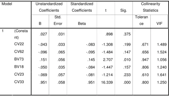
Student’s t-test is also applied to data in order to determine which of the 225 synthetic ratios will be allowed for Linear Discriminant Analysis on second step. In order to be on the safe side, we assumed unequal variances in the two classes. Student t-test result for step 2 could be seen from Appendix C
After this step least significant valued variables, that has smaller significant than p = 0.05, had been chosen for analysis. These variables are BV73, CV10, CV22, CV62, BV22, BV10, BV18, BV62, CV23, CV33 and CV35.
Collinearity analysis also repeated for step 2 with these variables. The variables that pass the student t-test and have no collinearity for step 2 are;
Table 4-4 Collinearity Statistics for Step 2
Unstandardized Coefficients Standardized Coefficients t Sig. Collinearity Statistics Model B Std. Error Beta Toleran ce VIF (Consta nt) .027 .031 .898 .375 CV22 -.043 .033 -.083 -1.308 .199 .671 1.489 CV62 -.096 .065 -.095 -1.484 .147 .656 1.524 BV73 .151 .056 .145 2.707 .010 .947 1.056 BV18 -.050 .035 -.084 -1.447 .157 .806 1.240 CV23 -.069 .057 -.081 -1.214 .233 .610 1.641 CV33 .951 .058 .951 16.339 .000 .800 1.250 1 Dependent Variable: CV35
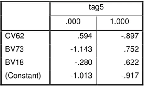
The classification Function Coefficients for step 2 are calculated as follows;
Table 4-5 Classification Function Coefficients for Step 2
tag5 .000 1.000 CV62 .594 -.897 BV73 -1.143 .752 BV18 -.280 .622 (Constant) -1.013 -.917
From this table weights of variables could calculated as (tag0.1-tag0.0)
Then the equation obtained from step 2 is;
CV62 * -1.491 + BV73 * 1.895 + BV18 * 0.902 + 0.096
Classification result obtained from LDA analyses are;
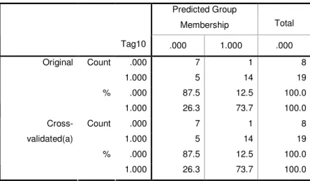
Table 4-6 Confusion Matrix for Step 2
Predicted Group Membership Total tag5 .000 1.000 .000 .000 13 6 19 Count 1.000 2 21 23 .000 68.4 31.6 100.0 Original % 1.000 8.7 91.3 100.0 .000 13 6 19 Count 1.000 3 20 23 .000 68.4 31.6 100.0 Cross-validated % 1.000 13.0 87.0 100.0
From these results we could measure the accuracy of analysis by calculating recall, precision and success ratio.
Recall value is;
87 . 0 3 20 20 = + = recall Precision; 769 . 0 6 20 20 = + = precision (3.27) Success ratio; 785 . 0 3 6 13 20 13 20 = + + + + = sr (3.28)
If we compare the results with first step we could see that we increase recall value while keeping precision and success ratio stable.
Financial ratios obtained from second step are;
V18: Market Capitalization
Market capitalization represents the public consensus on the value of a company. A corporation may be bought and sold through purchases and sales of stock, which will determine the price of the company's shares. Its market capitalization is this share price multiplied by the number of shares in issue, providing a total value for the company's shares and thus for the company as a whole.
V62: Cost of Sales / Net Sales (%)
The rate of sales cost in the net cost presents the sales process efficiency. It is aspired that the rate is reducing because this rate has a relation with company profitability, net sales profit margin.
V73: Equity Turnover
Equity turnover is used to calculate the rate of return on common equity, and is a measure of how well a firm uses its stockholders' equity to generate revenue. The higher the ratio is, the more efficiently a firm is using its capital. This ratio is also known as capital turnover.
4.1.3. Step 3
We could go further to increase selection sensitivity and finding more financial ratios that affect stock price. Our methodology is applied to the data objected that pass the second step. For all data set on step 2, sum value is calculated by using the equation obtained from
step 2. Data objects over cut off value (0) selected for third step. Similar calculations applied to the 27 data objects that passed from second step by using tag10 as tag value.
The third step is designed to give us a pattern (or an equation) that appears for stocks that outperform the ISE 100 by 10% provided that the stock has passed the step 1 and 2 tests.
Student t-test result for step 3 could be seen from Appendix 4.
After this step least significant valued variables, that has smaller significant than p = 0.01, had been chosen for analysis. These variables are AV09, AV03, AV73, AV08, AV66, CV56, AV42, AV63 and BV03.
Collinearity analysis also repeated for step 3 with these variables. The variables that pass the student t-test and have no collinearity for step 3 are;
Table 4-7 Collinearity Statistics for Step 3
Unstandardized Coefficients Standardiz ed Coefficients t Sig. Collinearity Statistics Model B Std. Error Beta Toleran ce VIF (Consta nt) .695 .820 .848 .405 AV03 -.075 .104 -.101 -.723 .477 .744 1.344 AV66 .082 .055 .217 1.473 .155 .672 1.489 CV56 1.125 .258 .616 4.362 .000 .734 1.362 1 AV63 -.042 .054 -.109 -.788 .439 .767 1.304 Dependent Variable: BV03
These variables enter for The Linear Discriminant Analysis classifier.
Table 4-8 Classification Function Coefficients for Step 3 tag10 .000 1.000 AV03 4.534 3.676 CV56 -.722 1.154 (Constant) -19.113 -12.397
From this table weights of variables could calculated as (tag0.1-tag0.0)
Then the equation obtained from step 3 is;
AV03 * -0.858 + CV56 * 1.876 + 6.716
Classification result obtained from LDA analyses are;
Table 4-9 Confusion Matrix for Step 3
Predicted Group Membership Total Tag10 .000 1.000 .000 .000 7 1 8 Count 1.000 5 14 19 .000 87.5 12.5 100.0 Original % 1.000 26.3 73.7 100.0 .000 7 1 8 Count 1.000 5 14 19 .000 87.5 12.5 100.0 Cross-validated(a) % 1.000 26.3 73.7 100.0
From these results we could measure the accuracy of analysis by calculating recall, precision and success ratio.
Recall value is; 736 . 0 5 14 14 = + = recall Precision; 933 . 0 1 14 14 = + = precision (3.29) Success ratio; 777 . 0 1 5 7 14 7 14 = + + + + = sr (3.30)
If we compare the results with the following steps, we could see that precision value get a very high level. To reach this precision value we make a concession from recall and success ratio. Although precision value is the most important value to show our success, we could stop calculating stock value on step 2 to get a higher recall value and success ratio.
Financial ratios obtained from third step are;
V03: Return On Assets (%) (ROA)
Return on assets tells an investor how much profit a company generated for each $1 in assets. The ROA graph is also a way to the asset intensity of a business. ROA measures a company’s earnings in relation to all of the resources it had at its disposal (the shareholders’ capital plus short and long-term borrowed funds). Thus, it is the most stringent and excessive test of return to shareholders. If a company has no debt, it the return on assets and return on equity figures will be the same.
V56: Net Profit Margin (%)
This number is an indication of company efficiency at cost control. If the net profit margin is higher. that means the company is effective at converting revenue into actual profit. The net profit margin is a good way of comparing companies in the same industry. since such companies are generally subject to similar business conditions. However, the net profit margins are also a good way to compare companies in different industries in order to gauge which industries are relatively more profitable.
5. CONCLUSION
A data mining model is built to make predictions for stock prices about one year in advance based on financial ratios obtained from the end-of-year balance sheets.
Model is built using balance sheet ratios of selected stocks between 1997 and 2005. Fishers’ Linear discriminant analysis used to make validation of data. Leave one out method allows not to reserve data for training.
Our model is constructed by 3 steps and each step has different equations to do stock selection. We choose a stock for investment after it gives positive results from all 3 equations.
The first step is designed to give us a pattern (or an equation) that appears for stocks that outperform the ISE 100.
Positive values obtained from first step enters second step similarly.
The second step is designed to give us a pattern (or an equation) that appears for stocks that outperform the ISE 100 by 5% provided that the stock has passed the step 1 test. Positive values from both step enters the third step of analysis.
The third step is designed to give us a pattern (or an equation) that appears for stocks that outperform the ISE 100 by 10% provided that the stock has passed the step 1 and 2 tests. When new balance sheet data announced, the financial ratios easily calculated and these values entered to the build model step by step.
According to this thesis, when a firm’s end-of-year balance sheet’s data pass this 3-step model, those stocks are expected to outperform ISE 100 by at least 10%.
6. REFERENCES
Analysing Your Financial Ratios; Retrieved, 2007 from
http://www.va-interactive.com/inbusiness/editorial/finance/ibt/ratio_analysis.html. 2007
Axler, S.(1995). Linear Algebra Done Right. Springer-Verlag New York. New York Inc.
Balakrishnama, S. Ganapathiraju, A.(1998). Linear Discriminant Analysis – A Brief
Tutorial.http://lcv.stat.fsu.edu/research/geometrical_representations_of_faces/PAPE RS/lda_theory.pdf
Banks, J. Carson, J. S. Nelson, B. L.. Nicol. D. M. (2001) Discrete-Event System
Simulation. Third Edition. Prentice Hall. New Jersey.
Boduroğlu, I. (2007). A Pattern Recognition Model for Predicting a Financial Crisis in
Turkey: Turkish Economic Stability Index.
Costello, C. Kendall, B. (2003). Hypothesis Testing. http://www.bren.ucsb.edu/
Duchene, J. Leclercq, S. (1998). An Optimal Transformation for Discriminant and
Principal Component Analysis. IEEE Transactions on Pattern Analysis and Machine Intelligence. Vol. 10. No. 6. pp. 978-983. November.
Finnet. Data Provider. (www.finnet.com.tr)
Fisher, R. A. (1936). The Use of Multiple Measurements in Taxonomic Problems. Annals
of Eugenics. v. 7. pp. 179-188. Cambridge University Press.
Fukunaga, K. (1990). Introduction to Statistical Pattern Recognition. Academic Press. San Diego. California.
Han, J. Kamber, M. (2001). Data Mining: Concepts And Techniques. San Francisco. Ca: Morgan Kaufmann.
Kantardzic, M. (2003). Data Mining - Concepts. Models. Methods. and Algorithms. IEEE and Wiley Inter-Science.
Kent, J.T.. Bibby, J.M. (1979). Multivariate Analysis. Academic Press.
Joo, S. W. (2003). Linear Discriminant Functions and SVM. http://image.pirl.umd.edu/ KG_VISA/LDA_SVM/swjoo_LinearClassifiers.pdf
Lin, C. C. Chen, A. P. (2001). A Method for Two-Group Fuzzy Discriminant Analysis. International Journal of Fuzzy Systems. Vol. 3. No. 1. pp.341-345. March.
Martens, H.A. Dardenne, P. (1998). Validation and verification of regression in small data sets 44. 99-121.
Stone, M.(1977). An Asymptotic Equivalence of Choice of Model by Cross-Validation and Akaike’s Criterion J. R. Stat. Soc.. B. 38. 44-47.
Vanstone, B. Finnie, G. Tan, C. (2004). Evaluating the Application of Neural Networks and Fundamental Analysis in the Australian Stock market
Weisstein, E. W. (1999). Beta Function. Concise Encyclopedia of Mathematic. http://icl.pku.edu.cn/yujs/MathWorld/math/b/ b153.htm
Witten, I. H. Frank, E. (1999). Data Mining: Practical Machine Learning Tools and Techniques with Java Implementations. Morgan Kaufmann Publishers. San Francisco.
Zhang, D. Zhou, L. (2004) Discovering Golden Nuggets: Data Mining In Financial
Application. Ieee Transactions On Systems. Man. And Cybernetics Discovering Golden Nuggets: Data Mining
7. APPENDIX
7.1. APPENDIX A ( Calculation of Ratios)
Table 7-1 Calculation of Ratios
Variable Financial Ratio Name Financial Ratio Calculation
V01 Asset Growth Rate (%)
([TOTAL ASSETS]-Previous Year's[TOTAL ASSETS])/Absolute Value(Previous Year's[TOTAL ASSETS])*100 V02 Asset Turnover [NET SALES]/[TOTAL ASSETS] V03 Return On Assets (%)
[CURRENT YEAR'S PROFIT OR LOSS]/[TOTAL
ASSETS]*100
V04
Total Assets / Marketable Securities [TOTAL ASSETS]/[MARKETABLE SECURITIES] V05 Receivables Turnover [NET SALES]/[Short-Term Receivables] V06 Collection Ratio 365/([NET SALES]/[Short-Term Receivables]) V07
Non Paid-Up Share Probability (%)
([Revaluation Of Tangible Fixed Assets]+[Issue Premium]+[Extraordinary Reserves])/[Capital Stock]*100 V08 Debt/Equity Ratio (%) ([SHORT-TERM LIABILITIES]+[LONG-TERM LIABILITIES])/[EQUITY]*100 V09
Beneficiation Coefficient from Debts (Times)
1/((([EQUAL
STOCK]-[Revaluation Of Tangible Fixed Assets])/([TOTAL ASSETS]-[Revaluation Of Tangible Fixed
Assets]))*([OPERATING
PROFIT or LOSS]/([PROFIT OR LOSS FOR THE
PERIOD]+[FINANCIAL EXPENSES (-)])))
V10 Gross Profit Margin (%)
[GROSS SALES PROFIT or LOSS]/[NET SALES]*100
V11 Current Ratio
[CURRENT ASSETS]/[SHORT-TERM LIABILITIES]
V12
Net Profit or Expenses From Other Operations
([INCOME FROM OTHER OPERATIONS]-[LOSS and EXPENSES FROM OTHER OPERATIONS (-)])/[NET SALES]
V13
Profit Margin from Other Operations (%)
[INCOME FROM OTHER OPERATIONS]/[NET SALES]*100
V14 Long Term Assets Turnover
[NET SALES]/[LONG-TERM ASSETS]
V15
Long Term Assets / Total Assets (%)
[LONG-TERM ASSETS]/[TOTAL ASSETS]*100
V16 P/E Ratio
End-of -Period Market Capitalization/(Last Yearly Balance Sheet[CURRENT YEAR INCOME or LOSS]-Previous Year’s[CURRENT YEAR
INCOME or LOSS]+[CURRENT YEAR INCOME or LOSS]
V17
Market Capitalization / Book Value
Market Capitalization / Book Value
V18 Market Capitalization Market Capitalization V19 Current Assets Turnover [NET SALES]/[CURRENT
ASSETS]
V20 Current Assets / Total Assets (%)
[CURRENT ASSETS]/[TOTAL ASSETS]*100
V21 Deficiency Coverage Ratio
(([SHORT TERM LIABILITIES]+[LONG TERM LIABILITIES])-([Liquid Assets]+[Marketable Securities]+[Short-Term Receivables]+[Other short-Term Receivables]))/[Inventories]
V22 Operating Profit Growth Rate (%)
([OPERATING PROFIT or LOSS]-Previous Year's[OPERATING PROFIT or LOSS])/Absolute Value(Previous Year's[OPERATING PROFIT or LOSS)*100
V23 Operating Profit Margin (%)
[OPERATING PROFIT or LOSS]/[NET SALES]*100
V24
Earnings Before Interest. Tax. Depreciation and Amortization (EBITDA)
(OPERATING PROFIT or LOSS]+[AMORTIZATION EXPENSES . DEPLETION ALLOWANCE ])/[NET SALES]
V25
Non-Operating Profit / Operating Profit (%)
[NON-OPERATING
PROFIT]/[OPERATING PROFIT or LOSS]*100
V26
Operating Expenses / Net Sales (%)
[OPERATING EXPENSES(-)]/[NET SALES]*100
V27 Operating Costs / Net Sales (%)
([SALES COST )]+[OPERATING EXPENSES (-)]+[NON OPERATING EXPENSES]+[FINANCIAL EXPENSES (-)])/[NET SALES]*100
V28 Interest Coverage
(([CURRENT YEAR INCOME or LOSS]+[FINANCIAL
EXPENSES (-)])/[FINANCIAL EXPENSES(-)])-1
V29 Financial Loans / Equity (%)
([Financial Debts]+[Financial Debts])/[EQUITY]*100
V30 Financial Loans / Total Liabilities
[Financial Debts]/([SHORT-TERM DEBTS]+[LONG-Debts]/([SHORT-TERM DEBTS])
V31
Financial Expenses + Profit Before Tax / Gross Sales
(([FINANCIAL EXPENSES (-)]+[CURRENT YEAR PROFIT or LOSS])/[NET SALES])*100
V32
Financial Expenses / Inventories (%)
([FINANCIAL EXPENSES (-)]/[Inventories])*100
V33 Financial Expenses / Total Costs
[FINANCIAL EXPENSES (-)]/([SALES COST)]+[OPERATING EXPENSES (-)]+[NON-OPERATING EXPENSES and LOSS]+[EXTRAORDINARY EXPENSES and LOSS]+[FINANCIAL EXPENSES (-)])*100 V34
Financial Expenses / Total Liabilities (%) [FINANSMAN GIDERLERI (-)]/([KISA VADELI BORCLAR]+[UZUN VADELI BORCLAR])*100 V35
Financial Expenses / Operating Costs (%) [FINANCIAL EXPENSES )]/([SALES COST )]+[FINANCIAL EXPENSES )]+[OPERATING EXPENSES (-)]+[NON-OPERATING
V36
Financial Expenses / Net Sales (%)
([FINANCIAL EXPENSES (-)]/[NET SALES])*100
V37
Financial Expense Growth Rate (%) (([FINANCIAL EXPENSES (-)]-Previous Year's[FINANCIAL EXPENSES(-)])/Absolute Value(Previous Year's[FINANCIAL EXPENSES(-)]))*100
V38 Market Capitalization/Cash Flow
Market Value / (FOUR
QUARTERS(CURRENT YEAR NET PROFIT or PROFIT)- (FOUR
QUARTERS(AMORTIZATION EXPENSES). DEPLETION ALLOWANCE))
V39 Liquid Assets / Current Assets (%)
[Liquid Assets]/[CURRENT ASSETS]*100
V40 Earning Per Share
[CURRENT YEAR NET PROFIT or LOSS]/([Share Quantity])
V41
Liquid Assets/Net Working Capital ([Liquid Assets]+[Marketable Securities]+[Short-Term Receivables]+[Other short-Term Receivables])/([CURRENT ASSETS]-[SHORT-TERM LIABILITIES)) V42 Leverage Ratio (%) ([SHORT-TERM LIABILITIES]+[LONG TERM LIABILITIES])/[TOTAL ASSETS)]*100 V43
Short-Term Fin. Loans / Total Liabilities (%)
[Financial Debts]/([SHORT TERM LIABILITIES]+[LONG TERM LIABILITIES])*100 V44 Short-Term Liability Growth (%) ([SHORT TERM
LIABILITIES]-Previous Year's [SHORT TERM LIABILITIES])/Absolute Value(Previous Year's[SHORT TERM LIABILITIES])*100
V45
Short-Term Liabilities / Net Sales (%)
([SHORT TERM LIABILITIES]/[NET SALES])*100
V46
Short-Term Liabilities / Total Liabilities (%) [SHORT TERM LIABILITIES]/([SHORT TERM LIABILITIES]+[LONG TERM LIABILITIES])*100 V47 Acid-Test Ratio ([Liquid Assets]+[Marketable Securities]+[Short Term
Receivables]+[Other Short Term Receivables])/[SHORT TERM LIABILITIES]
V48 Tangible Fixed Assets Turnover
[NET SALES]/Average[Tangible Fixed Assets]
V49
Tangible Fixed Assets/(Shareholders
Equity+Long Term Liabilities)
[Tangible Fixed
Assets]/([EQUITY]+[LONG TERM LIABILITIES])
V50
Marketable Securities Growth Rate (%) ([Marketable Securities]-revious Year's[Marketable Securities])/Absolute Value(Previous Year's[Marketable Securities])*100 V51
Marketable Securities / Total Assets (%) ([Marketable Securities]/[TOTAL ASSETS])*100 V52 Cash Ratio ([Liquid Assets]+[Marketable Securities])/[SHORT TERM LIABILITIES] V53
Current Year Income /