A N ANALYSIS OF OIL DEMAND I N TURKEY
ZEYNEP DENİZ
103626002
ISTANBUL BILGI UNIVERSITY
INSTITUTE OF SOCIAL SCIENCES
MSc. in Financial Economics
Supervised by:
SİNA ERDAL
A N ANALYSIS OF OIL DEMAND I N TURKEY
TÜRKİYE İÇİN PETROL TALEBİ ANALİZİ
ZEYNEP DENİZ
103626002
Sina Erdal
Ege Yazgan
Koray Akay
Tezin Onaylandığı Tarih : 06.02.2006
Toplam Sayfa Sayısı: 30
Anahtar Kelimeler
1) Fiyat ve gelir elastikiyetleri
elasticities
2) Vergilendirme
3) Dışsal etkiler
4) Petrol fiyatları
5) Bütçe Açığı
Key Words
1) Price and income
2) Taxation
3) Externalities
4) Oil Prices
5) Budget Deficit
A B S T R A C T
Using quarterly data from 1992-2004, we conduct an econometric investigation of the short and long-run price and income elasticities of gasoline consumption in Turkey. We find that short-run income elasticity is 0.58, short-run price elasticity is -0.15 (statistically insignificant) and the long-run price elasticity is approximately -0.38, long-run income elasticity is approximately -0.23 (statistically insignificant). Our findings suggest that the recent heavy taxation of oil derivatives in general and gasoline in particular may be optimal in Turkey.
ÖZET
Bu tezde 1992-2004 yılları için üç aylık veriler kullanılarak kısa ve uzun dönem için benzin tüketiminin fiyat ve gelir elastikiyetleri ekonometrik bir araştırma sonucunda ortaya konmuştur. Kısa dönem gelir elastikiyeti 0.58, kısa dönem fiyat elastikiyeti -0.15 (istatiksel olarak anlamsız) ve uzun dönem fiyat elastikiyeti -0.38, gelir elastikiyeti ise -0.23 (istatiksel olarak anlamsız) olarak tahmin edilmiştir. Bulgularımıza göre devletin petrol ürünleri üzerine koyduğu vergi optimal olabilir.
A C K N O W L E D G E M E N T S
I gratefully acknowledge my advisor Sina Erdal who has given me invaluable comments throughout this dissertation. Without his consideration, support and guidance, it would be difficult to complete this study.
I would like to thank in particular, to my professors in the Financial- Economics Department for their worthy suggestions.
Finally, I am grateful to my family and friends for their continuing support, understanding and encouragement in the preparation process of my thesis.
T A B L E O F C O N T E N T S Abstract i Acknowledgements i i List of Tables iv List of Figures iv 1. INTRODUCTION 1 1.1. Literature Review 2
2. OPTIMAL TAX LEVEL AND EFFECTS OF TAXATION POLICY 4
3. COMPARISON OF THE TAX COMPONENT: TURKEY VS. EU
COUNTRIES 7
4. TAXATION SYSTEM OF OIL CONSUMPTION I N TURKEY 10
5. ECONOMETRIC ANALYSIS OF OIL DEMAND I N TURKEY:
ESTIMATING ELASTICITIES 11
5.1. Data Description 11 5.2. Diagnostic Tests Performed on The Data 12
5.2.1. Test for Endogeneity 13 5.2.2. Omitting the Irrelevant Variables and Testing for Endogeneity
17
5.2.3. Seasonal Adjustment 19
5.3. Specifying Final Estimation 20 5.4. Residual Test Result of the Final Specification 20
5.5. Estimating Short-run and Long-run Elasticities 21
REFERENCES 26 APPENDIX 28
L I S T O F T A B L E S
Table 1: EU Countries Gasoline Price Structure, January 2005 8 Table 2: Super Gasoline Price Structure, 13 January 2005 9
Table 3: Endogeneity test, initial specification 13
Table 4: Correlations between IVs and Pt 14
Table 5: Correlations between IVs and error terms 14 Table 6: Endogeneity test, first specification 15 Table 7: Endogeneity test, second specification 16 Table 8: Endogeneity test, initial specification 17 Table 9: Endogeneity test, first specification 18 Table 10: Endogeneity test, second specification 18
Table 11: Final Specification 20 Table 12: Lag-coefficients of Long-run Price elasticity 22
Table 13: Lag-coefficients of Long-run Income elasticity 23
L I S T O F F I G U R E S
Figure 1: Super Gasoline Price Structure 9 Figure 2: Comparison of the World Oil Price and Price at the Pump in
Turkey 10 Figure 3: Seasonal Adjustment for Quantity Series 19
1. I N T R O D U C T I O N
Oil is an ever-larger economic input for Turkey, a country with a large population and rapidly increasing industrial output. In this study, we examine the price and income elasticities for the most significant oil derivative, namely, gasoline, in Turkey due to its significant share in oil consumption. We deem this an important research topic for various reasons. First o f all, since Turkey has negligible oil production of its own, its oil import bill contributes significantly to its current account deficit. The country's current account deficit, one of the highest in the developing world as a percentage of GDP, in turn, is one major factor behind its recent economic crises which have had severe consequences for the country's GDP growth. Secondly, like almost all other world governments, the Turkish government too uses taxation at the pump to regulate the prices o f oil derivatives. While taxation at the pump is economically desirable due to the negative externalities such as pollution and traffic congestion that the use o f petroleum derivatives produces, in the Turkish case, the curbing o f such externalities seems to have taken a backseat to raising revenue for the government. Indeed, in 2004, taxes collected from petroleum products made up nearly 20% of all budget revenues. This conjecture is further supported by the fact that, relative to per capita income, these taxes in Turkey were one o f the highest in the world as of the end of 2005. Such high levels have been attained as a result of continuous increases in taxes as a part of the IMF program that Turkey has agreed to follow after the economic crisis in 2001. The period o f high economic and political uncertainty and chaos followed by a rapid agreement with the IMF following the 2001 economic crisis raises the possibility that the Turkish government's IMF mandated policy of extremely high taxation o f energy products in general and oil derivatives in particular may be a knee-jerk reaction. We also conjecture that this primary goal o f raising budget revenues is followed closely in importance by the desire to curb the current account deficit, as mentioned above.
The main objective o f this study is to determine the oil demand function for Turkey by specifying an econometric model. With the help o f this econometric
model, short-run and long-run income and price elasticities o f gasoline consumption o f oil demand are estimated. The final step is deciding whether imposing "large" tax levels on oil derivative products is optimal or not by evaluating these elasticity numbers in comparison with the other developing countries.
The thesis is organized as follows; in section 1 we introduce our thesis and approach and do a literature review. In section 2, the specification of the optimal tax level is discussed and then the potential effects of taxation on the economy are introduced. In the 3r d section, tax component o f oil price in different countries are given and it is demonstrated that Turkey takes the first place between EU countries. In section 4, we briefly summarize the taxation system o f oil products in Turkey. The next part, section 5, explains the econometric procedure and data to construct the consumption model o f oil to estimate the elasticities, and the last part, section 6, is the conclusion of this thesis.
1.1. Literature Review
There are only a few recent research papers about the dynamics o f oil demand in Turkey. A. Kibritcioglu (1999) constructs a V A R model by using monthly data for oil consumption and prices for the years between 1986 - 1998. He reaches the conclusion that imported crude oil prices have a small affect on inflation in Turkey. Another paper by Mesutoglu (2001) estimates the price elasticity o f gasoline consumption for the years between 1990 - 1999 as -41 %. The explanatory variables used are population, prices o f oil derivatives, prices o f substitute goods, number o f tourists visiting Turkey and seasonal dummy variables. A more current paper by Kirmanoglu et. al. (2003) uses monthly data between 1993 and 2003 to estimate income and price elasticities of oil demand. Their main concern, however, is air pollution that is caused by fuel consumption. Their findings indicate that the elasticities are very close to unit elasticity. Therefore, they conclude that increasing fuel taxes for more polluting
fuels can be an effective policy against curbing air pollution as well as raising revenues for the government.
As for studies o f oil demand in general, Kennedy (1974) models oil markets separately for the United States, Canada, Latin America, Europe, the Middle East, Africa and Asia. In his model the exogenous variables include the regional supply and demand equations, the technology of refining and government policy variables. Similar to our thesis, his paper describes the structure o f an econometric model o f the world oil market and presents results that are used in forecasting and policy simulations. The results o f simulations from the model suggest that an export duty of half of the current level, about $ 3.5 is most likely to occur in the long run. Kennedy also finds that the world oil price hikes which occurred in late 1973s are not likely to persist in the future. Ramsey, et. al, (1975) uses simultaneous equations model to estimate the price elasticity o f gasoline demand in the USA. The price elasticity in this paper is equal to -0.74. Baltagi et. al (1983) study the gasoline demand in OECD countries. Wasserfallen et. al (1988) study the relationship between gasoline consumption and vehicle stock in Switzerland. Dahl et. al (1991) in their paper concerning gasoline demand have found that income and price are the most important variables defining gasoline demand. For a developing country, the paper o f Garbacz (1989) can be a good reference in which gasoline demand in Taiwan is examined and price elasticity is found as -0.81. Ibrahim et. al (1990) attempt to identify the factors that have determined the level and pattern o f energy demand in developing countries during the 1970s and early 1980s. Differently from most of the other elasticity estimates, Goel (1994) uses the quasi-experimental method which is appropriate for the commodities that have fairly stable prices and whose prices change as a result of tax changes for calculating the price elasticity. Gasoline taxation elasticity is found as 0.075 for the USA for the years 1952
-1986 in this paper. In the research by McRae (1994), gasoline demand is specified for developing countries. In this study, the price elasticities for the middle income countries range from -0.30 to -0.32 in the short-run and -0.58 in the long-run. The income elasticities for the middle-income countries range from
0.57 to 0.67 in the short-run and 1.70 in the long-run. The price elasticities for the low-income countries range from -0.12 to -0.17 in the short-run and -0.31 in the long-run. The income elasticities for the low-income countries range from 0.74 to 0.79 in the short-run and 1.18 in the long-run. Another recent research is done by Alves et. al (2003). In their paper, by using cointegration techniques, they estimate the price elasticity o f gasoline, cross-price elasticity between gasoline and alcohol and the income elasticity o f gasoline. Price elasticity o f gasoline is found to be inelastic in the long-run and completely inelastic in the short run revealing important implications for policymakers.
2. O P T I M A L T A X L E V E L AND E F F E C T S O F T A X A T I O N P O L I C Y
World energy consumption is increasing along with the population and global industrialization. Oil, with its large share in the total world energy consumption, has been a very important commodity for social and economic development o f countries. Differently from the other energy types, oil is both an input for nearly all o f the industries and a necessity good with no close substitutes that is consumed by the public. Due to its economic importance, decisions regarding taxation o f oil products must be made with significant care. While taxation brings revenues for a government, it may have adverse effects to the economy.
As the policy maker authority, one o f the important subjects that a government must handle regarding the supply and demand for oil is managing the externalities that are caused by oil consumption. The most significant externality is air pollution. Another one is traffic congestion, especially in urban areas. Since currently almost all vehicles on the road need some petroleum derivative to run, one way o f making vehicle usage costlier is by taxing oil derivative products to curb the resulting externalities. The most popular tool used by governments around the world for this purpose is taxation at the pump. Even though taxation is the tool o f choice for governments for limiting externalities and increasing budget revenues, since taxes in general lead to distortions in the economy, determining the optimal level o f taxation becomes a key issue. This
necessitates a good understanding o f the income and price elasticities o f oil demand and characteristics o f a country. The optimal taxation theory suggests a hump-shaped progression o f marginal taxation rate. The maximum tax receipts occur at the maximum point of this hump-shaped curve which gives the optimal tax level for the relevant industry. In Turkey's case, we conjecture that the tax level is on the right side o f this maximum point which means the tax rate is higher than optimal, hence the tax receipts are below the maximum amount.
I f the government sets taxes suboptimally, there will be two major adverse effects on an economy. The first one o f these adverse affects is factor substitution. A basic production function consists o f three different inputs, namely, labor (L), capital (K) and energy (E). When the price of oil gets higher, so does the cost of energy. This leads to a shift from energy to labor and capital. I f the increase in the price o f a factor is caused by taxation, the input mix will be distorted and there will be efficiency loss in the economy. Hence, the inefficient use of oil decreases the competitive power of an economy.
Given a fixed capital stock and limited ability to substitute away from the higher priced factor, the production effects of a pure cost increase are closely related to the share of energy in the economy. This is the GNP share of energy multiplied by the percent price change which gives a first-order approximation to the contraction in production capacity. In the short run, this change marks the maximum impact on the economy. As a result, both combinations o f inputs would produce less output than the efficient combination that existed prior to the price change. Thus, the capacity of the economy will have decreased.
Secondly, as a result o f the high oil prices, the demand o f legal oil products decreases and demand for illegal oil products gets a higher share in total oil consumption. As a result of the shift in demand, the government may not be able to collect projected tax revenues. Illegal oil consumption has another indirect effect in the economies. It is known that the illegally produced oil derivative products are not qualified as the legal ones as a result o f their refining and
storage processes. These lower-quality oil derivative products may damage the vehicles or decrease their economic life. The consumers' choice to use the low quality fuel is another form of input substitution away from energy to capital. Today, in Turkey, there is indeed a market for the illegally produced oil. According to the Chamber of Commerce (Ankara Ticaret Odası, ATO), the tax loss due to smuggled oil in Turkey is nearly 2.5 billion dollars per year. ATO claims that for the years between 1996 - 2003, the increase in the number of cars is nearly 40%, however the increase in the oil consumption is only 11% and the difference between these rates is likely met by smuggled oil. As a result of this illegal importation and consumption, the production and consumption of oil may be underestimated. This underestimation may contribute to making taxation decisions of policymakers suboptimal.
An indirect adverse effect of high oil price as a result of the large tax component is economic recession. Economic theory offers several explanations of how oil price increases could trigger a recession. Oil is, for practical purposes, inevitably used and difficult to substitute for generally in the short run. A standard macroeconomic analysis suggests that consumers, faced with a price run-up, would attempt to maintain oil consumption in the short run by reducing the purchases of other goods and services. The oil price increase would tend to be inflationary and that increase in the general price level would reduce the real money balances held by the public which is the stock of money adjusted for changes in its value caused by price-level changes. Consequently, the public would reduce their spending on goods and services below what would be required to keep their oil consumption constant to restore their real balances. This decrease in aggregate demand would trigger a recession in the economy. The government, through monetary policy actions, could increase the money supply to accommodate the public's reaction to real balances. The monetary authority's policy would depend on their evaluation of the impact of the price shock on subsequent levels of economic activity and on their concern with
inflationary pressures. An empirical study that is studied by Meyermans1, 2005, estimates that a permanent 25 percent oil price increase, in the long run, reduces aggregate private sector output by 0.27 percent in the euro area, 0.30 percent in the Western non-euro EU Member States, 0.33 percent in the United States, and 0.23 percent in Japan. Price increases also affect the supply side of the economy by influencing the costs of producing the same volume of GDP that was produced prior to the shock and by changing the amount o f other factors o f production such as labor, capital, and other materials relative to oil.
3. COMPARISON O F T H E T A X COMPONENT: T U R K E Y VS. E U C O U N T R I E S
In most world economies, taxes are the largest component o f the price o f oil products. This is also true for Turkey, but the proportion o f taxes in the total price in Turkey is among the highest in the world. We should note that this is a relatively recent phenomenon. At the beginning of 1990 the pump price of super gasoline in Turkey was nearly 53 cents, while at the beginning of the 2005 it was $1.60. However, the world price of oil in the same period increased only roughly 100%. The gap between the world price and price in Turkey comes from the costs such as transportation cost, retailer margin and tax component imposed by Turkish government. The costs and retailer margins have behaved in predictable ways in this period while proportional taxes have increased substantially. At the beginning o f 1990 the tax component was 56% o f the total price, but at the beginning of 2005, it became nearly 73% o f the total price. According to the research by the International Energy Agency (IEA) in 2000, Turkey ranked only
12t h among 26 OECD countries2 with a 61.2% tax component. We must also note that the tax component o f the pump price in Turkey has a significantly higher rank among those countries when it is measured relative to per capita income. The first country in 2000 was U K with 75.6%. However, according to
1 Meyermans and Brusselen, "The Macroeconomic Effects of an Oil Price Shock on the World
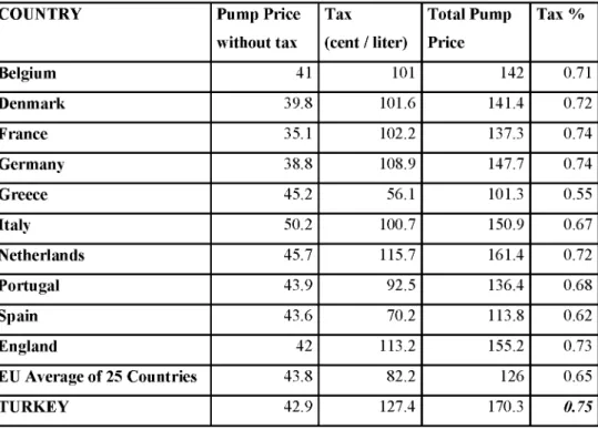
research done by Tupras. A.S., as of January 2005 Turkey jumped to the number one spot in the ranking between EU countries with a 75% tax component. This result is illustrated in the following table.
Table 1: E U Countries Gasoline Price Structure, January 2005
C O U N T R Y Pump Price Tax Total Pump Tax %
without tax (cent / liter) Price
Belgium 41 101 142 0.71 Denmark 39.8 101.6 141.4 0.72 France 35.1 102.2 137.3 0.74 Germany 38.8 108.9 147.7 0.74 Greece 45.2 56.1 101.3 0.55 Italy 50.2 100.7 150.9 0.67 Netherlands 45.7 115.7 161.4 0.72 Portugal 43.9 92.5 136.4 0.68 Spain 43.6 70.2 113.8 0.62 England 42 113.2 155.2 0.73 E U Average of 25 Countries 43.8 82.2 126 0.65 T U R K E Y 42.9 127.4 170.3 0.75
Source: Tupraç Report, January 2005
Furthermore, the tax component in Turkey is 10% higher than the average of the 25 EU countries.
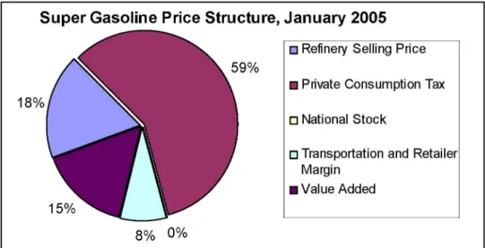
On January 2005, the refinery price of super gasoline was 0.42 Y T L / liter but the price at the pump was 2.33 Y T L / liter. The pump price composition of super gasoline is given in Table 2 and is illustrated in Figure 1.
Table 2: Super Gasoline Price Structure, 13 January 2005
Super Gasoline Price Structure 13.January.2005
Y T L / liter Refinery Selling Price 0.42 Private Consumption Tax 1.36
National Stock 0.0015
Transportation and Retailer Margin 0.19
Value Added Tax 0.36
Pump Price 2.33
Source: Tupras. Report, January 2005
Figure 1: Super Gasoline Price Structure
Super Gasoline Price Structure, January 2005
A
1 8 % /
\ 59%
)
• Refinery Selling Price • Private Consumption Tax • National Stock
15%
• Transportation and Retailer Margin
• Value Added
8% 0%
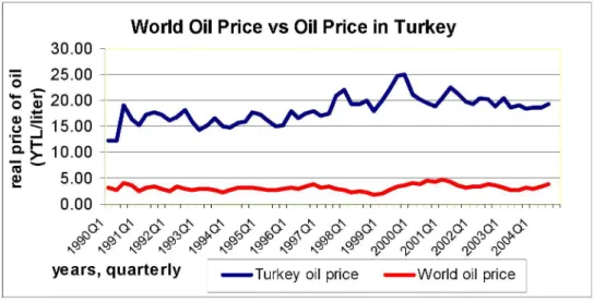
The increase in pump prices in Turkey is not parallel to the increase in world oil prices. This is demonstrated in Figure 2.
Figure 2: Comparison of the World Oil Price and Price at the Pump in Turkey
5
World Oil Price vs Oil Price in Turkey
30.00 n 25.00 20.00 15.00 y 10.00 5.00 0.00 oN Nd> d> d> .d> <d> d> , , Q > d> d> ^ Nd> „d> „p> J D > # K # K « ^ ^ K « ^ *\ *\ *\ \ K # ^ ^ «? «? <V 'V v 'V
years, quarterly Turkey oil price World oil price
We should also note that in Figure 2, world oil price has a smoother trend than the Turkey oil price. The difference is mainly due to the volatility of the tax component in the oil price in Turkey.
4. T A X A T I O N S Y S T E M O F O I L CONSUMPTION IN T U R K E Y
This section contains the basis of Turkish taxation system of oil products in Turkey. The Turkish oil market had been heavily regulated before significant liberalization that took place in 1989-1990. Until 1990 domestic oil producers had to sell their production to TUPRAS. Oil product prices were set by the government. Under Law No. 79 of 1989, importers, refineries and oil distribution and retailing companies were allowed to set prices freely for crude oil and petroleum products. However, the same law enabled the government to determine "fundamental principles of purchase, sale and distribution of crude oil and petroleum products". The outcome of this reform was that oil producers were allowed to sell 35% of their production freely. Oil product imports and exports were liberalized in 1989; all refineries and retailers with minimum storage capacities were granted import licenses. However, the government continued to prescribe annual oil import programs with the stated purpose of
matching refinery requirements in terms of quantity and quality. Tüpraş's ex-refinery prices for oil products remained subject to government approval.
Today, Turkey's main tax on oil products is the fuel consumption tax (FCT). To eliminate the effects of oil price fluctuations and the pronounced exchange rate fluctuations of the Turkish lira against the dollar on domestic oil prices, the government linked this tax to a mechanism called the Fuel Price Stabilization Fund (FPSF), as of 5 February 2000. The purpose of this fund is to stabilize domestic oil prices. The tax rate is inversely proportional to developments in international oil prices and the exchange rate of the Turkish lira against the dollar.
5. E C O N O M E T R I C A N A L Y S I S O F O I L DEMAND IN T U R K E Y : E S T I M A T I N G E L A S T I C I T I E S
5.1. Data Description
In order to investigate the empirical relationship among oil consumption in Turkey, oil prices and income levels, a log-log demand model is employed. We used quarterly data for the years between 1992 and 2004. We get 1990 as the base year for all series, however we could not use the data for years 1990-1992 since quantity data is not available for these years. The reason to use the double¬ log functional form instead of linear form is that the estimated coefficients on price and income series directly give the price and income elasticities of oil demand.
Oil consumption data consists of quantities of super, normal and unleaded gasoline consumed. For the years between 1992 and 2000 quarterly data for oil consumption in million tons is obtained from Petrol İşleri Genel Müdürlüğü (PIGM), the government oil directorate of Turkey. For the years between 2000 and 2004, the source for the quantity series is the oil market report of Turkey issued by the International Energy Agency Organization. The magnitudes of the
consumption data for those years are consistent with the yearly consumption data that is published by PIGM.
The price series is the quantity-weighted average real price of the three types of gasoline sold in Turkey. Inflation, current account deficit, budget deficit, and GDP data are obtained from the Central Bank of Turkey. Current account deficit and budget deficit data are converted to real terms and then weighted by real GDP. World oil price is obtained from the World Bank in dollars per barrel and it is converted to real Y T L per liter.
The data used in the analysis are quarterly time series from 1992:1 to 2004:4
lnq: Natural logarithm of the total of super, normal and unleaded gasoline consumption
lnp: Natural logarithm of the quantity-weighted average real price of super, normal and unleaded gasoline
lnpw: Natural logarithm of World oil price, converted into real Y T L per liter lngdp: Natural logarithm of Gross Domestic Product of Turkey
Bd: Real Budget deficit over GDP Ca: Real Current account over GDP
lntax: Natural logarithm of the tax component of the gasoline price in real terms
6.1.Diagnostic Tests Performed on The Data
In this section, some preliminary tests are performed before the final specification. These tests are necessary to evaluate the appropriateness of the chosen variables.
6.1.1. Test for Endogeneity
To determine whether price is endogenous in the demand equation, we use the Hausman test3. The steps of the Hausman test are as follows:
We initially estimate the equation:
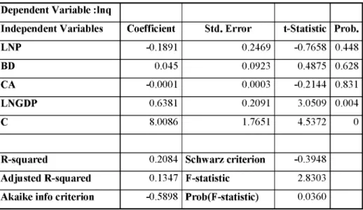
ln Qt = J30 + J31 ln Pt + J32 ln CAt + J33BDt + J34 ln GDPt + ut (1)
This is a static model that shows the short-run elasticities. J31 is the price elasticity of demand while J34 is its income elasticity. However, in the next sections, we will estimate a dynamic model with appropriate explanatory variables in order to determine both short-run and long-run elasticities. The estimation result of the initial demand equation is given in Table 3.
Table 3: Endogeneity test, initial specification
Dependent Variable :lnq
Independent Variables Coefficient Std. E r r o r t-Statistic Prob.
LNP -0.1891 0.2469 -0.7658 0.448
BD 0.045 0.0923 0.4875 0.628
C A -0.0001 0.0003 -0.2144 0.831
L N G D P 0.6381 0.2091 3.0509 0.004
C 8.0086 1.7651 4.5372 0
R-squared 0.2084 Schwarz criterion -0.3948
Adjusted R-squared 0.1347 F-statistic 2.8303
Akaike info criterion -0.5898 Prob(F-statistic) 0.0360
In the previous regression, all the coefficients of independent variables except lngdp are statistically insignificant and the R-square is not sufficient enough. This result may be simply because of the endogeneity problem. We will try to
estimate a better equation by using the instrumental variables i f endogeneity problem exists.
As lnPt is thought to be endogenously determined with ln Qt, Hausman procedure requires regressing ln Pt on the remaining exogenous variables in the initial regression plus an instrumental or a set of instrumental variables (IVs) which are correlated with ln Pt but not with the error term of the initial specification. The potential IVs that are highly correlated with the original independent variable must be chosen to minimize the variance of the I V estimator as much as possible. In our demand function tax component of the price, lagged price and world oil price are potential IVs. Primarily, we checked the correlations between IVs and instrumented variable, ln Pt . Then we will check the correlation between IVs and the error terms of initial regression4. The results are given in the following tables.
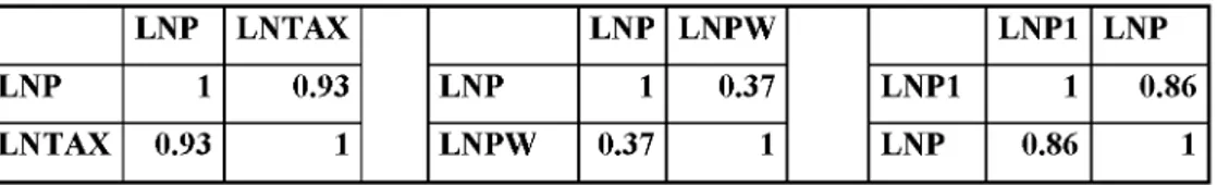
Table 4: Correlations between IVs and P t
LNP L N T A X L N P L N P W LNP1 LNP
LNP 1 0.93 LNP 1 0.37 LNP1 1 0.86
L N T A X 0.93 1 L N P W 0.37 1 LNP 0.86 1
Table 5: Correlations between IVs and Error terms
Resid1 L N T A X Resid1 L N P W Resid1 LNP1
Resid1 1.00 0.04 Resid1 1.00 0.00 Resid1 1.00 -0.19
L N T A X 0.04 1.00 L N P W 0.00 1.00 LNP1 -0.19 1.00
According to the correlation analysis, both IVs fulfill the necessary conditions, i.e. they are weakly correlated with the error terms of the initial specification, but highly correlated with the suspected variable, ln Pt. World oil price has
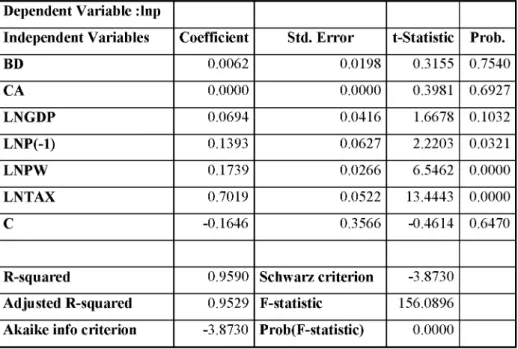
lower correlation (0.37) with lnPt than the other IVs, but it is uncorrelated with the residuals. As a result, including both IVs in the specification seems meaningful. In the next step, we regress ln Pt on the remaining regressors and on the IVs.
lnPt = (0 +0£At +(f>2BDt + (3 lnGDPt + j>4 l n Pt - 1 +(f>5 lnPWt + (6 lnTAXt
+ st (2)
The result of the previous equation is given in the following table;
Table 6: Endogeneity test, first specification
Dependent Variable :lnp
Independent Variables Coefficient Std. Error t-Statistic Prob.
BD 0.0062 0.0198 0.3155 0.7540 C A 0.0000 0.0000 0.3981 0.6927 L N G D P 0.0694 0.0416 1.6678 0.1032 LNP(-1) 0.1393 0.0627 2.2203 0.0321 L N P W 0.1739 0.0266 6.5462 0.0000 L N T A X 0.7019 0.0522 13.4443 0.0000 C -0.1646 0.3566 -0.4614 0.6470
R-squared 0.9590 Schwarz criterion -3.8730
Adjusted R-squared 0.9529 F-statistic 156.0896
Akaike info criterion -3.8730 Prob(F-statistic) 0.0000
According to the probability values, all of the IVs are statistically significant under 95% confidence interval. The remaining independent variables are statistically insignificant. Next step of the Hausman Test analysis is to run a second regression in which we re-estimate the initial equation including the residuals5 from equation 2.
Following is the output of the previous specification.
Table 7: Endogeneity test, second specification
Dependent Variable :LNQ
Independent Variables Coefficient Std. E r r o r t-Statistic Prob.
LNP -0.2144 0.2541 -0.8437 0.4037 BD 0.0630 0.0929 0.6784 0.5014 C A 0.0000 0.0002 -0.0667 0.9472 L N G D P 0.5487 0.2180 2.5167 0.0159 C 8.9733 1.8361 4.8870 0.0000 R E S I D 2 ( A4 ) 0.6213 0.8544 0.7272 0.4713
R-squared 0.1772 Schwarz criterion -0.3730
Adjusted R-squared 0.0769 F-statistic 1.7664
Akaike info criterion -0.6092 Prob(F-statistic) 0.1413
We will decide on whether there is an endogeneity problem in our specification and data by constructing the following hypothesis.
H0: The OLS estimates are consistent.6 (A4=0) HA: The OLS estimates are not consistent. (A4 ^0)
As the probability value of A4is equal to 0.4713, we fail to reject the null hypothesis. We can conclude that the OLS estimates are consistent. This result may not be correct since there are insignificant variables in the initial specification. For that reason, we will carry the endogeneity test after excluding insignificant CA and BD variables to be sure about the result. In our initial specification price is also insignificant, however as it is the main explanatory variable of the model, instead of omitting this variable, using appropriate lagged values might be a better solution. (Before the final specification, the lagged value(s) of the other insignificant variables will be investigated for their contribution to the model.)
6.1.2. Omitting Irrelevant Variables and Testing for Endogeneity
In this section, we will repeat the endogeneity test again. This time we will exclude the BD and CA variables, because in the final specification we will probably not use these variables since they are insignificant and do not contribute to R-square.
We will apply the same procedure like the previous section. The suspected variable and the instrumental variables are same. This time oil price and GDP are the explanatory variables. The result of the initial estimation is given in table 8.
ln Qt = J30 + P1 ln Pt + J32 ln GDPt + ut (4)
Table 8: Endogeneity test, initial specification
Dependent Variable :LNQ
Independent Variables Coefficient Std. E r r o r t-Statistic Prob.
LNP -0.2237 0.2194 -1.0196 0.3129
L N G D P 0.4348 0.2066 2.1046 0.0405
C 10.0534 1.7493 5.7469 0.0000
R-squared 0.0836 Schwarz criterion -0.3203
Adjusted R-squared 0.0462 F-statistic 2.2354
Akaike info criterion -0.4328 Prob(F-statistic) 0.1177
Then we regress ln Pt on the remaining regressors and on the IVs.
Table 9: Endogeneity test, first specification
Dependent Variable : LNP
Independent Variables Coefficient Std. Error t-Statistic Prob.
LNGDP 0.0780 0.0350 2.2288 0.0308
LNP1 0.1505 0.0555 2.7121 0.0094
LNPW 0.1741 0.0254 6.8587 0.0000
LNTAX 0.6848 0.0495 13.8293 0.0000
C -0.2411 0.3077 -0.7835 0.4373
R-squared 0.9555 Schwarz criterion -3.7617
Adjusted R-squared 0.9516 F-statistic 246.7484
Akaike info criterion -3.9511 Prob(F-statistic) 0.0000
All of the IVs are again statistically significant under 95% confidence interval. However, the signs of the IVs are not correct, for instance we expect the quantity demanded to decline while there is an increase in the taxation component. Next step is to run a second regression in which we re-estimate the initial equation including the residuals7 from the equation 5.
ln Qt = A0 + A ln Pt + A2GDPt +A3st + vt (6)
Table 10: Endogeneity test, second specification
Dependent Variable : LNP
Independent Variables Coefficient Std. Error t-Statistic Prob.
LNP 0.0780 0.2228 -1.2243 0.2269
LNGDP 0.1505 0.2117 1.7381 0.0887
R E S I D 3 0.1741 0.8856 0.8258 0.4131
C 0.6848 1.8010 6.0280 0.0000
R-squared 0.0674 Schwarz criterion -0.2970
Adjusted R-squared 0.0079 F-statistic 1.1340
By evaluating the same hypothesis, again we fail to reject the null hypothesis that the OLS estimates are consistent. As a result, there is no endogeneity problem after omitting the insignificant explanatory variables.
6.1.3. Seasonal adjustment
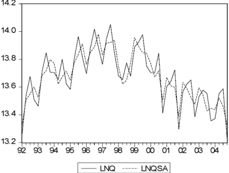
Economic time series based on monthly or quarterly data may exhibit seasonal patterns. In our case, gasoline consumption in summer may tend to increase because of travels to have holidays. It is often desirable to remove the seasonal factor to make series smoother. In this section, we will analyze i f the seasonal adjustment is necessary. Following figure illustrates the quantity series after and before the seasonal adjustment is performed. LNQSA is the seasonally adjusted series.
Figure 3: Seasonal Adjustment for Quantity Series
14.2 14.0 13.8 13.6 13.4 -13 2 " I 1 1 1 I 1 1 1 I 1 1 1 I 1 1 1 I 1 1 1 I 1 1 1 I 1 1 1 I 1 1 1 I 1 1 1 I 1 1 1 I 1 1 1 I 1 1 1 I 1 1 1 92 93 9 4 9 5 9 6 97 9 8 9 9 0 0 01 0 2 0 3 0 4 LNQ LNQSA
We decided that seasonal adjustment did not improve the data significantly, so we will use seasonally unadjusted series in our model. Quantity series are still non-stationary and have an increasing trend. Graphs for GDP and Price series are included in the appendix part.
5.3 Specifying Final Estimation
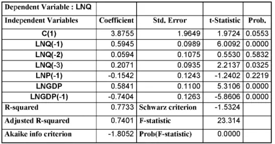
After evaluating different estimations due to their R-square, Schwarz and Akaike criterion, we decided the following auto-regressive distributed lag model to estimate the both short-run and long-run elasticities.
Table 11: Final Specification
Dependent Variable : LNQ
Independent Variables Coefficient Std. Error t-Statistic Prob.
C(1) 3.8755 1.9649 1.9724 0.0553 LNQ(-1) 0.5945 0.0989 6.0092 0.0000 LNQ(-2) 0.0594 0.1075 0.5530 0.5832 LNQ(-3) 0.2071 0.0935 2.2137 0.0325 LNP(-1) -0.1542 0.1243 -1.2402 0.2219 LNGDP 0.5841 0.1100 5.3106 0.0000 LNGDP(-I) -0.7404 0.1263 -5.8606 0.0000
R-squared 0.7733 Schwarz criterion -1.5324
Adjusted R-squared 0.7401 F-statistic 23.314
Akaike info criterion -1.8052 Prob(F-statistic) 0.0000
lnQt = 3,8755 - 0,1542lnP- 1 + 0,5945lnQ_x + 0,0594lnQ- 2
+ 0,2071ln Q- 3 + 0,5841ln GDP - 0,7404lnGDP_X (7)
In this final estimation, R-squared, 0.78, is quite good for our purposes.
5.4 Residual Test Result of the Final Specification
We performed the residual tests of the final specification in this section. White Heteroskedasticity test8 is employed to investigate whether the residuals of the regression have constant variance. F-statistics of the test is 0.813 and probability value is 0.637. We fail to reject the null hypothesis of there is no heteroskedasticity in 5% significance level. When we plot the residuals about the
zero line, we can see that residuals are stable in parameters of the equation except 1999.
Figure 4: Plot of Recursive Residuals
0.3 1 0.2¬ 0.1 -0.0¬ 0.1 0.2 -u - J 1 1 I 1 1 1 I 1 1 1 I 1 1 1 I 1 1 1 I 1 1 1 I 1 1 1 I 1 1 1 I 1 1 1 I 1 1 1 I 1 1 95 96 97 98 99 00 01 02 03 04 Recursive Residuals ± 2 S.E.
We use Breusch-Godfrey Serial Correlation L M Test9 and the F-statistics of the test is 0.1049 and probability value is 0.90. Again, we fail to reject the null hypothesis which means there is no serial correlation between the residuals.
5.5 Estimating Short-run and Long-run Elasticities
The coefficients of ln P- 1 and ln GDP show us the short-run elasticities.
Short-run price elasticity is equal to -0.15 and short-Short-run income elasticity is 0.58. However, short-run price elasticity is not statistically significant (p-value = 0.2219). We did not include ln P in our estimation since it did not contribute to R-square and was insignificant. In our analysis, quantity variable consists of the total of three months, so considering the coefficient of ln P- 1 (instead of ln P )
The long-run effect in an autoregressive distributed lag model is ^^_Qat where
at is the lagged terms' coefficient. The formulation of the lagged terms' coefficients are as the following;
1: at0 = ft> fwhlch will always be t h e case),
V: = ft o r « , = fa +a0r\,
L-: = fa o r a2 = + a0yz + « m ,
L3: —»oHa - - a
z^ + «s = & Or ffg = & 4- QqH + « 1 ft 4- GfcM,
L4: — « 1 ^ 3 - - «aW + a* = 0 o r « 4 = y^ctg + ytcti + ,
V: —atj-sys - « J - .zyz — ctj--\y\ -\- ctj = 0 o r ay = Kitty _i + > ï « y - 2 + H3«y-s. / = 5.6,
In our case J3t s are the coefficients of lag values of price, but only J31 is available which is equal to -0.15419. yt s are the coefficients of lag values of quantity and y1 = 0.5945 y2 = 0.0594 Y3= 0.2071. In the following table, the contribution of the each lag to the long-run equilibrium is given.
Table 12: Lag-coefficients of Long-run Price elasticity
Lagged term 1 2 3 4 5
Lag Coefficients -0.15 -0.09 -0.054 -0.047 -0.030
The long-run price elasticity of oil demand is equal to approximately -0.38. 15% of the long-run effect is coming from the first lagged term. This price elasticity is a plausible number for a developing country and consistent with the previous researches. The standard error of the long-run effect10 is equal to 0.18 and calculated t-statistics is equal to -2.23, so the long-run effect is significant at 5% significance level.
We will imply the same procedure to calculate the income elasticity of oil demand; this time J3t s are the coefficients of lag values of GDP.
1 0 The standard error of the long-run effect is the sum of the standard errors of the coefficients of
Table 13: Lag-coefficients of Long-run Income elasticity
Lagged term 0 1 2 3 4 5_ Lag Coefficients | 0.584 | -0.3931 -0.1991 -0.130 | -0.095 | -0.05
Long-term income elasticity is approximately -0.223. It is not a plausible number, because we expect a positive income elasticity. The standard error of the longrun income effect is equal to 0.17 and calculated tstatistics is equal to
7. C O N C L U S I O N
This thesis aims to reveal the magnitudes of both short-run and long-run income and price elasticities of gasoline consumption in Turkey. We are interested in this subject, because, as of the end of 2005, Turkey had the highest tax component in domestic oil prices among all European countries.
According to our findings, we estimate the shortrun price elasticity as -0.15, but this is not statistically significant. Short-run income elasticity is 0.58 and is statistically significant. It has a positive sign as expected. Our estimate of the long-run price elasticity is approximately -0.38 and we find the long-run income elasticity as approximately -0.223. Long-run price elasticity is statistically significant while long-run income elasticity is not.
Due to the income elasticity of oil demand, in the short-run, 1% increase in the real income level of public increases the oil consumption on average by 0.58%. However, it is not correct to use short-run income elasticity in policy-making.
By increasing the price of the oil derivative products 1%, government will lead to a reduction of approximately 0.38% of the quantity demanded. In that sense, oil tax level in Turkey seems not to be overly high. One reason of this relative inelasticity may be that since Turkey is a developing country that requires oil as a major input to generate its output, oil for the most part is consumed out of need and is therefore not a discretionary spending item. Moreover, oil has no close substitutes so whatever the price of the oil derivative products, in most of the industries, consumption remains nearly the same. This result is independent from the country-based elasticity but generally valid for developing countries. Another reason may be Turkey's geographic location. As it is the transportation center between Asia and Europe, foreign vehicles may be contributing significantly to oil consumption. However, we do not have data regarding this point.
Similar studies that are carried for other developing countries such as South Korea, Philippines and Taiwan indicate similar price elasticity numbers that varies between -0.30 and -0.60. However, in those countries, the tax component of oil price is smaller than it is in Turkey.
As a result, we advocate that price elasticity of oil demand for Turkey is as it is anticipated. According to the magnitude of this elasticity, tax component of oil price seems not suboptimal. However, the answer of this phenomenon will also depend on the magnitude of the distortions in the Turkish economy that oil taxation causes, but this is outside the scope of this thesis.
R E F E R E N C E S
Alves, D. & Bueno, R.L.S. (2003), 'Short-run, Long-run and Cross Elasticities of Gasoline Demand in Brazil, Energy Economics, vol. 25, pp. 191-199
Baltagi, B. H. & Griffin, J. M . (1983), 'Gasoline Demand in OECD: An Application of pooling and Testing Procedures', European Economic Review, vol. 22, pp. 117 - 137.
Central Bank of Turkey, 'data base', www.tcmb.gov.tr
Christopher, G. (1989), 'Gasoline, Diesel and Motor fuel Demand in Taiwan', Energy Journal vol. 10. pp. 153-63
Dahl, C. and Sterner, T. (1991), 'Analyzing gasoline demand elasticities: a survey', Energy Economics, vol.13, pp. 203-210
Dahl, C. and Sterner, T. (1991), 'A survey of econometric gasoline demand elasticities', International Journal of Energy Systems, vol. 11. pp. 53-76.
Enders, W. (2004), 'Applied Econometric Time Series' Second Edition, Wiley Series in Probability and Statistics, New Jersey
Gujarati, D. N . (1995), 'Basic Econometrics', Third Edition, Mc Graw Hill, Literature Press, Istanbul.
Goel, R. (1994), 'Quasi-experimental taxation elasticities of US gasoline demand, Energy Economics, vol.16, pp.133-137
Greene, W. H. (2003), 'Econometric Analysis', Fifth Edition, Prentice Hall, New Jersey
Henry, D. F. (2000), 'Econometrics: Alchemy or Science?, Essays in Econometric Methodology' Oxford University Press, Oxford, U K
Ibrahim, B. & Hurst, C. (1989), 'Estimating Energy and Oil Demand Functions: A Study of thirteen Developing Countries ', Energy Economics, vol. 12, pp. 93¬
102
International Energy Agency, 'Energy Policies of IEA Countries, Turkey 2001 Review'.
International Energy Agency Publications, (2004), 'Analysis of the Impact of High Oil Prices on the Global Economy'
Kennedy, M . (1974), 'An Economic Model of the World Oil Market', The Bell Journal of Economics and Management Science, vol. 5, pp. 540-577
Kennedy, P. (1996), 'A Guide to Econometrics' Third Edition, Blackwell Press, Oxford UK.
Kibritcioglu, A. & Kibritcioglu, B. (1999), 'Inflationary Effects of Increases in Prices of Imported Crude-Oil and Oil-Products in Turkey' Turkish Treasury Economic Research Department No. 21
Kirmanoglu, H. & Uyduranoglu, A. & Basjevent, C. (2003), 'The Effects of Tax on the Gasoline Consumption', V I . International Econometrics and Statistics Symposium, Gazi University
MacRae, R. (1994), ' Gasoline Demand in Developing Asian Countries', Energy Journal, vol. 15, issue 1
Mesutoglu,B. (2001), ' A Research on the Developments of Gasoline Price in Turkey and Price Elasticity of Gasoline Demand', Prime Ministry State Planning Organization of Turkey, ISBN 975.19.2689 - 0
Ramsey, J. & Rasche, R. & Bruce, T. (1975), 'An Analysis of the Private and Commercial Demand for Gasoline' Review of Economics & Statistics, vol. 57 pp. 502-07
Tupras Report, (2005) "The vision of Tupras"
Wasserfallen, W. & Guntensperger, H. (1988) 'Gasoline consumption and the stock of motor vehicle - An empirical analysis for the Swiss economy', Energy Economics, vol. 10. pp. 276-282.
'World Oil Market and Oil Price Chronologies: 1970 - 2004', Energy Information Administration, www.eia.doe.gov
Yürekli, A. & Wilkins, N . & Hu, T. (2004), 'Economic Analysis of Tobacco Demand, World Bank Economics of Tobacco Toolkit, Tool 3. Demand Analysis.
APPENDIX
Seasonal Adjustment for Price Series 3.4 3.2- 3.0- 2.8- 2.6-^ • 2.6-^ I I I I I I I I I I I I I I I I I I I I I I I I I I I I I I I I I I I I I I I I I I I I I I I I I I 9 2 9 3 9 4 9 5 9 6 97 9 8 9 9 0 0 01 0 2 0 3 0 4 LNPSA LNP
Seasonal Adjustment for GDP Series
10.2 10.0 9.8 9.6 9.4 . . . . . . . . . . . . . . . . . . . . . 92 93 94 95 96 97 98 99 00 01 02 03 04 LNGDP LNGDPSA
White Heteroskedasticity Test Output
White Heteroskedasticity Test:
F-statistic 0.812409 Probability 0.636339
Obs*R-squared 10.45719 Probability 0.575918
Dependent Variable: RESIDA2
Method: Least Squares Sample: 1992:4 2004:3 Included observations: 48
Variable Coefficient Std. Error t-Statistic Prob.
C -33.03283 19.87428 -1.662089 0.1054 LNQ(-1) 1.885835 1.331861 1.415940 0.1656 LNQ(-1)A2 -0.069520 0.048789 -1.424925 0.1630 LNQ(-2) 0.531027 1.220474 0.435098 0.6662 LNQ(-2)A2 -0.018604 0.044747 -0.415757 0.6801 LNQ(-3) 1.575094 1.177386 1.337789 0.1896 LNQ(-3)A2 -0.057837 0.043136 -1.340807 0.1886 LNP(-1) 0.409830 0.428303 0.956871 0.3452 LNP(-1)A2 -0.071799 0.073540 -0.976331 0.3356 LNGDP 1.070431 1.251197 0.855526 0.3981 LNGDPA2 -0.054458 0.063478 -0.857899 0.3968 LNGDP(-1) -0.037718 1.397074 -0.026998 0.9786 LNGDP(-1)A2 0.002889 0.070947 0.040719 0.9678
R-squared 0.217858 Mean dependent var 0.007192
Adjusted R-squared -0.050305 S.D.dependent var 0.010473
S.E. of regression 0.010733 Akaike info criterion -6.005084
Sum squared resid 0.004032 Schwarz criterion -5.498300
Log likelihood 157.1220 F-statistic 0.812409
Durbin-Watson stat 2.097518 Prob(F-statistic) 0.636339
Breusch-Godfrey Serial Correlation L M Test Output
Breusch-Godfrey Serial Correlation LM Test:
F-statistic 0.104965 Probability 0.900609
Obs*R-squared 0.256993 Probability 0.879417
Dependent Variable: RESID Method: Least Squares
Variable Coefficient Std. Error t-Statistic Prob.
C(1) -0.045606 2.033692 -0.022425 0.9822 LNQ(-1) -0.039948 0.138482 -0.288470 0.7745 LNQ(-2) 0.020475 0.135339 0.151290 0.8805 LNQ(-3) 0.006632 0.109656 0.060479 0.9521 LNP(-1) -0.021295 0.146261 -0.145598 0.8850 LNGDP 0.008565 0.114165 0.075020 0.9406 LNGDP(-1) 0.020260 0.149896 0.135161 0.8932 RESID(-1) 0.097134 0.214442 0.452959 0.6531 RESID(-2) -0.000621 0.227649 -0.002726 0.9978
R-squared 0.005354 Mean dependent var 1.51E-15
Adjusted R-squared -0.198676 S.D. dependent var 0.085701
S.E. of regression 0.093829 Akaike info criterion -1.727318
Sum squared resid 0.343354 Schwarz criterion -1.376468
Log likelihood 50.45564 F-statistic 0.026241