arXiv:1504.02680v3 [hep-ex] 2 Jun 2015
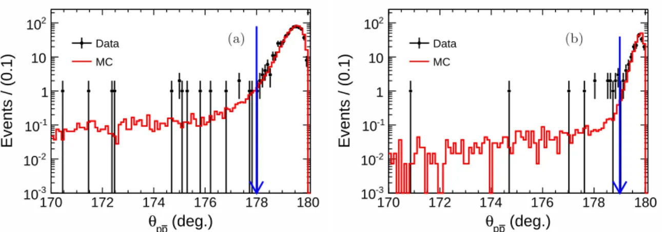
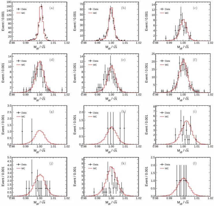
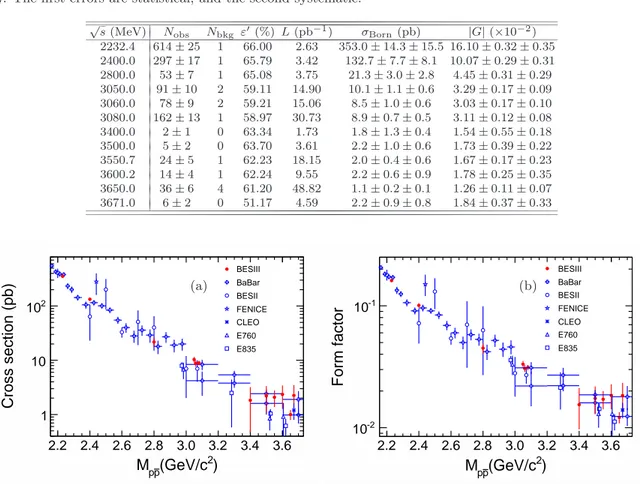
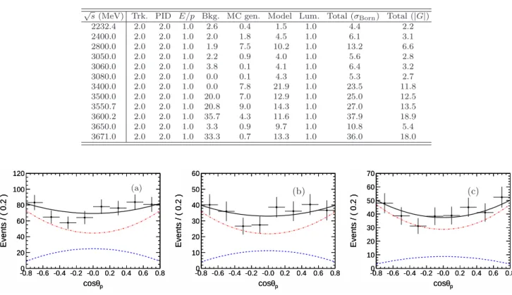
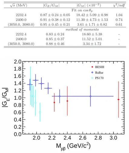
Measurement of the proton form factor by studying e
+e
−→ p
p
¯
M. Ablikim1, M. N. Achasov9,a, X. C. Ai1, O. Albayrak5, M. Albrecht4, D. J. Ambrose44, A. Amoroso48A,48C, F. F. An1, Q. An45, J. Z. Bai1, R. Baldini Ferroli20A, Y. Ban31, D. W. Bennett19, J. V. Bennett5, M. Bertani20A, D. Bettoni21A, J. M. Bian43, F. Bianchi48A,48C, E. Boger23,h, O. Bondarenko25, I. Boyko23, R. A. Briere5, H. Cai50, X. Cai1, O. Cakir40A,b,
A. Calcaterra20A, G. F. Cao1, S. A. Cetin40B, J. F. Chang1, G. Chelkov23,c, G. Chen1, H. S. Chen1, H. Y. Chen2, J. C. Chen1, M. L. Chen1, S. J. Chen29, X. Chen1, X. R. Chen26, Y. B. Chen1, H. P. Cheng17, X. K. Chu31, G. Cibinetto21A,
D. Cronin-Hennessy43, H. L. Dai1, J. P. Dai34, A. Dbeyssi14, D. Dedovich23, Z. Y. Deng1, A. Denig22, I. Denysenko23, M. Destefanis48A,48C, F. De Mori48A,48C, Y. Ding27, C. Dong30, J. Dong1, L. Y. Dong1, M. Y. Dong1, S. X. Du52, P. F. Duan1, J. Z. Fan39, J. Fang1, S. S. Fang1, X. Fang45, Y. Fang1, L. Fava48B,48C, F. Feldbauer22, G. Felici20A, C. Q. Feng45, E. Fioravanti21A, M. Fritsch14,22, C. D. Fu1, Q. Gao1, X. Y. Gao2, Y. Gao39, Z. Gao45, I. Garzia21A, C. Geng45, K. Goetzen10, W. X. Gong1, W. Gradl22, M. Greco48A,48C, M. H. Gu1, Y. T. Gu12, Y. H. Guan1, A. Q. Guo1, L. B. Guo28, Y. Guo1, Y. P. Guo22, Z. Haddadi25, A. Hafner22, S. Han50, Y. L. Han1, X. Q. Hao15, F. A. Harris42, K. L. He1,
Z. Y. He30, T. Held4, Y. K. Heng1, Z. L. Hou1, C. Hu28, H. M. Hu1, J. F. Hu48A,48C, T. Hu1, Y. Hu1, G. M. Huang6, G. S. Huang45, H. P. Huang50, J. S. Huang15, X. T. Huang33, Y. Huang29, T. Hussain47, Q. Ji1, Q. P. Ji30, X. B. Ji1, X. L. Ji1, L. L. Jiang1, L. W. Jiang50, X. S. Jiang1, J. B. Jiao33, Z. Jiao17, D. P. Jin1, S. Jin1, T. Johansson49, A. Julin43,
N. Kalantar-Nayestanaki25, X. L. Kang1, X. S. Kang30, M. Kavatsyuk25, B. C. Ke5, R. Kliemt14, B. Kloss22, O. B. Kolcu40B,d, B. Kopf4, M. Kornicer42, W. K¨uhn24, A. Kupsc49, W. Lai1, J. S. Lange24, M. Lara19, P. Larin14, C. Leng48C, C. H. Li1, Cheng Li45, D. M. Li52, F. Li1, G. Li1, H. B. Li1, J. C. Li1, Jin Li32, K. Li13, K. Li33, Lei Li3, P. R. Li41, T. Li33, W. D. Li1, W. G. Li1, X. L. Li33, X. M. Li12, X. N. Li1, X. Q. Li30, Z. B. Li38, H. Liang45, Y. F. Liang36,
Y. T. Liang24, G. R. Liao11, D. X. Lin14, B. J. Liu1, C. X. Liu1, F. H. Liu35, Fang Liu1, Feng Liu6, H. B. Liu12, H. H. Liu1, H. H. Liu16, H. M. Liu1, J. Liu1, J. P. Liu50, J. Y. Liu1, K. Liu39, K. Y. Liu27, L. D. Liu31, P. L. Liu1, Q. Liu41, S. B. Liu45,
X. Liu26, X. X. Liu41, Y. B. Liu30, Z. A. Liu1, Zhiqiang Liu1, Zhiqing Liu22, H. Loehner25, X. C. Lou1,e, H. J. Lu17, J. G. Lu1, R. Q. Lu18, Y. Lu1, Y. P. Lu1, C. L. Luo28, M. X. Luo51, T. Luo42, X. L. Luo1, M. Lv1, X. R. Lyu41, F. C. Ma27,
H. L. Ma1, L. L. Ma33, Q. M. Ma1, S. Ma1, T. Ma1, X. N. Ma30, X. Y. Ma1, F. E. Maas14, M. Maggiora48A,48C, Q. A. Malik47, Y. J. Mao31, Z. P. Mao1, S. Marcello48A,48C, J. G. Messchendorp25, J. Min1, T. J. Min1, R. E. Mitchell19, X. H. Mo1, Y. J. Mo6, C. Morales Morales14, K. Moriya19, N. Yu. Muchnoi9,a, H. Muramatsu43, Y. Nefedov23, F. Nerling14,
I. B. Nikolaev9,a, Z. Ning1, S. Nisar8, S. L. Niu1, X. Y. Niu1, S. L. Olsen32, Q. Ouyang1, S. Pacetti20B, P. Patteri20A, M. Pelizaeus4, H. P. Peng45, K. Peters10, J. Pettersson49, J. L. Ping28, R. G. Ping1, R. Poling43, Y. N. Pu18, M. Qi29, S. Qian1, C. F. Qiao41, L. Q. Qin33, N. Qin50, X. S. Qin1, Y. Qin31, Z. H. Qin1, J. F. Qiu1, K. H. Rashid47, C. F. Redmer22,
H. L. Ren18, M. Ripka22, G. Rong1, X. D. Ruan12, V. Santoro21A, A. Sarantsev23,f, M. Savri´e21B, K. Schoenning49, S. Schumann22, W. Shan31, M. Shao45, C. P. Shen2, P. X. Shen30, X. Y. Shen1, H. Y. Sheng1, W. M. Song1, X. Y. Song1,
S. Sosio48A,48C, S. Spataro48A,48C, G. X. Sun1, J. F. Sun15, S. S. Sun1, Y. J. Sun45, Y. Z. Sun1, Z. J. Sun1, Z. T. Sun19, C. J. Tang36, X. Tang1, I. Tapan40C, E. H. Thorndike44, M. Tiemens25, D. Toth43, M. Ullrich24, I. Uman40B, G. S. Varner42,
B. Wang30, B. L. Wang41, D. Wang31, D. Y. Wang31, K. Wang1, L. L. Wang1, L. S. Wang1, M. Wang33, P. Wang1, P. L. Wang1, Q. J. Wang1, S. G. Wang31, W. Wang1, X. F. Wang39, Y. D. Wang20A, Y. F. Wang1, Y. Q. Wang22, Z. Wang1,
Z. G. Wang1, Z. H. Wang45, Z. Y. Wang1, T. Weber22, D. H. Wei11, J. B. Wei31, P. Weidenkaff22, S. P. Wen1, U. Wiedner4, M. Wolke49, L. H. Wu1, Z. Wu1, L. G. Xia39, Y. Xia18, D. Xiao1, Z. J. Xiao28, Y. G. Xie1, Q. L. Xiu1, G. F. Xu1, L. Xu1, Q. J. Xu13, Q. N. Xu41, X. P. Xu37, L. Yan45, W. B. Yan45, W. C. Yan45, Y. H. Yan18, H. X. Yang1, L. Yang50, Y. Yang6,
Y. X. Yang11, H. Ye1, M. Ye1, M. H. Ye7, J. H. Yin1, B. X. Yu1, C. X. Yu30, H. W. Yu31, J. S. Yu26, C. Z. Yuan1, W. L. Yuan29, Y. Yuan1, A. Yuncu40B,g, A. A. Zafar47, A. Zallo20A, Y. Zeng18, B. X. Zhang1, B. Y. Zhang1, C. Zhang29,
C. C. Zhang1, D. H. Zhang1, H. H. Zhang38, H. Y. Zhang1, J. J. Zhang1, J. L. Zhang1, J. Q. Zhang1, J. W. Zhang1, J. Y. Zhang1, J. Z. Zhang1, K. Zhang1, L. Zhang1, S. H. Zhang1, X. Y. Zhang33, Y. Zhang1, Y. H. Zhang1, Y. T. Zhang45,
Z. H. Zhang6, Z. P. Zhang45, Z. Y. Zhang50, G. Zhao1, J. W. Zhao1, J. Y. Zhao1, J. Z. Zhao1, Lei Zhao45, Ling Zhao1, M. G. Zhao30, Q. Zhao1, Q. W. Zhao1, S. J. Zhao52, T. C. Zhao1, Y. B. Zhao1, Z. G. Zhao45, A. Zhemchugov23,h, B. Zheng46,
J. P. Zheng1, W. J. Zheng33, Y. H. Zheng41, B. Zhong28, L. Zhou1, Li Zhou30, X. Zhou50, X. K. Zhou45, X. R. Zhou45, X. Y. Zhou1, K. Zhu1, K. J. Zhu1, S. Zhu1, X. L. Zhu39, Y. C. Zhu45, Y. S. Zhu1, Z. A. Zhu1, J. Zhuang1, L. Zotti48A,48C,
B. S. Zou1, J. H. Zou1 (BESIII Collaboration)
1 Institute of High Energy Physics, Beijing 100049, People’s Republic of China 2 Beihang University, Beijing 100191, People’s Republic of China
3 Beijing Institute of Petrochemical Technology, Beijing 102617, People’s Republic of China 4 Bochum Ruhr-University, D-44780 Bochum, Germany
5 Carnegie Mellon University, Pittsburgh, Pennsylvania 15213, USA 6 Central China Normal University, Wuhan 430079, People’s Republic of China
7 China Center of Advanced Science and Technology, Beijing 100190, People’s Republic of China
8 COMSATS Institute of Information Technology, Lahore, Defence Road, Off Raiwind Road, 54000 Lahore, Pakistan 9 G.I. Budker Institute of Nuclear Physics SB RAS (BINP), Novosibirsk 630090, Russia
10GSI Helmholtzcentre for Heavy Ion Research GmbH, D-64291 Darmstadt, Germany 11 Guangxi Normal University, Guilin 541004, People’s Republic of China
12 GuangXi University, Nanning 530004, People’s Republic of China 13 Hangzhou Normal University, Hangzhou 310036, People’s Republic of China
14 Helmholtz Institute Mainz, Johann-Joachim-Becher-Weg 45, D-55099 Mainz, Germany 15 Henan Normal University, Xinxiang 453007, People’s Republic of China
16 Henan University of Science and Technology, Luoyang 471003, People’s Republic of China 17Huangshan College, Huangshan 245000, People’s Republic of China
18Hunan University, Changsha 410082, People’s Republic of China 19 Indiana University, Bloomington, Indiana 47405, USA
20(A)INFN Laboratori Nazionali di Frascati, I-00044, Frascati, Italy; (B)INFN and University of Perugia, I-06100, Perugia, Italy
21 (A)INFN Sezione di Ferrara, I-44122, Ferrara, Italy; (B)University of Ferrara, I-44122, Ferrara, Italy 22Johannes Gutenberg University of Mainz, Johann-Joachim-Becher-Weg 45, D-55099 Mainz, Germany
23 Joint Institute for Nuclear Research, 141980 Dubna, Moscow region, Russia
24 Justus Liebig University Giessen, II. Physikalisches Institut, Heinrich-Buff-Ring 16, D-35392 Giessen, Germany 25 KVI-CART, University of Groningen, NL-9747 AA Groningen, The Netherlands
26Lanzhou University, Lanzhou 730000, People’s Republic of China 27Liaoning University, Shenyang 110036, People’s Republic of China 28 Nanjing Normal University, Nanjing 210023, People’s Republic of China
29 Nanjing University, Nanjing 210093, People’s Republic of China 30Nankai University, Tianjin 300071, People’s Republic of China
31 Peking University, Beijing 100871, People’s Republic of China 32Seoul National University, Seoul, 151-747 Korea 33Shandong University, Jinan 250100, People’s Republic of China 34Shanghai Jiao Tong University, Shanghai 200240, People’s Republic of China
35 Shanxi University, Taiyuan 030006, People’s Republic of China 36 Sichuan University, Chengdu 610064, People’s Republic of China
37 Soochow University, Suzhou 215006, People’s Republic of China 38Sun Yat-Sen University, Guangzhou 510275, People’s Republic of China
39Tsinghua University, Beijing 100084, People’s Republic of China
40 (A)Istanbul Aydin University, 34295 Sefakoy, Istanbul, Turkey; (B)Dogus University, 34722 Istanbul, Turkey; (C)Uludag University, 16059 Bursa, Turkey
41 University of Chinese Academy of Sciences, Beijing 100049, People’s Republic of China 42 University of Hawaii, Honolulu, Hawaii 96822, USA
43 University of Minnesota, Minneapolis, Minnesota 55455, USA 44University of Rochester, Rochester, New York 14627, USA
45 University of Science and Technology of China, Hefei 230026, People’s Republic of China 46 University of South China, Hengyang 421001, People’s Republic of China
47 University of the Punjab, Lahore-54590, Pakistan
48 (A)University of Turin, I-10125, Turin, Italy; (B)University of Eastern Piedmont, I-15121, Alessandria, Italy; (C)INFN, I-10125, Turin, Italy
49 Uppsala University, Box 516, SE-75120 Uppsala, Sweden 50Wuhan University, Wuhan 430072, People’s Republic of China 51Zhejiang University, Hangzhou 310027, People’s Republic of China 52Zhengzhou University, Zhengzhou 450001, People’s Republic of China
a Also at the Novosibirsk State University, Novosibirsk, 630090, Russia bAlso at Ankara University, 06100 Tandogan, Ankara, Turkey
c Also at the Moscow Institute of Physics and Technology, Moscow 141700, Russia and at the Functional Electronics Laboratory, Tomsk State University, Tomsk, 634050, Russia
dCurrently at Istanbul Arel University, 34295 Istanbul, Turkey e Also at University of Texas at Dallas, Richardson, Texas 75083, USA f Also at the NRC ”Kurchatov Institute”, PNPI, 188300, Gatchina, Russia
g Also at Bogazici University, 34342 Istanbul, Turkey
hAlso at the Moscow Institute of Physics and Technology, Moscow 141700, Russia
1
1
(Dated: June 3, 2015)
Using data samples collected with the BESIII detector at the BEPCII collider, we measure the Born cross section of e+e− → p¯p at 12 center-of-mass energies from 2232.4 to 3671.0 MeV. The corresponding effective electromagnetic form factor of the proton is deduced under the assumption that the electric and magnetic form factors are equal (|GE| = |GM|). In addition, the ratio of electric
to magnetic form factors, |GE/GM|, and |GM| are extracted by fitting the polar angle distribution of the proton for the data samples with larger statistics, namely at √s = 2232.4 and 2400.0 MeV and a combined sample at√s = 3050.0, 3060.0 and 3080.0 MeV, respectively. The measured cross sections are in agreement with recent results from BaBar, improving the overall uncertainty by about 30%. The |GE/GM| ratios are close to unity and consistent with BaBar results in the same q2
region, which indicates the data are consistent with the assumption that |GE| = |GM| within uncertainties.
PACS numbers: 13.66.Bc, 14.20.Dh, 13.40.Gp
I. INTRODUCTION
Electromagnetic form factors (FFs) of the nucleon pro-vide fundamental information about its internal struc-ture and dynamics. They constitute a rigorous test of non-perturbative QCD as well as of phenomenological models.
Proton FFs can be measured in different kinematic re-gions by i) lepton-proton elastic scattering (space-like, la-beled SL) ii) electron-positron annihilation into a proton-antiproton pair or proton-proton-antiproton annihilation into an electron-positron (time-like, labeled TL). The low-est order Feynman diagram of lepton-proton scattering
is shown in Fig.1(a). The momentum transfer squared,
q2, is negative and the FFs are real functions of q2.
The lowest order e+e− annihilation process is shown in
Fig.1(b). Here, q2 is positive and the FFs are complex
functions of q2. The basic kinematic variables are also
shown in Fig.1, where k, k′ are the initial and final
elec-tron momenta and p, p′ are the initial and final proton
momenta. Since the electromagnetic vertex of the lepton is well known, one can reliably extract the proton
electro-magnetic vertex Γµ by measuring the cross section and
the polarization. Assuming one-photon exchange, i.e. in Born approximation, and under the basic requirements of Lorentz invariance, the hadronic vertex can be
param-eterized in terms of two FFs, F1 and F2 [1],
Γµ(p′, p) = γµF1(q2) +
iσµνqν
2mp
κpF2(q2), (1)
where the element σµν = γµγν − γνγµ is a
representa-tion of the Lorentz group, mp is the mass of the proton,
κp = gp2−2 is the anomalous magnetic moment of the
proton, gp = µJp, µp = 2.79 is the magnetic moment of
the proton and J = 1
2 is its spin. The functions F1 and
F2 are the so called Dirac and Pauli FFs, respectively.
The optical theorem, applied to lepton-nucleon scatter-ing, implies that at the lowest order the FFs are real in
the SL region [2] [3], i.e. the complex conjugate of the
amplitude in Fig.1(a), M†, is identical to M. In the TL
region, as in in Fig.1(b), the FFs can be complex above
the first hadronic threshold, that is, above twice the pion mass.
The Sachs FFs, electric GE and magnetic GM, are
introduced as linear combinations of the Dirac and Pauli
FFs [4]. Concerning the SL region in the Breit frame, GE
and GM are the Fourier transforms of the charge and
magnetization distribution of the nucleon, respectively.
GM and GE are proportional to flip and non
spin-flip amplitudes, respectively. They are expressed as
GE(q2) = F1(q2) + q 2 4m2 p κpF2(q2), (2) GM(q2) = F1(q2) + κpF2(q2). (3)
In the TL region, the center-of-mass (c.m.) system is equivalent to the Breit frame since the helicities of
baryons are opposite for the spinors aligned in GM and
are the same for the spinors aligned in GE.
In the SL region, FFs have been extracted by the
Rosenbluth separation method [5], as well as, more
recently, by the recoil proton polarization transfer
method [6]. The latter has been applied to obtain the
µpGE/GM ratio. Results from the GEp-II experiment
at JLab’s Hall A [7,8] for µpGE/GM show that this
ra-tio decreases rather quickly with increasing Q2, where
Q2= −q2≥ 0, while results achieved by the Rosenbluth
method show an almost constant ratio [9]. The
discrep-ancy between the Rosenbluth and the polarization trans-fer method may be resolved by including higher order corrections like two-photon exchange. A small correction to the Rosenbluth separation could imply a large
correc-tion for the extraccorrec-tion of GE, since GE is the slope of
the Rosenbluth plot. However, the correction of includ-ing two-photon exchange is small and cannot significantly influence the results of the polarization transfer experi-ment.
In the TL region, measurements have been performed
in the direct production channel e+e− → p¯p [10–14], in
the radiative return channel e+e− → p¯p(γ
ISR) [15, 16]
where γISR refers to a photon emitted by initial state
radiation (ISR), and in ¯pp → e+e− [17–19] experiments.
In cases where the data sample is too small to extract
an-gular distributions and disentangle |GE| and |GM|, the
effective proton FF |G| can be calculated from the
to-tal cross section, assuming |GE| = |GM|. This
assump-tion is valid at the p¯p mass threshold, if analyticity of
the FFs holds, implying that at threshold the angular distribution should be isotropic. In the PS170
exper-iment at LEAR [17], the effective proton FF was
ob-tained, as well as the |GE/GM| ratio, from p¯p threshold
up to√s = 2.05 GeV. In the BaBar experiment at
-e e -) k , e =(E µ k k’µ=(E’e, k’) |e> µ γ =<e’| µ j * γ q2<0 p p ) p , p =(E µ P P’µ=(E’p, p’) (p’,p)|p> µ Γ =<p’| µ J (a) -e + e ) k , e =(E µ k ) k’ , e =(E’ µ k’ |e> µ γ =<e’| µ j * γ >0 2 q p p ) p , p =(E µ P ) p’ , p =(E’ µ P’ (p’,p)|p> µ Γ =<p’| µ J (b)
FIG. 1. (a) Feynman diagram of ep → ep elastic scattering at the lowest order. (b) Feynman diagram of e+e− → p¯p annihilation at the lowest order (identical to that of the reverse reaction p¯p → e+e− with e ↔ p exchange.)
method from the p¯p production threshold up to√s = 6.5
GeV. The |GE/GM| ratio was measured from threshold
up to √s = 3.0 GeV and the result shows an
inconsis-tency with respect to the PS170 results.
The presence of vector resonances, like ρ, ω and φ in
the unphysical region, below the p¯p threshold, can
in-fluence the functional form of the FFs in the physical
region. Hence the FFs, in particular the ratio |GE/GM|,
in the TL region cannot be simply extrapolated from the SL ones. Until now it has been assumed that all FFs respect analyticity, which should allow to calculate their behavior in the unphysical region thanks to dispersion
re-lations [20] using the available data in both the TL and
SL regions. In the SL region, the ratio µpGE/GM has
been measured at 16 Q2 values in (0.5, 8.5) GeV2 with
the best precision to 1.7% [7, 8], while the present
pre-cision of |GE/GM| in the TL region exceeds 10% by far.
Therefore, it is necessary to improve the measurement of
|GE/GM| ratio in the TL region.
The experimental determinations of proton FFs are important input for various QCD-based theoretical mod-els. There are plenty of theoretical approaches applied to
explain TL FFs: Chiral Perturbation Theory [21], Lattice
QCD [22] [23], Vector Meson Dominance (VMD) [24], the
Relativistic Constituent Quark Model (CQM) [25], and,
at high energies, perturbative QCD predictions [26].
In this paper, we present an investigation of the process
e+e−→ p¯p based on data samples collected with the
Bei-jing Spectrometer III (BESIII) [27] at the Beijing
Elec-tron PosiElec-tron Collider II (BEPCII) at 12 c.m. energies
(√s). The Born cross section at these energy points are
measured and the corresponding effective FFs are
deter-mined. The ratio of electric to magnetic FFs, |GE/GM|,
and |GM| are measured at those c.m. energies where the
statistics are large enough. The results are consistent
with those from BaBar in the same q2 region.
II. THE BESIII EXPERIMENT AND DATA
SETS
BEPCII is a double-ring e+e− collider running at
c.m. energies between 2.0-4.6 GeV and reached a peak
luminosity of 0.85 × 1033cm−2s−1 at a c.m. energy of
3770 MeV. The cylindrical BESIII detector has an effec-tive geometrical acceptance of 93% of 4π and is divided into a barrel section and two endcaps. It contains a small
cell, helium-based (40% He, 60% C3H8) main drift
cham-ber (MDC) which provides momentum measurement for charged particles with a resolution of 0.5% at a momen-tum of 1 GeV/c in a magnetic field of 1 Tesla. The energy loss measurement (dE/dx) provided by the MDC has a resolution better than 6%. A time-of-flight system (TOF) consisting of 5-cm-thick plastic scintillators can measure the flight time of charged particles with a time resolution of 80 ps in the barrel and 110 ps in the end-caps. An electromagnetic calorimeter (EMC) consisting of 6240 CsI (Tl) in a cylindrical structure and two end-caps is used to measure the energies of photons and elec-trons. The energy resolution of the EMC is 2.5% in the barrel and 5.0% in the end-caps for photon/electron of 1 GeV energy. The position resolution of the EMC is 6 mm in the barrel and 9 mm in the end caps. A muon system
(MUC) consisting of about 1000 m2 of Resistive Plate
Chambers (RPC) is used to identify muons and provides a spatial resolution better than 2 cm.
Monte Carlo (MC) simulated signal and background samples are used to optimize the event selection crite-ria, estimate the background contamination and evalu-ate the selection efficiencies. The MC samples are
gen-erated using a Geant4-based [28] simulation software
package BESIII Object Oriented Simulation Tool
(BOOST) [29], which includes the description of
geom-etry and material, the detector response and the dig-itization model, as well as a database of the detector running conditions and performances. In this analysis,
the generator software package Conexc [30] is used to
simulate the signal MC samples e+e− → p¯p, and
cal-culate the corresponding correction factors for higher order process with one radiative photon in the final
cross check of the radiative correction factors. At each c.m. energy, a large signal MC sample with more than 10 times of the produced events in data for the process
e+e− → p¯p, contributing 0.15% statistical uncertainty
on the detection efficiency, is generated. Simulated
sam-ples of the QED background processes e+e− → l+l− (l
= e, µ) and e+e− → γγ are generated with the
genera-tor Babayaga [32]. The other background MC samples
for the processes with the hadronic final states e+e− →
h+h− (h = π, K), e+e− → p¯pπ0, e+e− → p¯pπ0π0 and
e+e−→ Λ¯Λ are generated with uniform phase space
dis-tributions. The background samples are generated with equivalent luminosities at least as large as the data sam-ples.
III. ANALYSIS STRATEGY
A. Event selection
Charged tracks are reconstructed with the hit informa-tion from the MDC. A good charged track must be within the MDC coverage, | cos θ| < 0.93, and is required to pass
within 1 cm of the e+e− interaction point (IP) in the
plane perpendicular to the beam and within ±10 cm in the direction along the beam. The combined information of dE/dx and TOF is used to calculate particle identifi-cation (PID) probabilities for the pion, kaon and proton hypothesis, respectively, and the particle type with the highest probability is assigned to the track. In this anal-ysis, exactly two good charged tracks, one proton and one antiproton, are required. To suppress Bhabha back-ground events, the ratio E/p of each proton candidate is required to be smaller than 0.5, where E and p are the en-ergy deposited in the EMC and the momentum measured in the MDC, respectively. The cosmic ray background is
rejected by requiring |Ttrk1− Ttrk2| <4 ns, where Ttrk1
and Ttrk2 are the measured time of flight in the TOF
detector for the two tracks. For the samples with c.m.
energy√s > 2400.0 MeV, the proton is further required
to satisfy cos θ < 0.8 to suppress Bhabha background. After applying the above selection criteria, the distri-butions of the opening angle between proton and
an-tiproton, θp ¯p, at c.m. energies √s = 2232.4 and 3080.0
MeV are shown in Fig. 2. Good agreement between
data and MC samples is observed, and a better reso-lution is achieved with increasing c.m. energy due to the smaller effects on the small angle multiple scattering. A
c.m. energy dependent requirement, i.e., θp ¯p > 178◦ at
√
s ≤ 2400.0 MeV, and θp ¯p> 179◦at√s > 2400.0 MeV,
is further applied. Figure 3 shows the distribution of
the momentum of proton or antiproton at c.m. energies √
s = 2232.4 and 3080.0 MeV. A momentum window of
5 times the momentum resolution, |pmea− pexp| < 5σp,
is applied to extract the signals, where pmeaand pexp are
the measured and expected momentum of the proton or
antiproton in the c.m. system, respectively, and σpis the
corresponding resolution.
B. Background study
The potential background contamination can be classi-fied into two categories, the beam associated background and the physical background.
The beam associated background includes interactions between the beam and the beam pipe, beam and
resid-ual gas, and the Touschek effect [33]. Dedicated data
samples with separated beams were collected with the
BESIII detector at√s = 2400.0 and 3400.0 MeV; these
are used to study the beam associated background. Since the two beams do not interact with each other, all of the observed events are beam associated background, and can be used to evaluate the beam associated background at different c.m. energies by normalizing the data-taking time and efficiencies. No events from the separated beam data samples survive the signal selection criteria. Con-sidering that the normalization factor is less than 5 for most of energy points (other than 3.08 and 3.65 GeV), the beam associated background at all c.m. energy points is negligible.
The physical background may come from the e+e−
annihilation processes with two-body final states, e.g. Bhabha or di-muon events, where leptons are misiden-tified as protons or antiprotons, or processes with
multi-body final states including p¯p, e.g. e+e− → p¯pπ0(π0).
The contamination from physical background is
eval-uated by MC samples, and are listed in Table I for
√
s = 2232.4 and 3080.0 MeV, respectively.
The number of the surviving background events after
normalization, NMC
nor, is very small at the low c.m.
en-ergies and can therefore be safely neglected. However,
at higher c.m. energies (√s ≥ 3.40 GeV), due to the
rapid decrease of the cross section of e+e− → p¯p, the
background level which is mainly from Bhabha events is
higher, and NnorMC needs to be corrected for.
The ratio of p¯p invariant mass and the c.m. energy,
Mp ¯p/√s, from data and MC has been compared and is
shown in Fig. 4 at different c.m. energies. The integral
luminosity of the data set at each c.m. energy is listed in
TableII. There is good agreement between data and MC
simulations. The signal yields are extracted by counting
the number of events and are listed in Table II, where
the quoted uncertainties are statistical only. The data sample at 3550.7 MeV is a combination of three data
sub-samples with very close c.m. energies,√s = 3542.4,
3553.8, 3561.1 MeV, and the value of 3550.7 MeV is the average c.m. energy weighted with their luminosity val-ues.
(deg.) p p θ 170 172 174 176 178 180 Events / (0.1) -3 10 -2 10 -1 10 1 10 2 10 Data MC (a) (deg.) p p θ 170 172 174 176 178 180 Events / (0.1) -3 10 -2 10 -1 10 1 10 2 10 Data MC (b)
FIG. 2. Opening angle distributions between proton and antiproton at the c.m. energies of (a) 2232.4 MeV, and (b) 3080.0 MeV. The dots with error bars are data, the histograms represent the distributions of signal MC samples. The arrows show the selection applied.
(GeV/c) p p / p 0.55 0.60 0.65 0.70 Events / (3.0 MeV/c) 0 100 200 300 400 Data MC (a) (GeV/c) p p / p 1.15 1.20 1.25 1.30 Events / (3.0 MeV/c) 0 20 40 60 Data MC (b)
FIG. 3. Momentum distribution of the proton or antiproton at the c.m. energies (a) 2232.4 MeV, and (b) 3080.0 MeV, two entries per event. The dots with error bars are data, the histograms represent the distributions of signal MC samples. The arrows show the momentum window requirements.
TABLE I. Physical background processes estimated from the MC samples at√s = 2232.4 and 3080.0 MeV. NMC
gen is the number of generated MC events, NMC
sur is the number of events remaining after the selection criteria, σ is the production cross section in the e+e−annihilation process, which is obtained using the Babayaga generator for Bhabha, di-muon, and di-photon processes, and from the previous experimental results for others processes [34, 35]. NMC
uplimit and N MC
nor are the estimated upper limit at the 90% confidence level (C.L.) and the normalized number of background events.
√s = 2232.4 MeV (2.63 pb−1) √s = 3080.0 MeV (30.73 pb−1) Bkg. NMC
gen (×106) NsurMC σ (nb) NuplimitMC NnorMC NgenMC(×106) NsurMC σ (nb) NuplimitMC NnorMC
e+e− 9.6 0 1435.01 < 0.96 0 39.9 1 756.86 < 2.54 1 µ+µ− 0.7 0 17.41 < 0.16 0 1.5 0 8.45 < 0.42 0 γγ 1.9 0 70.44 < 0.24 0 4.5 0 37.05 < 0.62 0 π+π− 0.1 0 0.17 < 0.01 0 0.1 0 < 0.11 < 0.02 0 K+K− 0.1 0 0.14 < 0.008 0 0.1 0 0.093 < 0.02 0 p¯pπ0 0.1 0 < 0.1 < 0.006 0 0.1 0 < 0.1 < 0.07 0 p¯pπ0π0 0.1 0 < 0.1 < 0.006 0 0.1 0 < 0.1 < 0.07 0 ΛΛ 0.1 0 < 0.4 < 0.02 0 0.1 0 0.002 < 0.001 0
s / p p M 0.98 0.99 1.00 1.01 1.02 Event / 0.001 0 20 40 60 80 100 120 140 160 180 Data MC (a) s / p p M 0.98 0.99 1.00 1.01 1.02 Event / 0.001 0 10 20 30 40 50 60 70 Data MC (b) s / p p M 0.98 0.99 1.00 1.01 1.02 Event / 0.001 0 2 4 6 8 10 12 14 Data MC (c) s / p p M 0.98 0.99 1.00 1.01 1.02 Event / 0.001 0 2 4 6 8 10 12 14 Data MC (d) s / p p M 0.98 0.99 1.00 1.01 1.02 Event / 0.001 0 2 4 6 8 10 12 14 Data MC (e) s / p p M 0.98 0.99 1.00 1.01 1.02 Event / 0.001 0 5 10 15 20 25 Data MC (f) s / p p M 0.98 0.99 1.00 1.01 1.02 Event / 0.001 0.0 0.5 1.0 1.5 2.0 2.5 3.0 Data MC (g) s / p p M 0.98 0.99 1.00 1.01 1.02 Event / 0.001 0.0 0.5 1.0 1.5 2.0 Data MC (h) s / p p M 0.98 0.99 1.00 1.01 1.02 Event / 0.001 0 1 2 3 4 5 6 7 8 Data MC (i) s / p p M 0.98 0.99 1.00 1.01 1.02 Event / 0.001 0.0 0.5 1.0 1.5 2.0 2.5 3.0 3.5 4.0 4.5 5.0 Data MC (j) s / p p M 0.98 0.99 1.00 1.01 1.02 Event / 0.001 0 1 2 3 4 5 6 7 8 9 Data MC (k) s / p p M 0.98 0.99 1.00 1.01 1.02 Event / 0.001 0.0 0.5 1.0 1.5 2.0 2.5 Data MC (l)
FIG. 4. Comparison of Mp ¯p/√s distributions at different c.m. energies for data (dots with error bars) and MC (histograms): (a) 2232.4, (b) 2400.0, (c) 2800.0, (d) 3050.0, (e) 3060.0, (f) 3080.0, (g) 3400.0, (h) 3500.0, (i) 3550.7, (j) 3600.2, (k) 3650.0, (l) 3671.0 MeV. The sample (i) is a combination of three data sub-samples with very close c.m. energies,√s = 3542.4, 3553.8, 3561.1 MeV, and the value of 3550.7 MeV is the average c.m. energy weighted with their luminosity values.
C. Extraction of the Born cross section of e+e−→ p ¯p and the effective FF
The differential Born cross section of e+e− → p¯p can
be written as a function of FFs, |GE| and |GM| [36],
dσBorn(s) dΩ = α2βC 4s [|GM(s)| 2(1 + cos2θ p)+ 4m2 p s |GE(s)| 2sin2θ p], (4)
where α ≈ 1371 is the fine structure constant, β =
q
1 −4m2p
s is the velocity of the proton in the e+e−
c.m. system, C = παβ 1−exp(−πα/β)1 is the Coulomb
cor-rection factor for a point-like proton, s is the square of
the c.m. energy, and θp is the polar angle of the proton
in the e+e− c.m. system. We assume that the proton
is point-like above the p¯p production threshold, meaning
hadrons. At the energies we are considering here, the Coulomb correction factor can be safely assumed to be 1. Furthermore, under the assumption of the effective
FF |G| = |GE| = |GM| and by integrating over θp, it can
be deduced: |G| = s σ Born 86.83 ·βs(1 + 2m2 p s ) , (5)
where σBorn is in nb and mp, s in GeV.
Experimentally, the Born cross section of e+e− → p¯p
is calculated by
σBorn = Nobs− Nbkg
L · ε · (1 + δ), (6)
where Nobs is the observed number of candidate events,
extracted by counting the number of signal events, Nbkg
is the expected number of background events estimated by MC simulations, L is the integrated luminosity esti-mated with large-angle Bhabha events, ε is the detec-tion efficiency determined from a MC sample generated
using the Conexc generator [30], which includes
radia-tive corrections (which will be discussed in detail in next paragraph), and (1 + δ) is the radiative correction factor which has also been determined using the Conexc
gener-ator. The derived Born cross section σBorn, the effective
FF |G|, as well as the related variables used to calculate
σBorn are shown in TableIIat different c.m. energies. In
the table, the product value ε′ = ε×(1+δ) is presented to
account for the effective efficiency. Comparisons of σBorn
and |G| to the previous experimental measurements are
shown in Fig.5. Compared to the BaBar results [15], the
precision of the Born cross section is improved by 30% for
data sets with√s ≤ 3080.0 MeV, and the corresponding
precision of effective FF is improved, too.
From Eq.4, it is obvious that the detection efficiency
depends on the ratio of the electric and magnetic FFs,
|GE/GM|, due to the different polar angle θp
distribu-tions. In this analysis, the detection efficiency is
evalu-ated with the MC samples. The ratio of |GE/GM| is
mea-sured for data samples at c.m. energies√s = 2232.4 and
2400.0 MeV, and for a combined data with sub-data
sam-ples at√s = 3050.0, 3060.0, and 3080.0 MeV, which have
close c.m. energy. The corresponding measured |GE/GM|
ratios are used as the inputs for MC generation.
De-tails of the |GE/GM| ratio measurement can be found
in Sec. III D. For other c.m. energy points, where the
|GE/GM| ratios are not measured due to limited
statis-tics, the detection efficiencies are obtained by averaging
the efficiencies with setting |GE| = 0 and |GM| = 0,
respectively. The corresponding product values of detec-tion efficiencies and the radiative correcdetec-tion factors at
different c.m. energies are listed in TableII. The
interfer-ence of p¯p final states between e+e−annihilation and J/ψ
decay in the lower tail is assumed to be negligible [37].
Several sources of systematic uncertainties are consid-ered in the measurement of the Born cross sections and
the corresponding effective FFs, including those of track-ing, PID, E/p requirement, background estimation, the-ory uncertainty from radiative corrections, FF model de-pendence and integrated luminosity.
(a) Tracking and PID : The uncertainties of track-ing and PID efficiencies for proton/antiproton are in-vestigated using almost background-free control samples
J/ψ → p¯pπ+π− and ψ(3686) → π+π−J/ψ → π+π−p¯p.
The differences of tracking and PID efficiencies between data and MC simulation is 1.0% per track, respectively, and they are taken as systematic uncertainties. (b) E/p requirement : The uncertainty of the E/p requirement
is also estimated using the J/ψ → p¯pπ+π− control
sam-ple. The difference between data and MC in efficiency is found to be 1.0% applying the same E/p criteria on the proton sample, and is taken as a systematic uncertainty. (c) Background estimation : In the analysis, the back-ground contamination is estimated by the MC samples. An alternative method, 2-dimensional sidebands in the proton momentum versus antiproton momentum space, is applied to estimate the background contamination, and the difference is taken as the systematic uncertainty. The proton/antiproton momentum sideband region is defined
by 6 σp < |pmea−pexp| < 11 σp, where pexpand σpare the
expected momentum and resolution of proton/antiproton at a given c.m. energy. (d) Radiative correction : In the nominal results, the radiative correction factors are estimated with the Conexc generator. An alternative generator, Phokhara, is used to evaluate the theoret-ical calculation of the radiative correction factors, and
the differences in the resulting products ε′ of detection
efficiency and radiative correction factor are taken as the systematic uncertainty. (e) FFs model dependence : For
those c.m. energies with measured |GE/GM| ratios, the
uncertainties on the detection efficiencies are estimated
by varying the |GE/GM| ratios with 1 standard deviation
measured in this analysis. These systematic uncertain-ties are found to be less than 5.0%. For other c.m.
en-ergy points, whose |GE/GM| ratios are unknown, the
uncertainties on the detection efficiencies are evaluated to be half of the differences between the detection
effi-ciencies with setting |GE| = 0 or |GM| = 0, respectively,
which give larger uncertainties exceeding 10.0%. (f ) In-tegrated luminosity : The inIn-tegrated luminosity is mea-sured by analyzing large-angle Bhabha scattering pro-cess, and achieves 1.0% in precision.
All systematic uncertainties are summarized in
Ta-bleIII. The total systematic uncertainty of the Born cross
section is obtained by summing the individual contribu-tions in quadrature. The effective FF |G| is proportional to the square root of the Born cross section, and its sys-tematic uncertainty is half of that of the Born cross sec-tion.
TABLE II. Summary of the Born cross section σBorn, the effective FF |G|, and the related variables used to calculate the Born cross sections at the different c.m. energies√s, where Nobsis the number of candidate events, Nbkgis the estimated background yield, ε′= ε × (1 + δ) is the product of detection efficiency ε and the radiative correction factor (1 + δ), and L is the integrated luminosity. The first errors are statistical, and the second systematic.
√s (MeV) N obs Nbkg ε′ (%) L (pb−1) σBorn(pb) |G| (×10−2) 2232.4 614 ± 25 1 66.00 2.63 353.0 ± 14.3 ± 15.5 16.10 ± 0.32 ± 0.35 2400.0 297 ± 17 1 65.79 3.42 132.7 ± 7.7 ± 8.1 10.07 ± 0.29 ± 0.31 2800.0 53 ± 7 1 65.08 3.75 21.3 ± 3.0 ± 2.8 4.45 ± 0.31 ± 0.29 3050.0 91 ± 10 2 59.11 14.90 10.1 ± 1.1 ± 0.6 3.29 ± 0.17 ± 0.09 3060.0 78 ± 9 2 59.21 15.06 8.5 ± 1.0 ± 0.6 3.03 ± 0.17 ± 0.10 3080.0 162 ± 13 1 58.97 30.73 8.9 ± 0.7 ± 0.5 3.11 ± 0.12 ± 0.08 3400.0 2 ± 1 0 63.34 1.73 1.8 ± 1.3 ± 0.4 1.54 ± 0.55 ± 0.18 3500.0 5 ± 2 0 63.70 3.61 2.2 ± 1.0 ± 0.6 1.73 ± 0.39 ± 0.22 3550.7 24 ± 5 1 62.23 18.15 2.0 ± 0.4 ± 0.6 1.67 ± 0.17 ± 0.23 3600.2 14 ± 4 1 62.24 9.55 2.2 ± 0.6 ± 0.9 1.78 ± 0.25 ± 0.35 3650.0 36 ± 6 4 61.20 48.82 1.1 ± 0.2 ± 0.1 1.26 ± 0.11 ± 0.07 3671.0 6 ± 2 0 51.17 4.59 2.2 ± 0.9 ± 0.8 1.84 ± 0.37 ± 0.33 ) 2 (GeV/c p p M 2.2 2.4 2.6 2.8 3.0 3.2 3.4 3.6 Cross section (pb) 1 10 2 10 BESIII BaBar BESII FENICE CLEO E760 E835 (a) ) 2 (GeV/c p p M 2.2 2.4 2.6 2.8 3.0 3.2 3.4 3.6 Form factor -2 10 -1 10 BESIII BaBar BESII FENICE CLEO E760 E835 (b)
FIG. 5. Comparison of (a) the Born cross section and (b) the effective FF |G| between this measurement and previous experiments, shown on a logarithmic scale for invariant p¯p masses from 2.20 to 3.70 GeV/c2.
D. Extraction of the electromagnetic|GE/GM| ratio
The distribution of the proton polar angle θp depends
on the electric and magnetic FFs. The Eq. 4 can be
rewritten as:
F (cos θp) =Nnorm[1 + cos2θp+
4m2 p s R 2(1 − cos2θ p)], (7)
where R = |GE/GM| is the ratio of electric to magnetic
FFs, and Nnorm= 2πα 2βL 4s [1.94+5.04 m2 p s R2]GM(s)2is the
overall normalization factor. Both R and Nnorm(GM(s))
can be extracted directly by fitting the cos θp
distribu-tions with Eq.7. The polar angular distributions cos θp
are shown in Fig.6for√s = 2232.4 and 2400.0 MeV, as
well as for a combined data sample with sub-data
sam-ples at √s = 3050.0, 3060.0 and 3080.0 MeV. The
dis-tributions are corrected with the detection efficiencies in
different cos θp bins which are evaluated by MC
simu-lation samples. The distributions are fitted with Eq. 7,
and the fit results are also shown in Fig.6. The fit
re-sults as well as the corresponding qualities of fit, χ2/ndf ,
are summarized in Table IV. The corresponding ratios
R = |GE/GM| are shown in Fig.7, and the results from
the previous experiments are also presented on the same plot for comparison.
The systematic uncertainties of the |GE/GM| ratio and
|GM| measurements are mainly from background
con-tamination, the difference of detection efficiency between
data and MC, and the different fit range of cos θp. The
small background contamination as listed in TableII is
not considered in the nominal fit. An alternative fit with background subtraction is performed, where the back-ground contamination is estimated by the two-dimension sideband method, and the differences are considered as the systematic uncertainties related to background con-tamination. In the fit, the detection efficiency is eval-uated with the MC simulation. An alternative fit with
TABLE III. Summary of systematic uncertainties (in %) for the Born cross sections σBorn and the effective form factor |G| measurements.
√s (MeV) Trk. PID E/p Bkg. MC gen. Model Lum. Total (σ
Born) Total (|G|) 2232.4 2.0 2.0 1.0 2.6 0.4 1.5 1.0 4.4 2.2 2400.0 2.0 2.0 1.0 2.0 1.8 4.5 1.0 6.1 3.1 2800.0 2.0 2.0 1.0 1.9 7.5 10.2 1.0 13.2 6.6 3050.0 2.0 2.0 1.0 2.2 0.9 4.0 1.0 5.6 2.8 3060.0 2.0 2.0 1.0 3.8 0.1 4.1 1.0 6.4 3.2 3080.0 2.0 2.0 1.0 0.0 0.1 4.3 1.0 5.3 2.7 3400.0 2.0 2.0 1.0 0.0 7.8 21.9 1.0 23.5 11.8 3500.0 2.0 2.0 1.0 20.0 7.0 12.9 1.0 25.0 12.5 3550.7 2.0 2.0 1.0 20.8 9.0 14.3 1.0 27.0 13.5 3600.2 2.0 2.0 1.0 35.7 4.3 11.6 1.0 37.9 18.9 3650.0 2.0 2.0 1.0 3.3 0.9 9.7 1.0 10.8 5.4 3671.0 2.0 2.0 1.0 33.3 0.7 13.3 1.0 36.0 18.0 p θ cos -0.8 -0.6 -0.4 -0.2 -0.0 0.2 0.4 0.6 0.8 Events / ( 0.2 ) 0 20 40 60 80 100 120 p θ cos -0.8 -0.6 -0.4 -0.2 -0.0 0.2 0.4 0.6 0.8 Events / ( 0.2 ) 0 20 40 60 80 100 120 (a) p θ cos -0.8 -0.6 -0.4 -0.2 -0.0 0.2 0.4 0.6 0.8 Events / ( 0.2 ) 0 10 20 30 40 50 60 p θ cos -0.8 -0.6 -0.4 -0.2 -0.0 0.2 0.4 0.6 0.8 Events / ( 0.2 ) 0 10 20 30 40 50 60 (b) p θ cos -0.8 -0.6 -0.4 -0.2 -0.0 0.2 0.4 0.6 0.8 Events / ( 0.2 ) 0 10 20 30 40 50 60 70 p θ cos -0.8 -0.6 -0.4 -0.2 -0.0 0.2 0.4 0.6 0.8 Events / ( 0.2 ) 0 10 20 30 40 50 60 70 (c)
FIG. 6. Efficiency corrected distributions of cos θp and fit results for data at c.m. energies (a) 2232.4, (b) 2400.0 MeV and (c) a combined sample with c.m. energy at 3050.0, 3060.0 and 3080.0 MeV. The dots with error bars represent data. The solid line (black) represents the overall fit result. The dot-dashed line (in red) shows the contribution of the magnetic FF and the dashed line (in blue) of the electric FF.
corrected detection efficiency which takes into account the differences in tracking, PID and E/p selection effi-ciency between data and MC is performed, and the re-sults in differences are taken as the systematic uncer-tainties. Fits with ranges [−0.8, 0.6] and [−0.7, 0.7] in
cos θp are performed, and the largest differences to the
nominal values are taken as the uncertainties. TableV
summarizes the related systematic uncertainties for the
|GE/GM| and |GM| measurements. The overall
system-atic uncertainties are obtained by summing all the three systematic uncertainties in quadrature.
As a crosscheck, a different method, named method of moments (MM) [38], is applied to extract the |GE/GM|
ratio, where the weighted factors in front of GE and GM
may be used to evaluate the electric or magnetic FF from moments of the angular distribution directly. The
ex-pectation value, or moment, of cos2θ
p, for a distribution
following Eq.7 is given by:
cos2θ p = 1 Nnorm Z 2πα2βC 4s cos 2θ p[(1 + cos2θp)|GM|2 +4m 2 p s (1 − cos 2θ p)|R2|GM|2]d cos θp. (8)
Calculating this within the interval [−0.8, 0.8] where the acceptance is non-zero and smooth, gives for the ac-ceptance correction: R = s s 4m2 p hcos2θ pi − 0.243 0.108 − 0.648 hcos2θ pi , (9)
and the corresponding uncertainty:
σR= 0.0741 R(0.167 − hcos2θi)2 s 4m2 p σhcos2θpi, (10)
where σhcos2θpi is given by
σhcos2θpi= r 1 N − 1 h hcos4θ pi − hcos2θpi2 i . (11)
TABLE IV. Summary of the ratio of electric to magnetic FFs |GE/GM|, magnetic FF |GM| by fitting on the distribution of cos θp and method of moments at different c.m. energies. For the method of fitting on cos θp, the statistical and systematic uncertainties are quoted for |GE/GM| and |GM|, and the fitting quality χ2/n.d.o.f. is presented. Only statistical uncertainty is shown for the method of moments.
√ s (MeV) |GE/GM| |GM| (×10−2) χ2/ndf Fit on cos θp 2232.4 0.87 ± 0.24 ± 0.05 18.42 ± 5.09 ± 0.98 1.04 2400.0 0.91 ± 0.38 ± 0.12 11.30 ± 4.73 ± 1.53 0.74 (3050.0, 3080.0) 0.95 ± 0.45 ± 0.21 3.61 ± 1.71 ± 0.82 0.61 method of moments 2232.4 0.83 ± 0.24 18.60 ± 5.38 -2400.0 0.85 ± 0.37 11.52 ± 5.01 -(3050.0, 3080.0) 0.88 ± 0.46 3.34 ± 1.72
-)
2(GeV/c
p pM
2.0
2.2
2.4
2.6
2.8
3.0
|
M/G
E|G
0.0
0.2
0.4
0.6
0.8
1.0
1.2
1.4
1.6
1.8
2.0
BESIII BaBar PS170FIG. 7. The measured ratio of electric to magnetic FFs |GE/GM| at different c.m. energy from BESIII (filled circles), BaBar at SLAC (open crosses) and PS170 at LEAR/CERN (open circles).
In the analysis of experimental data, cos2θ
p and
cos4θ
p are the average of cos2θpand cos4θpwhich are
calculated taking the detection efficiency event-by-event into account: cos2,4θ p = cos2,4θp = 1 N N X i=1 cos2,4θpi/εi, (12)
where εi is the detection efficiency with the ith event’s
kinematics as estimated by the MC simulation.
The extracted |GE/GM| ratios and |GM| by MM at
different c.m. energies are also shown in TableIV, where
|GM| is calculated by Nnorm in Eq. 7 using the
mea-sured |GE/GM| ratio. The results are well consistent
with those extracted by fitting the distribution of polar
angle cos θp, and the statistical uncertainty is found to
be comparable between the two different methods due to the same number of events.
IV. SUMMARY
Using data at 12 c.m. energies between 2232.4 MeV and 3671.0 MeV collected with the BESIII detector, we
measure the Born cross sections of e+e− → p¯p and
ex-tract the corresponding effective FF |G| under the
as-sumption |GE| = |GM|. The results are in good
agree-ment with previous experiagree-ments. The precision of the
Born cross section with √s ≤ 3.08 GeV is between
6.0% and 18.9% which is much improved comparing with the best precision of previous results (between 9.4% and
26.9%) from BaBar experiment [15]; and the precision is
comparable with those of previous results at√s > 3.08
GeV. The |GE/GM| ratios and |GM| are extracted at the
c.m. energies√s = 2232.4 and 2400.0 MeV and a
com-bined data sample with c.m. energy of 3050.0, 3060.0 and 3080.0 MeV, with comparable uncertainties to previous
TABLE V. Summary of systematic uncertainties (in %) in the |GE/GM| ratio and |GM| measurement. Source |GE/GM| |GM| √ s (MeV) 2232.4 2400.0 (3050.0, 3080.0) 2232.4 2400.0 (3050.0, 3080.0) Background contamination 1.1 7.7 3.2 1.4 7.7 3.2 Detection efficiency 2.3 1.1 4.2 2.3 1.1 4.2 Fit range 4.6 11.0 22.1 4.6 11.0 22.1 Total 5.3 13.5 22.7 5.3 13.5 22.7
experiments. The measured |GE/GM| ratios are close to
unity which are consistent with those of the BaBar
ex-periment in the same q2region. At present, the precision
of the |GE/GM| ratio is dominated by statistics. A MC
simulation study shows that the precision can achieve 10% or 3.0% if we have a factor of 5 or 50 times higher integrated luminosity. In the near future, a new scan at BEPCII with c.m. energy ranging between 2.0 GeV and 3.1 GeV is foreseen to improve the precision of the
measurement on |GE/GM| ratio in a wide range.
V. ACKNOWLEDGMENTS
The BESIII collaboration thanks the staff of BEPCII and the IHEP computing center for their strong support. We are grateful to Henryk Czyz for providing us the new Phokhara generator with the scan mode. This work is supported in part by National Key Basic Research Program of China under Contract No. 2015CB856700; National Natural Science Foundation of China (NSFC) under Contracts Nos. 10935007, 11121092, 11125525,
11235011, 11322544, 11335008, 11375170, 11275189, 11078030, 11475164, 11005109, 11475169, 11425524; the Chinese Academy of Sciences (CAS) Large-Scale Scien-tific Facility Program; Joint Large-Scale ScienScien-tific Facil-ity Funds of the NSFC and CAS under Contracts Nos. 11079008, 11179007, U1232201, U1332201; CAS under Contracts Nos. KJCX2-YW-N29, KJCX2-YW-N45; 100 Talents Program of CAS; INPAC and Shanghai Key Lab-oratory for Particle Physics and Cosmology; German
Re-search Foundation DFG under Contract No.
Collab-orative Research Center CRC-1044; Istituto Nazionale di Fisica Nucleare, Italy; Ministry of Development of Turkey under Contract No. DPT2006K-120470; Russian Foundation for Basic Research under Contract No. 14-07-91152; U. S. Department of Energy under Contracts Nos. FG02-04ER41291, FG02-05ER41374, DE-FG02-94ER40823, DESC0010118; U.S. National Sci-ence Foundation; University of Groningen (RuG) and the Helmholtzzentrum fuer Schwerionenforschung GmbH (GSI), Darmstadt; WCU Program of National Research Foundation of Korea under Contract No. R32-2008-000-10155-0.
[1] L. N. Hand, Rev. Mod. Phys. 35, 335 (1963). [2] M. Gourdin, Phys. Rept. 11, 29 (1974).
[3] G. Hohler, E. Pietarinen, I. Sabba Stefanescu, F. Borkowski, G. G. Simon, V. H. Walther and R. D. Wendling, Nucl. Phys. B 114, 505 (1976). [4] F. J. Ernst, R. G. Sachs and K. C. Wali, Phys. Rev. 119,
1105 (1960).
[5] M. N. Rosenbluth, Phys. Rev. 79, 615 (1950).
[6] A. I. Akhiezer and M. P. Rekalo, Sov. Phys. Dokl. 13, 572 (1968).
[7] V. Punjabi et al., Phys. Rev. C 71, 055202 (2005). [8] A. J. R. Puckett et al., Phys. Rev. C 85, 045203 (2012) . [9] L. Andivahis et al., Phys. Rev. D 50, 5491 (1994). [10] B. Delcourt et al. (DM1 Collaboration), Phys. Lett. B
86, 395 (1979).
[11] D. Bisello et al. (DM2 Collaboration), Nucl. Phys. B 224, 379 (1983); Z. Phys. C 48, 23 (1990).
[12] A. Antonelli et al. (FENICE Collaboration), Nucl. Phys. B 517, 3 (1998).
[13] M. Ablikim et al. (BES Collaboration), Phys. Lett. B 630, 14 (2005).
[14] T. K. Pedlar et al. (CLEO Collaboration) Phys. Rev. Lett. 95, 261803 (2005).
[15] J. P. Lees et al. (BaBar Collaboration), Phys. Rev. D 87, 092005 (2013).
[16] J. P. Lees et al. (BaBar Collaboration), Phys. Rev. D 88, 072009 (2013).
[17] G. Bardin et al. (PS170 Collaboration), Nucl. Phys. B 411, 3 (1994).
[18] T. A. Armstrong et al. (E760 Collaboration), Phys. Rev. Lett. 70, 1212 (1993).
[19] M. Ambrogiani et al. (E835 Collaboration), Phys. Rev. D 60, 032002 (1990); M. Andreotti et al., Phys. Lett. B 559, 20 (2003).
[20] H. Pfister, Z. Phys. 211, 176 (1968).
[21] J. Haidenbauer, X.-W. Kang, U.-G, Meißner, Nucl. Phys. A 929, 102 (2014).
[22] J. R. Green, J. W. Negele, A. V. Pochinsky, S. N. Syrit-syn, M. Engelhardt and S. Krieg, Phys. Rev. D 90, 074507 (2014).
[23] B. J¨ager et al., PoS LATTICE 2013, 272 (2014). [24] R. Bijker and F. Iachello, Phys. Rev. C 69, 068201
[25] T. Melde, K. Berger, L. Canton, W. Plessas and R. F. Wagenbrunn, Phys. Rev. D 76, 074020 (2007). [26] S. J. Brodsky and G. R. Farrar, Phy. Rev. D 11, 1309
(1975).
[27] M. Ablikim et al. (BESIII Collaboration), Nucl. Instrum. Meth. A 614, 345 (2010).
[28] S. Agostinelli et al. (Geant4 Collaboration), Nucl. In-strum. Meth. A 506, 250 (2003).
[29] Z. Y. Deng et al., HEP&NP 30, 371 (2006). [30] R. G. Ping, Chin. Phys. C 38, 083001 (2014).
[31] H. Czy˙z, M. Gunia and J. H. K¨uhn, JHEP 1308, 110 (2013).
[32] C. M. Carloni Calame, Phys. Lett. B 520 16 (2001). [33] C. Bernardini et al., Phys. Rev. Lett. 10 407 (1963). [34] M. R. Whalley, J. Phys. G 29, A1 (2003);
[35] B. Aubert et al. (BaBar Collaboration), Phys. Rev. D 76, 092006 (2007).
[36] N. Cabibbo and R. Gatto, Phys. Rev. 124 1577 (1961). [37] M. Ablikim et al. (BESIII Collaboration), Phys. Rev. D
86, 032014 (2012).
[38] A. G. Frodesen, O. Skjeggestad and H. Tofte, Bargen, Norway: Universitetsforlaget (1979) 501p.