Pharmacophore- based screening and docking for the discovery of novel antagonists of Beta-2 adrenergic receptor

(1)

KADIR HAS UNIVERSITY

GRADUATE SCHOOL OF SCIENCE AND ENGINEERING

PHARMACOPHORE-BASED SCREENING AND DOCKING FOR

THE DISCOVERY OF NOVEL ANTAGONISTS OF BETA-2

ADRENERGIC RECEPTOR

GRADUATE THESIS

RÜYA YAKAR

(2)

Rüya Yakar M.S T he sis 2013 St ud en t’s F ull N ame Ph.D. (o r M .S . o r M .A. ) T he sis 20 11

(3)

PHARMACOPHORE-BASED SCREENING AND DOCKING FOR

THE DISCOVERY OF NOVEL ANTAGONISTS OF BETA-2

ADRENERGIC RECEPTOR

RÜYA YAKAR

Submitted to the Graduate School of Science and Engineering in partial fulfillment of the requirements for the degree of

Master of Science In

COMPUTATIONAL BIOLOGY AND BIOINFORMATICS

(4)

KADIR HAS UNIVERSITY

GRADUATE SHOOL OF SCIENCE AND ENGINEERING

PHARMACOPHORE-BASED SCREENING AND DOCKING FOR THE DISCOVERY OF NOVEL ANTAGONISTS OF BETA-2 ADRENERGIC

RECEPTOR

RÜYA YAKAR

APPROVED BY:

Assist. Prof Dr. E. Demet Akdoğan ________________________ (Thesis Supervisor)

Prof. Dr. Kemal Yelekçi ________________________

(5)

PHARMACOPHORE-BASED SCREENING AND DOCKING FOR

THE DISCOVERY OF NOVEL ANTAGONISTS OF BETA-2

ADRENERGIC RECEPTOR

Abstract

ß2AR, which is the member of rhodopsin-like GPCR, is the target system for the discovery of novel antagonists using structure-based pharmacophore modeling and docking methods. Initially, a shared pharmacophore model is obtained using the structure of five known inactive ß2AR complex (PDB ids: 2HR1, 3D4S, 3NY8, 3NY9 and 3NYA). In order to test the discriminatory power of pharmacophore model, a small database consisting of 117 known molecules (53 antagonists against 64 agonists) was screened using LigandScout software tool. The screening yielded 44 antagonists (72% true positives) against 17 agonists (18% false positives), which was found satisfactory. Then, under the same screening conditions, the second database that is the clean drug-like subset of ZINC database was screened. Out of 9,928,465 molecules, 729,413 compounds fulfilled the pharmacophore requirements. All these molecules were docked to one of the inactive crystal structure (PDB id: 2RH1) using GOLD and AutoDock software tools along with the four scoring functions, CHEMPLP, DSX Score, GoldScore, and ChemScore. The docked pose with the highest score of each molecule was further analyzed based on some key residues for antagonist binding. Docking calculations yielded 3 antagonist molecules form our decoy set and 360 compounds from ZINC database as they have been found in the highest score range determined from all four scoring functions. Final test was based on ADMET properties provided by Discovery Studio. ADMET analysis yielded one molecule from decoy set and 62 molecules from ZINC database that were proposed as plausible antagonists for ß2AR.

(6)

FARMAKOFOR VE DOCKING’E DAYALI TARAMA

YÖNTEMİNİN ß

2

AR ANTAGONİSTLERİN KEŞFİNDE

KULLANILMASI

Özet

ß2AR, rodopsin benzeri GPCR üyesi olup, yapı-tabanlı farmakofor modelleme ve docking yöntemleri kullanılarak yeni antagonistlerinin keşfi için hedef sistemidir. İlk olarak bilinen beş inaktif ß2AR kompleksi (PDB kodu: 2RH1, 3D4S, 3NY8, 3NY9 ve 3NYA) kullanılarak ortak bir farmakofor modeli elde edilmiştir. Bu farmakofor modelinin ayırt edici özelliğini test edebilmek için bilinen 117 molekülden (53 antagoniste karşılık 64 agonist) oluşan küçük bir veritabanı LigandScout programıyla taranmıştır. Tarama sonucu 44 antagoniste (%72 doğru pozitif) karşılık 17 agonist (%18 yanlış pozitif) tatmin edici bulunmuştur. Daha sonra, aynı koşullar altında ZINC veritabanının bir alt veritabanı olan temiz ilaç benzeri veritabanı taranmıştır. 9,928,465 molekülden 729,413 tanesi istenilen farmakofor özelliklerini karşılamıştır. Bütün bu moleküller GOLD ve AUTODOCK programları kullanılarak dört ayrı scoring fonksiyonu (CHEMPLP, DSX Score, GoldScore ve ChemScore) ile inaktif kristal yapılarından birine (PDB kodu: 2RH1) dock edilmiştir. Bu dock edilen pozlardan en yüksek skora sahip olanlar antagonistlerin bağlanması için gerekli olan bazı anahtar rezidüler baz alınarak analiz edilmiştir. Docking hesaplamaları sonucunda test setten 3 antagonistin ve ZINC veritabanından ise 360 bileşiğin dört scoring fonksiyonunda da en yüksek skora sahip olduğu sonucuna varılmıştır. Son olarak Discovery Studio tarafından sağlanan ADMET özellikleri test edilmiştir. ADMET analizi sonucunda küçük setten bir molekül ve ZINC veritabanından ise 62 molekül ß2AR için uygun antagonistler olarak belirlenmiştir.

(7)

(8)

Acknowledgements

There are many people who helped to make my years at the graduate school most valuable. First, I thank Ebru Demet Akten, my major professor and dissertation supervisor. Having the opportunity to work with her over the years was intellectually rewarding and fulfilling.

Many thanks to Department computer staff, who patiently answered my questions and problems on word processing. I would also like to thank to my graduate student colleagues who helped me all through the years full of class work and exams.

The last words of my thanks go to my family. I thank my parents Müjdenur Celal and Fikret Yakar for their patience and encouragement. Lastly, I thank my friends for their endless support through this journey.

(9)

List of Tables

Table 3.1 LigandScout default distance constraints………..…………...9

Table 4.1 Number of pharmacophore features in 5 inactive crystal structures and the shared pharmacophore………...22

Table 4.2 Physical properties of Clean Drug-Like Subset of ZINC Database……….…… 25

Table 4.3 Screening results using different values for the maximum number of omitted features……….27

Table 4.4 Screening results when check exclusion volume option was “off”………29

Table 4.5 Screening results of “modified” pharmacophore model using different values for the maximum number of omitted

features………31

(12)

List of Figures

Figure 2.1 Shematic representation of GPCR………...………….5

Figure 2.2 Signaling pathway of ß2ARs………...7

Figure 3.1 Pharmacophore representation in LigandScout………..11

Figure 3.2 Hydrogen bond constraints……… 12

Figure 3.3 Schematic representation of the genetic algorithm………… 15

Figure 3.4 ROC Curve Model………..19

Figure 4.1 Pharmacophore models of five X-ray crystal structures of human ß2AR………... 23

Figure 4.2 Pharmacophore features of shared pharmacophore model….24 Figure 4.3 ROC curves of screening results using different values for the maximum number of omitted features………28

Figure 4.4 ROC curves of the screening results when check exclusion volume was “off”………30

Figure 4.5 Two exclusion volumes………..31

(13)

Figure 4.7 Extracellular view of key residues for binding test #1……...35

Figure 4.8 Flow chart of the screening process of the Clean Drug-Like ZINC database and the decoy set………36

Figure 4.9 Extracellular view of key residues for binding test #2……...37

Figure 4.10 ADMET Plot of the decoy set………...39

Figure 4.11 ADMET Plot of ZINC database………40

Figure 4.12 Docking poses of 62 molecules……….41

Figure 4.13 2D representation of Carazolol………..42

Figure 4.14 There compounds that hold scaffold #4 in Table 4.6 and alprenolol scaffold………..44

Figure 4.15 Compound #35 proposed in Tasler et al. study……….45

(14)

List of Abbreviations

ß2AR Human Beta-2 Adrenergic Receptor

GPCR G-Protein Coupled Receptor

LBDD Ligand-Based Drug Design

SBDD Structure-Based Drug Design

PBVS Pharmacophore-Based Virtual Screening

DBVS Docking-Based Virtual Screening

HTS High-Troughput Screening

VS Virtual Screening

SF Scoring Function

FF Force Field

(15)

Chapter 1 Introduction

Human β2-adrenergic receptors (β2-AR) belong to the largest subfamily of G protein-coupled receptors in the human genome, which is the rhodopsin family. Also known as seven transmembrane domain receptors (7TM receptors), they are embedded in the cell membrane and have a crucial role in signal transduction from extracellular side to intracellular side in many different physiological pathways [1]. GPCRs deal with our physiological responses to hormones, neurotransmitters and environmental stimulants and they initiate many signaling pathways [2]. Thus, many diseases such as hypertension, depression, asthma, cardiac dysfunction, and inflammation, are related to the functioning of GPCRs [3], which is among the four gene families targeted by more than 50% of drugs on market [4-6].

In 2007, Rasmussen and coworkers discovered the first X-ray crystal structure of the human β2-AR (PDB id: 2RH1) [7], which opened a new gate for computer-aided drug discovery. Novel β2-AR inhibitors have been introduced using structure-based and ligand-based computational algorithms [8-11]. Kolb et al.[9] screened a library of approximately 1 million compounds via docking using the X-ray structure (PDB id : 2RH1) and introduce twenty-five hits which were tested in a radioligand binding assay. Six confirmed hits were identified with Ki values ranging between 9nM and

(16)

3.2 µM. Docking-based virtual screening experiments conducted by Topiol et al. [10] produced new chemical classes of hits besides rediscovering the well-known hydroxylamine chemotype.

De Graaf and Rognan [12] modified the rotameric states of (Ser212) S5.43 and (Ser215) S5.46 within the binding site of the first X-ray structure, which represents the inactive state of β2-AR and created an “early activated” model, which was found to be more successful in distinguishing partial/full agonists from decoy ligands in docking runs. This study demonstrates that there exist only small but critical differences between agonist- and antagonist-bound structures. Three X-ray crystal structures of β2-AR complexed with three antagonists revealed by Wacker et al.[13] also demonstrate minor local structural differences that exist in the binding pocket of these complexes.

The docking-based virtual screening study performed by Vilar et al. [14] using X-ray structure of β2-AR (PDB id: 2RH1) revealed that antagonists (blockers) were preferred over agonists. This was a promising result since the structure of the receptor used as a target was the apo form of the structure complexed with a partial inverse agonist carazolol and thus represents an inactive state. In addition, using an ensemble of alternative conformations of the receptor in order to account protein flexibility, they were able to increase the number of hits within the top 0.5% of the screened database.

(17)

In addition to structure-based approaches, a ligand-based drug screening study by Tasler et al. [15] revealed a selective and potent human β2-AR antagonist. The screening was based on a pharmacophore alignment on known β3-adrenoceptor ligands, which generated a set of β-adrenoceptor ligands. Their binding affinities were measured in various binding assays. Upon further optimization of these ligands, a selective and potent human β2-AR antagonist with a Ki value of 0.3 nM was introduced.

In this thesis, we conducted a pharmacophore-based virtual screening experiment in order to reveal potential human β2-AR antagonists. The novelty of this work is the pharmacophore model, which has been generated using five different X-ray crystal structures of β2-AR complexed with five different antagonists. As of today, no virtual screening study based on structural information of the receptor has been reported. The screened database was the “clean drug-like” subset of ZINC database [16]. In addition 64 known agonists and 53 known antagonists obtained from GLIDA database [17] was used in order to test the discriminatory power of the pharmacophore model. A series of docking experiments have been conducted for the compounds that satistified the pharmacophore requirements using the apo form of the X-ray complex structure (PDB id: 2RH1). Compounds with highest binding affinities have been extracted and finally evaluated based on their predicted ADMET properties.

(18)

Chapter 2 Beta-2-Adrenergic Receptor

2.1 Three-Dimensional Structure of Beta-2 Adrenergic Receptors

Beta-2 adrenergic receptor (ß2AR) is the member of G protein-coupled receptors (GPCRs), which is the largest protein family in the human genome. GPCRs were classified according to their physiological and structural features, position of the binding pocket and the sequence length of the receptors. This so-called GRAFS classification system combines all GPCRs into five main families [18]: Glutamate-like (Family C),

Rhodopsin-like (Family A), Adhesion-like (Family B), Frizzled/Taste2 (Family O) and Secretin-like (Family B). Bovine rhodopsin was the first GPCR of which the X-ray

crystal structure was determined. ß2ARs belong to rhodopsin-like family because of the structural similarity [19].

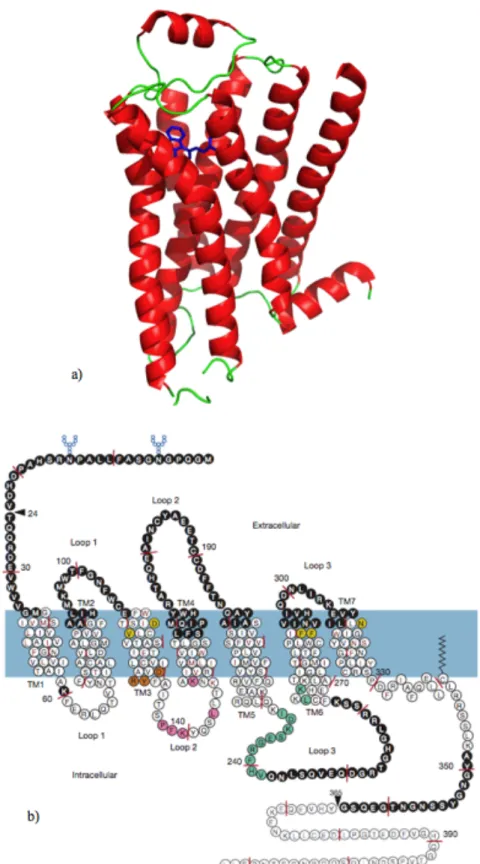
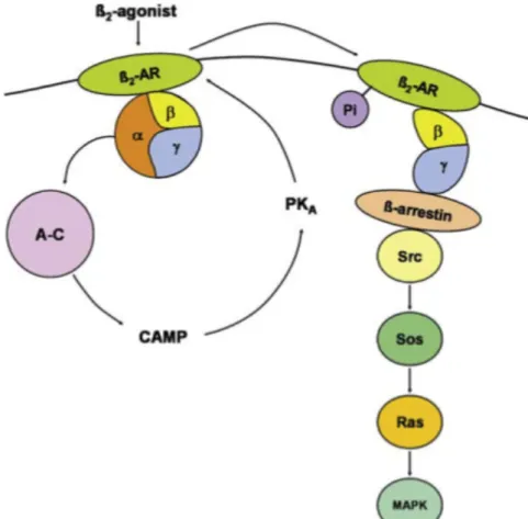
ß2AR has seven transmembrane (TM) domains, which is the main characteristics of the structure (Figure 2.1a). These seven TM domains are connected to each other with three extracellular loops and three intracellular loops. GPCRs are membrane-embedded proteins. Amino terminus is located in extracellular milieu and carboxyl terminus is located in cytosol (Figure 2.1b).

(19)

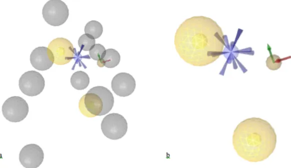
Figure 2.1. Shematic representation of GPCRs. (a) 3D modeling of ß2AR in cartoon representation. Red shows the 7TMs, greens are extracellular and intracellular loops and the inverse agonist Carazolol in blue with stick representation. The figure was prepared with Pymol.

(20)

2.2 Functional Role of Beta-2-Adrenergic Receptors

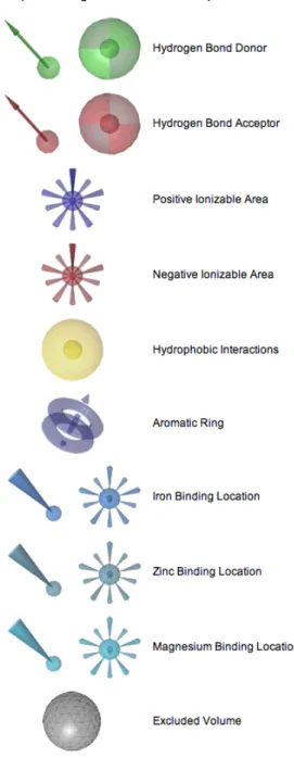
ß2ARs are responsible for signal transduction between the cell and the environment. They become active by hormones and neurotransmitters [20]. Figure 2.2 demonstrates the activation mechanism of ß2AR [21]. Upon activation of the receptor by a bound agonist diffusing from extracellular side, ß2AR interacts with a G protein nearby. G-protein consists of three subunits: α, β and γ. Followed by contact, guanosine diphosphate (GDP) inside the α-subunit is replaced by guanosine thriphosphate (GTP). The affinity of α-subunit is dramatically reduced for ß2AR, thus dissociates and couples with adenylate cyclase (A-C in Figure 2.2). Adenylyl cyclase causes an increase in cyclic adenosine monophosphate (cAMP) level, which catalyzes the activation of protein kinase A (PKA). PKA induces phosphorylation (Pi) of ß2AR and uncoupling of Gs. The phosphorylated ß2AR bound to β and γ subunits of G protein, couples to Gi proteins. β and γ subunits act as a scaffold for intracellular proteins such as ß-arrestin, Src, SOS and RAS, which leads to the activation of mitogen-activated protein kinase (MAPK) pathway.

ß2AR acts on smooth muscle relaxation, therefore its activation through agonists are used as treatment of asthma. It is believed that pKA phosphorylates key regulatory proteins involved in the control of muscle tone. In addition, cAMP decreases the Ca+2 level inside the cell, leading to muscle relaxation in the pulmonary airways. ß2AR also increases heart rate and cardiac muscle contractility with a minor degree compared to ß1AR. In addition, its stimulation increases pressure inside eye, therefore for glaucoma patients, its inhibition with an antagonist such as timolol, is required.

(21)

(22)

Chapter 3 Materials and Methods

3.1 Generating a Pharmacophore Model

The term pharmacophore was defined as, “the ensemble of steric and electronic features

that is necessary to ensure the optimal supramolecular interactions with a specific biological target structure and to trigger (or to block) its biological response” by

Wermunt et al. in 1968 [22]. Since then, it became a standard definition for pharmacophore concept accepted worldwide. Pharmacophores are not real molecules or they are not functional groups. They just represent the essential points of drug molecules for an optimal interaction with the target protein [23] and these interactions are Hydrogen-bonding, charge transfer, electrostatic and hydrophobic interactions. The pharmacophore model combined all these interaction in 3D space.

In modern drug discovery, there are two types of techniques, which help to design a drug: ligand-based drug design (LBDD) and structure-based drug design (SBDD). LBDD techniques rely on a set of drug molecules that are known to bind to a certain target with a known activity. The pharmacophore model consists of the chemical features shared by all known drug molecules. On the other hand, SBDD techniques rely on the knowledge of a three-dimensional structure of the protein [1] and the native state of the bound ligand. The pharmacophore model is composed of the interacting groups of the ligand with surrounding residues of the target protein.

(23)

With the increase in the amount of experimental data about the protein’s crystal strcutures, SBDD has become more powerful than LBDD [24]. Many popular software programs that generate pharmacophore models emerged and a few of them are Phase by Schrödinger [25], GASP (Genetic Algorithm Superposition Program) by Jones et al. and Catalyst by Accelrys [26] and finally LigandScout by inte:ligand [27], which was used in thesis.

LigandScout is using a structure-based approach to generate the pharmacophore model. It also provides a powerful visualization interface. It represents pharmacophore points by using special features, which are illustrated in Figure 3.1. These features determined based on two constraints: distance and direction. LigandScout selects two points. One point must be located on the protein while the other one must be located on ligand. It analyzes the relationship between these two points by distance constraints. Based on the information in LigandScout, default distance constrains are listed as in Table 3.1. On the other hand, to analyze the relationship between two atom groups instead of points, LigandScout uses direction constraints.

Table 3.1. LigandScout’s default distance constraints.

Aromatic interaction with positive ionizable 3.5 – 5.5 Å Aromatic interaction with ring (parallel) 2.8 – 4.5 Å Aromatic interaction with ring (orthogonal) 2.8 – 4.5 Å

H-Bond interaction 2.2 – 3.8 Å

Hydrophobic interaction 1.0 – 5.9 Å

Iron binding location 1.3 – 3.5 Å

Magnesium binding location 1.5 – 3.8 Å

Negative ionizable interaction 1.5 – 5.5 Å

Positive ionizable interaction with negative ionizable 1.5 – 5.5 Å

Positive ionizable with aromatic ring 1.0 – 10.0 Å

(24)

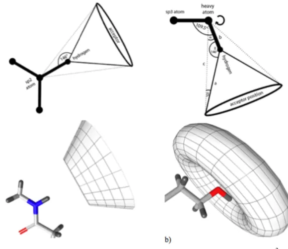
As shown in Figure 3.1, hydrogen bond features are represented by both distance and direction constraints while hydrophobic interactions and ionizable areas are shown with only a distance constraint. LigandScout can distinguish between flexible hydrogen bonds and rigid hydrogen bonds. Rigid hydrogen bond donors occur at sp2 hybridized heavy atoms and they illustrated by a cone with cutoff apex (Figure 3.2.a). Flexible hydrogen bond donors occur at sp3 hybridized heavy atoms and they are illustrated by a torus (Figure 3.2.b). For a valid hydrogen bond, the angle between Hydrogen-bond atom vector and hydrogen vector must be below the defined constraints (default: 50.00o for rigid H-bond, 34.00o_{for flexible H-bond). To define a hydrogen bond acceptor,} LigandScout takes neighboring atoms in considerations and calculates the weighted vector. This vector’s angle must be below the defined constraint (default: 85.00o_).

Hydrophobic features are depicted with distance constraints. There are two thresholds that change the effect of hyrophobicity: minimum threshold and surface accessibility threshold. Minimum threshold analyzes the hydrophobic moiety and determines the minimum hydrophobic threshold of groups, rings and chains. Less hydrophobic regions can be determined when the minimum threshold value is increased. Surface accessibility threshold determines the sterical accessibility due to the hydrophobic moiety. Increasing the surface accessibility threshold causes more restrict identification.

LigandScout defines aromatic features according to the interaction of the ligand and it’s environment. Orthogonal, parallel (π-π) and cation-π interactions are considered to determine the aromatic region. To determine excluded volumes, LigandScout determines the shape of the active site and the conformation of the protein. Excluded volumes increase the selectivity of the pharmacophore model.

(25)

LigandScout also provides two different alignment options to its users when dealing with more than one pharmacophore model: a “shared” pharmacophore model consists of the pharmacophore features shared by all models, whereas the “merged” pharmacophore combines all pharmacophore features encountered in any model.

Figure 3.1. Pharmacophore representation in LigandScout. Picture taken from inteligand website.

(26)

Figure 3.2. Hydrogen bond constraints. (a) Rigid H-bonds constraint of an sp2 hybridized amide nitrogen. (b) Flexible hydrogen bonding constraint of an sp3 hybridized hydorxy group. Pictures are taken from manual of LigandScout.

3.2 Virtual Screening

Discovering a new drug is a long term and expensive process. To make this process faster and cheaper, molecules that do not have the desired activities must be eliminated in early stages. For that purpose, screening methodologies have been developed. Ligands with desired activities can be identified experimentally, by high-throughput screening (HTS) of databases including millions of compounds. However, this is a time-consuming and expensive process. Therefore, as an alternative to HTS, virtual screening (VS) became a useful tool for drug discovery [28]. The aim of VS is to determine proper molecules with required properties by screening massive chemical databases in a short period of time at low costs [29]. Generally, VS techniques can be divide into two

(27)

groups: Pharmacophore-based virtual screening and Docking-based virtual screening, which are described in detail in the following two sections.

3.2.1 Pharmacophore-based Virtual Screening (PBVS)

Pharmacophore-based screening is useful when the three-dimensional structure of the target protein is not known. Moreover, if 3D structure of a target is known, both docking-based and pharmacophore-based virtual screening methods can be used [30]. A screened molecule is counted as a hit if it contains the required pharmacophore features of the proposed model. Pharmacophore-based screenings are around ten thousand times faster than docking-based screenings, thus they are usually preferred over docking as an initial filter to remove the molecules which do not have essential features for binding [31]. Docking can be used in later stages for a more detailed evaluation of the hit compounds.

In this thesis, the ZINC database was screened using a pharmacophore-based virtual screening tool provided by LigandScout. The program accepts the proprietary LDB file format for molecule libraries. More than one database can be screened simultaneously against the selected pharmacophore. Also, it provides the users to mark their databases as active or inactive to the activity of molecules in the database. In addition, users can customize several screening settings [29]. For instance, LignadScout has two types of scoring functions options. One of them is Pharmacophpre-Fit (PF) scoring function. It considers just pharmacophoric features and their RMSD values. The other one is Relative Pharmacophore Fit (RPF) scoring function. RPF scores the amount of the matching pharmacophoric features and normalized the aligned pharmacophores to [0..1]. Moreover, maximum number of features that can be omitted during the screening process, can be specified. If maximum number of omitted features is defined as zero than all pharmacophoric features should be matched to be a valid hit. Check exclusion volume option enables the consideration of exclusion volumes during the screening process.

(28)

3.2.2 Docking-based Virtual Screening (DBVS)

Nowadays, docking-based virtual screening techniques are widely used in drug discovery and many important drugs on the market are discovered in silico [29]. DBVS generates all possible poses of the small molecule to find out the nest configuration to from a protein-ligand complex [32]. Hence, two characteristics of the docking tool are critical: configuration search algorithm and scoring function (SF). The search algorithm predicts all possible binding modes of the ligand in the receptor’s binding pocket. SF ranks them according to the score vale and accepts the conformation with the highest score as the most plausible binding mode [33]. At the end of screening, all docked ligand molecules are sorted based on their score values, and the ligand molecules at the top of the list are selected as hit molecules. The top of the list can be defined either as a small percentage of the whole database or using a threshold score value.

3.3 Docking methodology and Scoring Functions

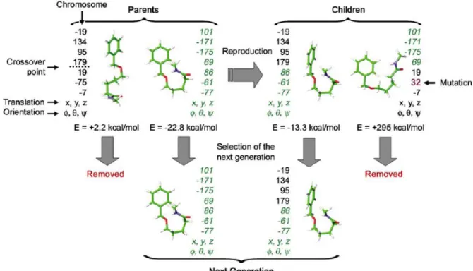
Currently, many software tools exist for docking. Every tool has its own pose generation methods and scoring functions [28]. Both AutoDock and GOLD software tool used in thesis, use genetic algorithm to search the conformational score. In genetic algorithm, the ligand is represented by a set of torsion angles of rotatable bonds resembling to the set of genes in a chromosome. As shown in Figure 3.3, genetic algorithm starts by creation of a population, composed of randomly generated ligand conformations, the so-called “parents” [33]. Then, these parent conformations reproduce new conformations by transmitting genetic information between each other by crossover and mutation, e.g. by exchanging randomly their torsion angles as shown in Figure 3.3. As a result, children ligand poses are generated. Next, the energies of these new conformations were evaluated. The ones with the lowest energies (or highest scores) were selected as members of the next generation. This iteration continues until the best conformation with the highest score is obtained.

(29)

Figure 3.3 Schematic representation of the genetic algorithm.

Soring functions are the important part of a docking tool because the binding poses that are generated from DBVS must be evaluated to recognize the correct pose which would resemble the native binding conformation. There are three principles of scoring [28]: (i) to recognize native binding mode, (ii) to estimate binding affinities correctly, and (iii) to recognize active compounds from poor binders. Current SF’s are divided into three groups as force-field based (FF), empirical and knowledge-based [34].

Force-field scoring functions are based on different force field parameter sets, such as CHARMM [35] and AMBER [36]. The interaction between a ligand and a receptor is most often described by sum of van der Waals (VDW), hydrogen bond and electrostatic terms, which are defined with 12-6 Lennard-Jones potential, 12-10 Lennard-Jones potential and Coulombic formulation, respectively. For example, AutoDock is based on the AMBER force field [37] as given in equation 1.

(30)

∆𝐺 = ∆𝐺_!"# ( !!" !_!"!" !,! −!_!!" !"! ) + ∆𝐺_ℎ!"#$ 𝐸 𝑡 !!" !_!"!"− !!" !_!"!"+ 𝐸ℎ!"#$ + !,! ∆𝐺!"!# _{! !}!!!! !" !!"+ ∆𝐺!"#𝑁!"#+ !,! ∆𝐺_!"# 𝑆_!𝑉_!𝑒(!!!" ! !!!) !,!

The first term of this equation is the 12-6 Lennard-Jones potential. rij is the distance between protein atom i and ligand atom j, Aij and Bij are the VDW parameters. The second term is the 12-10 Lennard-Jones potential. E(t) function provides directionality based on the angle t from ideal hydrogen bonding geometry. The third term is the Coulomb formulation for electrostatics. ε(rij) stands for distance-dependent dielectric

constant, qi and qj are the atomic charges. Final term is a desolvation potential. V stands for the volume of the atoms and S represents the solvation parameter.

GoldScore is also a force-field based scoring function and consists of four components namely, protein-ligand hydrogen bond energy and van der Waals energy, ligand internal van der Waals energy and ligand torsional energy. GoldScore scoring function is defined as:

ƒ = 𝑆_{ℎ!_!"#}+ 𝑆_{!"#_!"#}+ 𝑆_{ℎ!_!"#}+ 𝑆_{!"#_!"#}

where, Shb_ext is the protein-ligand hydrogen bonding score, and Shb_int is the internal hydrogen bonding of the ligand. SVDW_ext and SVDW_int are the van der Waals scores.

Empirical scoring functions are derived using the experimentally determined binding affinities and structural information. They are the sum of uncorrelated terms with coefficients obtained from regression analysis. X-Score, GlideScore and ChemScore are the examples. ChemScore scoring function defined as [38]:

(3.1)

(31)

∆𝐺_!"#$"#% = ∆𝐺_!+ ∆𝐺_ℎ!"#$+ ∆𝐺_!"#$%+ ∆𝐺_!"#$ + ∆𝐺_!"#

Each component of this equation is the product of a term dependent on the magnitude of a particular physical contribution to free energy and regression coefficients. According to this information, those components can be written as:

∆𝐺_!"#$"#%= 𝑣_!+ 𝑣_!𝑃_ℎ!"#$+ 𝑣_!𝑃_!"#$%+ 𝑣_!𝑃_!"#$ + 𝑣_!𝑃_!"#

where, v terms represent regression coefficients and P terms are various types of physical contributions to binding.

ChemScore value is obtained by adding in a clash penalty and internal torsion terms. Covalent and constraint scores may also be added.

𝐶ℎ𝑒𝑚𝑆𝑐𝑜𝑟𝑒 = ∆𝐺!"#$"#%+ 𝑃!"#$ℎ+ 𝑐!"#$%"&'𝑃!"#$%"&'+ (𝑐!"#$%&'(𝑃!"#$%$&'(

+ 𝑃_!"#$%&'(#%)

Knowledge-based scoring functions’s parameters are derived from experimentally determined X-ray structures of protein-ligand complexes. They are calculated using Boltzmann distribution law, as:

𝑤 𝑟 = −𝑘_!𝑇𝑙𝑛[𝜌 𝑟 𝜌∗ _𝑟 ]

where w(r) represents the all potential parameters, kB is the Boltzmann constant, T is the absolute temperature of the system, ρ(r) is the number density of the protein-ligand atom pair at distance r in the training set and ρ*_{(r) is the pair density in a reference state where} the interatomic interaction are zero. DrugScore and GOLD/ASP are examples of knowledge-based SFs [33,39].

(3.4)

(3.5)

(32)

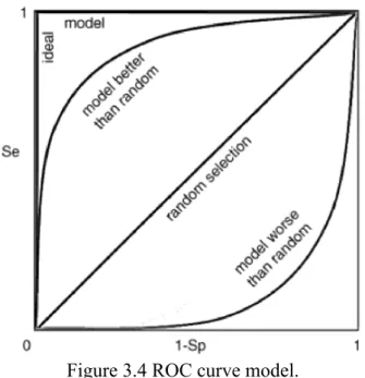
3.4 Receiver Operating Characteristic (ROC) Curve

Pharmacophore-based virtual screening (PBVS) is a widely used method in drug discovery. A pharmacophore model that is generated for PBVS should be able to enrich as many active compounds as possible for selected database. There are several methods that ensure this enrichment. Receiver Operating Characteristic (ROC) curve is one of these methods [29]. ROC curves can be easily analyzed visually. It is used for selecting appropriate threshold values, which gives the maximum ratio of active molecules to inactive molecules. [40]. ROC curve graph is derived from sensitivity (Se) value on the

y-axis and 1-specificity (Sp) value on the x-axis. Se is the ratio of the number of selected

active molecules and the number of all active molecules in the database. In other words,

Se gives the rate of true positives and is calculated as [29]:

𝑆𝑒 =𝑆𝑒𝑙𝑒𝑐𝑡𝑒𝑑 𝑎𝑐𝑡𝑖𝑣𝑒𝑠 𝐴𝑙𝑙 𝑎𝑐𝑡𝑖𝑣𝑒𝑠 =

𝑇𝑃 𝑇𝑃 + 𝐹𝑁

where TP is true positives, FN is false negatives. Sp is the ratio of inactive molecules not selected by the model and all inactive molecules in the database. It defines the capability of pharmacophore model to eliminate inactive molecules. Sp is defined as [29]:

𝑆𝑝 = 𝐷𝑖𝑠𝑐𝑎𝑟𝑑𝑒𝑑 𝑖𝑛𝑎𝑐𝑡𝑖𝑣𝑒𝑠 𝐴𝑙𝑙 𝑖𝑛𝑎𝑐𝑡𝑖𝑣𝑒𝑠 =

𝑇𝑁 𝑇𝑁 + 𝐹𝑃

where TN is true negatives, FP is false positives. Accordingly, 1-Sp becomes [29]:

1 − 𝑆𝑝 = 𝐹𝑃 𝑇𝑁 + 𝐹𝑃

ROC curve represents all possible Se and 1-Sp values of a molecule obtained from PBVS, using different thresholds, such as a scoring function defining the goodness of a hit molecule. ROC curve starts from the origin. The diagonal line represents the case where the pharmacophore model cannot make a distinction and molecules are selected

(3.7)

(3.8)

(33)

randomly. If ROC curve is located above the diagonal line, it represents a pharmacophore model that enriches more active compounds than inactive compounds. If the ROC curve is below the diagonal line, it indicates simply that the pharmacophore model’s ability to distinguish actives from inactives is worse than random (Figure 3.4) [29].

Figure 3.4 ROC curve model.

3.5 ZINC Database

Since structure-based drug design has become a powerful technique for drug discovery, the need for suitable databases has increased. These databases have to be easily accessible and they must be comprised of proper data. Lots of databases were generated to supply these needs, such as ChemNavigator [41], Ligand.Info [42], The ChemBank project [43]. However, these databases do not meet the exact requirements. For instance, the ChemBank contains only 2D molecules. Availability of 3D structures of each molecule that are going to be screened is very important for structure based virtual screening [16].

(34)

In 2005, John Irwin and Brain Shoichet introduces ZINC database [16], which includes 3D structure of each molecule. Also, some physical properties such as molecular weight, predicted logP, number of hydrogen bond donors, number of hydrogen acceptors, number of rotatable bonds, net charge, number of rigid fragments, number of chiral centers, number of chiral double bonds and a polar desolvation energy value. ZINC is a freely accessible database. Multiple file formats are available such as SMILE, mol2, 3D SDF and DOCK feasible format. Users can download the entire ZINC database or they can download a set of molecules that satisfy certain physical properties listed above, based on user’s research interest. Moreover, they can upload their own molecules to ZINC database as well.

3.6 Rescoring

Docking programs generate a score value for every pose according to their scoring functions and rank them accordingly. Yet, these scores may not be strong enough to make good predictions in all cases. This is the main reason for the use of rescoring functions. These functions simply rescore all the poses obtained from a docking program and reevaluated them. These scoring functions try to enhance predictive power of docking tools [44]. In this thesis, DSX (Drug Score eXtended), which is a knowledge-based scoring function, is used for rescoring the poses obtained from AutoDock. The pair potentials are derived from protein-ligand complexes as stored in the PDB DataBank.

(35)

Chapter 4 Results and Discussions

4.1 Generation of the Pharmacophore model

Five crystal structures of ß2-AR in the inactive state were used for the generation of a pharmacophore model via LigandScout software tool [27]. Their PDB entries are 2RH1 (inverse agonist: carazolol), 3D4S (inverse agonist: timolol), 3NY8 (inverse agonist: ICI118,551), 3NY9 (inverse agonist: JSZ), and 3NYA (antagonist: Alprenolol). LigandScout determines the pharmacophoric features according to some distance constraints between the macromolecule and its ligand. These constraints were listed in Table 3.1 in previous chapter.

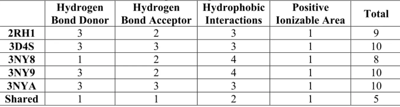
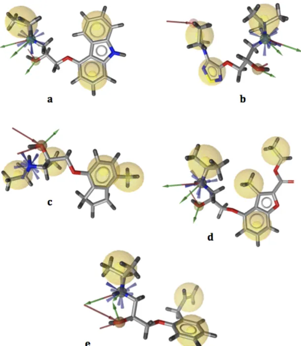
First, a pharmacophore model was created for each complex structure as shown in Figure 4.1, and listed in Table 4.1. 2RH1 has a total of nine pharmacophoric features: three hydrogen bond (H-bond) donors, two H-bond acceptors, three hydrophobic regions, and one positive ionizable area (Figure 4.1a). 3D4S consists of three H-bond donors, three H-bond acceptors, three hydrophobic areas, and one positive ionizable area (Figure 4.1b). 3NY8 includes one H-bond donor, two H-bond acceptors, four hydrophobic interactions, and one positive ionizable area (Figure 4.1c). 3NY9 has three H-bond donors, two H-bond acceptors, four hydrophobic interactions, and one positive ionizable area (Figure 4.1d). 3NYA consists of ten pharmacophoric regions: three H-bond donors, three H-H-bond acceptors, three hydrophobic interactions and one positive ionizable area (Figure 4.1e).

(36)

Next, a shared pharmacophore model was obtained after aligning all five models via LigandScout. The shared pharmacophore model consists of five pharmacophoric features that are common to all five pharmacophore models (Figure 4.2). As listed in Table 4.1, these features include one H-bond donor, one H-bond acceptor, two hydrophobic interactions, and one positive ionizable area. Figure 4.2 shows the model with and without excluded volumes.

Table 4.1 Number of pharmacophore features in five inactive crystal structures and the shared pharmacophore model.

Hydrogen Bond Donor Hydrogen Bond Acceptor Hydrophobic Interactions Positive

Ionizable Area Total

2RH1 3 2 3 1 9 3D4S 3 3 3 1 10 3NY8 1 2 4 1 8 3NY9 3 2 4 1 10 3NYA 3 3 3 1 10 Shared 1 1 2 1 5

(37)

Figure 4.1 Pharmacophore models of five X-ray crystal structures of human-ß2AR with PDB ids (a) 2RH1, (b) 3D4S, (c) 3NY8, (d) 3NY9, (e) 3NYA (a-e). Pharmacophore models generated via LigandScout. Yellow and blue spheres represent hydrophobic areas, and positive ionizable areas, respectively. Green and

(38)

Figure 4.2. Pharmacophore features of the shared pharmacophore model (a) with and (b) without excluded volume. See the caption of Figure 4.1 for more explanation

about illustration.

4.2 ZINC Database

ZINC Database includes 19,607,982 purchasable molecules as of January 2013. According to some physical properties, these molecules were categorized into three subsets: Lead-Like, Fragment-Like and Drug-Like. The Lead-like subset includes molecules with molecular weight between 250 and 350 daltons, logP value less than or equal to 3.5, and the number of rotatable bonds less than or equal to 7. The Fragment-Like subset consists of molecules having molecular weight 250 or less, calculated logP less than or equal to 3.5 and number of rotatable bonds less than or equal to 5. The Clean Drug-Like subset, selected for screening process of our study in this thesis, consists of 9,928,465 molecules and complies with the Lipinski’s Rule of five. In addition, other desirable physical properties for drug likeliness such as partition coefficient (xlogP) and number of rotatable bonds are also observed in these molecules, as listed in Table 4.2.

(39)

Table 4.2. Physical Properties of Clean Drug-Like subset of ZINC Database.

Molecular Weight (g/mol) 150 ≤ mwt ≤ 500

xlogP xlogP ≤ 5

Number of Rotatable Bonds Rb ≤ 7

Polar Surface Area (Å2) tPSA < 150

Number of H-bond Donors Hbd ≤ 5

Number of H-bond Acceptors Hba ≤ 10

4.3 Set of Compounds with Known Activities

A decoy set was created to validate the reliability of the shared pharmacophore model using GLIDA GPCR-Ligand Database [45]. There exist many databases related to GPCRs, such as GPCRDB [46], IUPHAR [47], which comprise data about biological aspects of proteins [17]. However, GLIDA is different from other databases, in the fact that it includes novel and GPCR oriented molecules. It focuses on the importance of ligands as drug leads. GLIDA provides three kinds of data: biological information about GPCRs, the chemical information about their ligands, and, the binding information of specific GPCR ligands. All that data about these GPCRs was obtained from three species: human, rat and mouse since these species have an effective role in drug discovery process. In addition, GLIDA provides a user-friendly interface [48], over which users can search a molecule according to a ligand or a GPCR protein. It demonstrates the ligand structures and lists the correlation maps that show the relation between the structure of the protein and the property of the ligand. Moreover, users can acquire information on the activity types of the ligand.

GLIDA provides a total 317 agonists and 259 antagonists for human ß2-adrenergic receptor. During the creation of our decoy set, the structural diversity was taken into account. Thus, compounds that have similar structures were eliminated. The final decoy set consisted of a total 117 distinct molecules of which 53 were antagonists and of which 64 were agonists. Corina [49] program was used to transform these molecules into 3D mol2 format. These molecules were depicted in Appendix A and Appendix B.

(40)

4.4 Pharmacophore-Based Screening of the decoy set and the Clean Drug-Like Subset of ZINC Database

In order to validate how well the shared pharmacophore model discriminates the antagonists from agonists or non-inhibitors, the decoy set was first screened using the shared pharmacophore model using LigandScout software tool. LigandScout presents two different scoring functions: Pharmacophore Fit and Relative Pharmacophore Fit. Furthermore, the maximum number of omitted features, which signifies the maximum number of query features that can be left out during screening can be adjusted. Finally, the exclusion volume can be left checked or unchecked. Exclusion volume represents the sterically occupied regions by the receptor. All of these variables affect the result of a virtual screening. To determine an optimum solution, several runs have been applied to the decoy set using various combinations of these variables.

Initially, a screening was performed using the default values that are given at the third entry of Table 4.3 (Scoring function = Relative Pharmacophore Fit, Maximum Number of Omitted Features = 2, Check exclusion volume = On). Accordingly, molecules were counted as hits, if they had at least three pharmacophoric features out of five and if they fit properly in the area that was defined by exclusion volumes. As a result of this screening, 82 hits were found. 45 of them were antagonists (active), and 37 of them were agonists (inactive). After that, screening was repeated three times using maximum number of omitted features as 0,1, and 3 and the results were listed in Table 4.3. As expected, increasing the number of omitted features increased the number of hits as well, since less number of pharmacophoric features are required to become a hit. On the other hand, the number of false positives (agonists) has increased as well. ROC (Receiver Operating Characteristic) curves for each screening were determined using LigandScout and illustrated in Figure 4.3.

(41)

Table 4.3 Screening results using different values for the maximum number of omitted features.

RUN # _FunctionScoring

Max. Number of Omitted Features Check Exclusion Volumes Number of Antagonists/ Total Antagonists1 Number of Agonists / Total Agonists2 Total Hits / Total Compounds3 1 RPF4 0 On 19 / 53 1 / 64 20 / 117 2 RPF 1 On 37 / 53 12 / 64 49 / 117 3 RPF 2 On 45 / 53 37 / 64 82 / 117 4 RPF 3 On 45 / 53 38 / 64 83 / 117 5 PF5 0 On 19 / 53 1 / 64 20 / 117 6 PF 1 On 37 / 53 12 / 64 49 / 117 7 PF 2 On 45 / 53 37 / 64 82 / 117 8 PF 3 On 45 / 53 38 / 64 83 / 117

1_{Total number of antagonists in the decoy set was 53.} 2 _{Total number of agonists in the decoy set was 64.} 3_{Total compounds in the decoy set was 117.} 4 _{Relative Pharmacophore Fit}

5_{Pharmacophore Fit}

Next, the scoring function was changed to Pharmacophore Fit to see the effect on the screening results. Check exclusion volume option was “on” during this run as well. The number of omitted features option was changed similarly. Results were listed in Table 4.3. Same results were obtained with the same ROC curves, which means the scoring function did not have any effect on the screening.

Next, screenings were performed to understand the effect of exclusion volumes. Check exclusion volumes option was set to “off”. First, Relative Pharmacophore fit scoring function was chosen and the maximum omitted features were increased from zero to three (Table 4.4). Then, the scoring function was changed to Pharmacophore Fit scoring and the number of omitted features was changed. Similar to previous results, the scoring function had no effect on the results. However, the number of hits changed with the maximum number of omitted features, as seen previously with excluded volumes. The corresponding ROC curves are illustrated in Figure 4.4 for run numbers 9 through 12.

(42)

Figure 4.3 ROC curves of the screening results using different values for the maximum number of omitted features. (a) RUN#1. AUC1,5,10,100%: 1.00; 1.00; 1.00; 0.67 and EF1,5,10,100%: 2.2; 2.2; 2.2; 2.1. (b) RUN#2. AUC1,5,10,100%: 1.00; 1.00; 1.00; 0.81 and EF1,5,10,100%: 2.2; 2.2; 2.2; 1.7. (c) RUN#3. AUC1,5,10,100%: 1.00; 1.00; 1.00; 0.83 and EF1,5,10,100%: 2.2; 2.2; 2.2; 1.2. (d) RUN#4. AUC1,5,10,100%: 1.00; 1.00; 1.00;

(43)

Table 4.4 Screening results when check exclusion volumes option was “off”. RUN # Scoring Function Max. Number of Omitted Features Check Exclusion Volumes Number of Antagonists/ Total Antagonists1 Number of Agonists / Total Agonists2 Total Hits / Total Compounds3 9 RPF4 ₀ _Off _{24 /53} _{3 / 64} _{27 / 117} 10 RPF 1 Off 47 / 53 39 / 64 86 / 117 11 RPF 2 Off 51 / 53 63 / 64 114 / 117 12 RPF 3 Off 51 / 53 63 / 64 114 / 117 13 PF5 ₀ _Off _{24 / 53} _{3 / 64} _{27 / 117} 14 PF 1 Off 47 / 53 39 / 64 86 / 117 15 PF 2 Off 51 / 53 63 / 64 114 / 117 16 PF 3 Off 51 / 53 63 / 64 114 / 117

1 _{Total number of antagonists in the decoy set was 53.} 2 _{Total number of agonists in the decoy set was 64.} 3_{Total compounds in the decoy set was 117.} 4 _{Relative Pharmacophore Fit}

As expected, more hits were obtained when check exclusion volumes option was off. However, the number of agonists (false positives) as hit molecules, has increased as well. Accordingly, more accurate hits were acquired when check exclusion volumes option was on.

LigandScout allows the user to select any excluded volume and discard it. To increase the discriminatory power of the pharmacophore model, two outmost excluded volumes were deleted as shown in Figure 4.5. New screenings were performed with Relative Pharmacophore Fit scoring function and this new “modified” model (Table 4.5). The main goal of this trial was to obtain more active molecules (antagonist) than inactive ones (agonists).

(44)

Figure 4.4 ROC curves of the screening results when check exclusion volume option was “off”. (a) RUN#9. AUC1,5,10,100%: 1.00; 1.00; 1.00; 0.71 and EF1,5,10,100%: 2.2; 2.2; 2.2; 2.0. (b) RUN#10. AUC1,5,10,100%: 1.00; 1.00; 1.00; 0.81 and EF1,5,10,100%: 2.2; 2.2; 2.2; 1.2. (c) RUN#11. AUC1,5,10,100%: 1.00; 1.00; 1.00; 0.80 and EF1,5,10,100%: 2.2;

2.2; 2.2; 1.0. (d) RUN#12. AUC1,5,10,100%: 1.00; 1.00; 1.00; 0.80 and EF1,5,10,100%: 2.2; 2.2; 2.2; 1.0.

(45)

Figure 4.5 Two exclusion volumes, which were circled in red color, were deleted. Picture was taken from LigandScout.

Table 4.5 Screening results of “modified” pharmacophore model using different values for the maximum number of omitted features.

RUN # Scoring Function Max. Number of Omitted Features Check Exclusion Volumes Number of Antagonists/ Total Antagonists1 Number of Agonists / Total Agonists2 Total Hits / Total Compounds3 1 RPF4 ₀ _On _{19 / 53} _{1 / 64} _{20 / 117} 2 RPF 1 On 37 / 53 12 / 64 49 / 117 3 RPF 2 On 45 / 53 37 / 64 82 / 117 4 RPF 3 On 46 / 53 38 / 64 83 / 117

1 _{Total number of antagonists in the decoy set was 53.} 2 _{Total number of agonists in the decoy set was 64.} 3_{Total compounds in the decoy set was 117.} 4 _{Relative Pharmacophore Fit}

According to the results in Table 4.5, deleting two exclusion volumes did not affect the screening process. Equal number of hits was obtained from both original pharmacophore model and the modified one. After careful evaluations of ROC curves, ROC curves with the highest AUC (Area Under the ROC Curve) values of 0.83 were obtained using the Relative Pharmacophore Fit score when check exclusion volume option was on and the maximum number of omitted features was either 2 or 3 (RUN#3 and #4 in Table 4.3). As the third run provides less inactive compounds (37 agonists) than the fourth run (38 agonists) with the same number of active compounds (45 antagonists), the set of parameters in RUN #3 (Relative

(46)

volume: on) has been selected for further screening of the ZINC database. They were also the default parameters of LigandScout software tool.

Prior to screening ZINC database, a threshold value, which corresponds to a so-called “model exhaustion” or “cut-off” point on the selected model’s ROC curve, must be specified. Hit molecules that have a Relative Pharmacophore Fit score value less than this threshold will be eliminated. This value is determined from the point on the ROC curve where there exists a considerable amount of true positives (antagonists) with respect to false positives (agonists) among the hit molecules. As shown in Figure 4.6 the exhaustion point (red dot on the curve) was determined as (0.27,0.83), which represents the percentage of true positives as 83 (44 antagonists) and the ratio of false positives as 27 (17 agonists). The lowest score value of these 61 (44 + 17) molecules was determined as 0.64, which was taken as the threshold value for the screening of ZINC database.

Using the shared pharmacophore model with default parameters of LigandScout mentioned above a total of 9.928.495 molecules of the Clean Drug-Like subset of ZINC was screened and hit molecules were eliminated if their Relative Pharmacophore Fit score value was under 0.64. Finally, a total of 729.413 molecules with a score value above 0.64 remained and was further evaluated with several docking experiments, alongside the decoy set of 61 molecules. These results are discussed in the next part

(47)

Figure 4.6 ROC Curve for Run #1. Red dot illustrates the model exhaustion point, which corresponds to 83% true positives and 27% false positives.

4.5 Docking and Binding Evaluations

To further evaluate the hit molecules, 61 molecules (44 antagonists and 17 agonists) from decoy set and 729.413 compounds from clean drug-like subset of ZINC database were docked to the inactive crystal structure (PDB id: 2RH1) using GOLD and AutoDock software tools. The crystal structure with PDB id 2RH1 was selected due to its high resolution, which is 2.40

Å.

On the other hand, resolutions of structures with PDB ids 3D4S, 3NY8, 3NY9 and 3NYA are reported as 2.80 Å, 2.84 Å, 2.84 Å, and 3.16 Å, respectively.

The first docking was performed using GOLD with CHEMPLP scoring function. Default features were used (radius: 10 Å, ga run: 10, ga search: SLOW). The docked poses with the highest scores were analyzed based on some key residues for

(48)

includes Ser203, Ser204 and Ser207 while second group consists of Asp113, Val114 and Asn312. According to the binding test, the docked pose of each compound with the highest score has to be interacting with at least one residue from each group. Otherwise, it is eliminated. A total of 58 molecules (41 antagonists and 17 agonists) from the decoy set have passed the binding test (designed as binding test #1 in Figure 4.8). On the other hand, 610.490 compounds out of 729.413 compounds from ZINC database have passed the binding test. Next, a threshold of 85 for ChemPLP score value was selected for further elimination. 23.568 ZINC compounds, 17 antagonists and 3 agonists have been selected as they had score values above 85. These results correspond to an enrichment factor of 11.9 for 3.2% database coverage calculated using the equation below:

𝐸𝑅 = !"

!

(_!!)

where TP is the number of true positives (antagonists), which is 17, n is the total number of compounds with a score value above 85 and is equal to 23.588 (=23.568 ZINC compounds + 17 antagonists + 3 agonists), A is the number of active compounds (antagonists) which is 44, and N is the total number of compounds screened which is 729.474 (=729.413 + 44 antagonists + 17 agonists). 3.2% simply corresponds to the n/N x 100.

(49)

Figure 4.7 Extracellular view of key residues for binding test #1. Blue illustrates the first group (Ser204, Ser203 and Ser 207). Red illustrates the second group (Asn312,

Asp113 and Val114). Pink illustrates the partial inverse agonist Carazolol. The selected 23.568 molecules were redocked to the inactive crystal structure (PDB id: 2RH1) with AutoDock and GOLD. For every molecule, a total of 20 poses were generated from AutoDock and rescored with DSX scoring function. The best pose (with the highest score) was further evaluated based on its binding mode (designed as binding test #2 in Figure 4.8). In addition, each molecule was docked with GOLD using GoldScore and ChemScore as the scoring function. Similarly, the best pose of every molecule from each docking run was further evaluated based on its interacting residues (binding test #2). According to the second binding test, the most essential key residues for antagonist binding were determined and divided into two groups: Ser203, Asp113, Asn312, Tyr316 were found in the first group while Tyr286 and Asn293 formed the second group (Figure 4.9). Molecules have to interact with all the residues from first group and with at least one of the residues from the second group in order to pass the binding test #2. Otherwise, they were eliminated.

(50)

Figure 4.8 Flowchart of the screening process of the Clean Drug-Like ZINC database and the decoy set.

ZINC [Clean Drug Like Subset] 9,928,465 Compounds

DECOY SET [117 Molecules] 53 antagonists + 64 agonists Pharmacophore Screening Fit Value > 0.64 Docking with Autodock (DSX SCORE) & Binding test2 Docking with GoldScore & Binding test2 Docking with ChemScore & Binding test2

DSX Score > 150 GoldScore > 77 ChemScore > 42 DSX Score > 150 GoldScore > 77 ChemScore > 42

Merging all three sets Merging all three sets

Docking with Autodock (DSX SCORE) & Binding test2 Docking with GoldScore & Binding test2 Docking with ChemScore & Binding test2

Docking with GOLD (CHEMPLP) Binding Test1_{and Score > 85}

ADMET Filtering 729,413 compounds 61 molecules 44 antagonists + 17 agonists 23,568 compounds 20 molecules 17 antagonists + 3 agonists 360 compounds 3 antagonists 0 agonist 62 compounds 1 antagonist 9,712

compounds compounds 11,313 compounds 9,942 12 antagonists 1 agonist 11 antagonists 3 agonists 13 antagonists 2 agonists 7 antagonists 2 agonists 9 antagonists 1 agonist 8 antagonists 0 agonist 3,262 compounds 2,686 compounds 3,886 compounds

(51)

Figure 4.9 Extracellular view of key residues for binding test #2. Red represents the first group, blue represents the second group, and pink represents the partial inverse

agonist Carazolol.

Based on these criteria, docking all 23.588 molecules with AutoDock and rescoring with DSX yielded 13 molecules (12 antagonists, 1 agonist) from decoy set and 9.712 compounds from ZINC database that have passed the binding test #2. Similarly, docking with GOLD using GoldScore led to 11 antagonists and 3 agonists from decoy set and 11.313 compounds while docking with GOLD using Chemscore led to 13 antagonists and 2 agonists from decoy set and 9.942 compounds from ZINC database.

For further elimination, threshold values were determined for each scoring function used previously. Among those that have passed the binding test #2, molecules that have a score value above the threshold values have been selected for the next evaluation step. The threshold values were set to 150, 77 and 42 for DSX, GoldScore and ChemScore, respectively. Based on these threshold values, 8 antagonists from decoy set and 3.886 compounds from ZINC database had a DSX score value above 150. On the other hand, 9 antagonists and 1 agonist from decoy set and 2.686

(52)

finally, 7 antagonists and 2 agonists from decoy set and 3.262 compound from ZINC have been selected as they had a ChemScore over 42.

All these selected molecules were simply merged and a molecule was counted as a hit if it was found in all three groups, i.e., if it satisfied all the three threshold values. Consequently, 360 compounds from ZINC and 3 antagonist molecules from the decoy set satisfied the threshold values and were further evaluated based on their ADMET (Absorption, Distribution, Metabolism, Extraction and Toxicity) properties, using Discovery Studio tool by Accelrys [50].

4.6 ADMET Filtering

ADMET (Absorption, Distribution, Metabolism, Elimination, Toxicity) analysis is a crucial step in drug design. Molecules cannot be counted as drug candidates if they do not fulfill the requirement of ADMET properties. In this thesis, Discovery Studio tool from Accelrys was used for ADMET predictions. ADMET module of Discovery Studio makes predictions based solely on the chemical structure of the molecule. Human intestinal absorption (HIA) and blood brain barrier penetration are the two properties estimated by the program and used for our filtering.

3 antagonist molecules from decoy set and 360 compounds from ZINC database were analyzed based on these features. Figure 4.10 and 4.11 depicts the plot of polar surface area (ADMET_PSA_2D) versus the partition coefficient between n-octanol and water (ADMET _AlogP98) for 3 antagonists from the decoy set and 360 compounds from ZINC, respectively. Since Carvedilol (compound #1, antagonist from the decoy set) falls within all four ellipses in Figure 4.10, it fully satisfies the requirements of intestinal absorption and blood brain penetration. On the other hand, L023760 (compound #2) and L004107 (compound #3) do not fall into any ellipses, thus they were eliminated automatically. At the end of the ADMET filtering of decoy set, only one molecule was remained.

(53)

Figure 4.10 ADMET Plot of the decoy set. Carvedilol. L023760 and L004107 are represented with numbers 1, 2, and 3, respectively.

Figure 4.11 shows the ADMET plot of 360 molecules from ZINC database. All 360 molecules satisfied at least one of the required conditions that are blood brain penetration and intestinal absorption, but 62 of them were found inside all four ellipses, thus satisfied all two requirements. Accordingly, these molecules were proposed as possible drug candidates.

(54)

F igure 4.11 A D E M T P lot of Z IN C da ta ba se . 62 m ol ec ul es out of 360 f al l w it hi n a ll f our e ll ips es .

(55)

4.7 A Closer Look At The Hit Compounds

As mentioned in the previous section, 62 molecules of ZINC database were proposed as possible drug candidates. Figure 4.12 illustrates these molecules’ best poses from AutoDock (rescored with DSX), ChemScore and GoldScore to validate that they bind properly in the binding pocket as the partial inverse agonist Cazarolol in the active crystal structure (PDB id: 2RH1).

Figure 4.12 Docking poses of 62 molecules. (A) AutoDock- DSX poses. (B) GoldScore poses. (C) ShemScore poses. Carazolol demonstrated in red and stick

representation.

After detailed examination of the chemical structures of these 62 molecules, 7 of them were found to be isomers of one of the remaining 55 molecules. Therefore, 55

(56)

D, respectively. 55 molecules were further classified according to their fixed part or the so-called “scaffolds”. Table 4.6 demonstrates four scaffolds that have been determined so far. 25 out of 55 molecules hold the first scaffold structure, while 10 compounds have scaffold #2, 6 of them have scaffold #3 and other 8 of them scaffold #4. The remaining 6 compounds have unique structures. For each scaffold in Table 4.6, an example hit compound that holds the corresponding scaffold was illustrated. When the scaffolds of the known antagonists are considered, it was found that there was a great similarity between carazolol (See Figure 4.13) except instead of NH, there is a cyclic ring in scaffold #3 and #4.

Figure 4.13 2D representation of partial inverse agonist carazolol.

Moreover, Tasler et al. [15] proposed a new compound with a strong binding affinity to human s2AR measured with an exerimental Ki value of 1.2 nM (see Figure 4.15). It has been shown to have the alprenolol scaffold as illustrated in Table 4.6. Surprisingly, it also holds the scaffold #4 listed in Table 4.6. Among 55 selected compounds, there exist three compounds with scaffold #4 and that alprenolol scaffold. They are illustrated in Figure 4.14 with database id values of ZINC34691722, ZINC35865918, and ZINC35866100.

Finally, Sabio et al. [11] published a study, which proposed two novel compounds illustrated in Figure 4.16. These compounds showed strong binding affinities with experimentally measured Ki values of 0.311 ± 0.09 nM and 57.3 ± 1.6 nM, respectively and amazingly, they hold the scaffold #3 in Table 4.6.

(57)

Table 4.6 Scaffold Table

Scaffold # Scaffold An example hit compound

1 2 3 4 Alprenolol Scaffold

(58)

Figure 4.14 There compounds that hold scaffold #4 in Table 4.6 and alprenolol scaffold. (a) ZINC34691722, (b) ZINC35865918, and (c) ZINC35866100

(a)

(c)

(59)

Figure 4.15 Compound #35 proposed in Tasler et al. study [15].

Figure 4.16 (a) Compound #3 and (b) Compound #11 in Sabio et al. study [11]

(60)

Chapter 5 Conclusion

In this thesis, a shared pharmacophore model was generated from five known inactive crystal structures (PDB ids: 2RH1, 3D4S, 3NY8, 3NY9, 3NYA) of human ß2AR by LigandScout software tool. The pharmacophore model was composed of five pharmacophoric features including one hydrogen bond donor, one hydrogen bond acceptor, two hydrophobic interactions and one positive ionizable area. The model was then used to screen the clean-drug like subset of ZINC database that includes 9.928.465 compounds for the discovery of novel antagonists.

In order to test the discriminatory power of the pharmacophore model, a decoy set that consists of 53 antagonists and 64 agonists were screened first. A total of 82 hits were obtained from decoy set. The ROC curve obtained after the screening gave a cut-off point where the slope of the curve starts to become lower than 1. At this so-called “model exhaustion” or cut-off value, the threshold value of 0.64 was determined as the pharmacophore fit value for which 61 molecules (44 antagonists and 17 agonists) with a fit value above 0.64 remained. This gives 72% true positives versus 18% false positives, which is found to be a satisfying discriminatory power for the model. Taken the same threshold value for the screening of ZINC database, a total of 729.413 compounds with a score value above 0.64 were left for the next round of screening.