Selçuk J. Appl. Math. Selçuk Journal of Vol. 9. No. 2. pp. 73 81, 2008 Applied Mathematics
Application of homotopy–perturbation method to nonlinear ozone decomposition of the second order in aqueous solutions equations 1Mo. Miansari,2B. Ganjavi,2A.Barari1
,3M. Ghanbari Jeloudar,1D.D. Ganji
1Faculty of Mechanical Engineering, Babol University of Technology, P. O. Box 484,
Babol, Iran
2Faculty of Civil Engineering, Babol University of Technology, P. O. Box 484, Babol,
Iran
3School of Mathematics, Babol Azad Islamic University, Babol, Iran
e-mail:am in78404@ yaho o.com
Received: September 03, 2008
Summary. In this paper, homotopy–perturbation method (HPM) is intro-duced to solve nonlinear equations of ozone decomposition in aqueous solutions. HPM deforms a di¢ cult problem into a simple problem which can be easily solved. The e¤ects of some parameters such as temperature to the solutions are considered. The results obtained from HPM are compared with those of Adomian decomposition method (ADM). Comparison with Adomian’s decom-position method reveals that the approximate solutions obtained by the pro-posed method converge to their exact solutions faster than those of Adomian’s method.
Key words: Homotopy perturbation method (HPM); System of nonlinear di¤erential equations; Ozone decomposition
1. Introduction
It is obvious that there are many nonlinear equations in the study of di¤erent branches of science which do not have analytical solutions. Therefore, these nonlinear equations must be solved using other methods. Many di¤erent meth-ods have recently been introduced to solve nonlinear problems, such as Darboux transformation [1], Backlund transformation [1,2], the tanh method [3], Hirota’s bilinear method [2], the sine–cosine method [4,5] and the Adomian decomposi-tion method [6,7,8].
In the last two decades with the rapid development of nonlinear science, there has appeared ever-increasing interest of scientists and engineers in the analytical techniques for nonlinear problems. Widely applied techniques are perturbation
methods. But, like other nonlinear analytical techniques, perturbation methods have their own limitations. At …rst, almost all perturbation methods are based on an assumption that a small parameter must exist in the equation.
This so-called small parameter assumption greatly restricts applications of per-turbation techniques. As it is well known, an overwhelming majority of non-linear problems have no small parameters at all. Secondly, the determination of small parameters seems to be a special art requiring special techniques. An appropriate choice of small parameters leads to ideal results. However, an un-suitable choice of small parameters results in bad e¤ects, sometimes seriously [9-15]. Furthermore, the approximate solutions solved by the perturbation meth-ods are valid, in most cases, only for the small values of the parameters. It is obvious that all these limitations come from the small parameter assumption. In this paper, a kind of recently analytical technique for nonlinear problems, Homotopy–Perturbation Method (HPM), is applied to solve the proposed non-linear equations. HPM [9–15] is the most e¤ective and convenient method for both weakly and strongly nonlinear equations. This method can take full ad-vantage of the traditional perturbation method and the homotopy technique. The HPM, requiring no small parameters in the equations, can readily elimi-nate the limitations of the traditional perturbation techniques. The coupling of the perturbation method and the homotopy method is called as the homotopy perturbation method, which has eliminated limitations of the traditional per-turbation methods. On the other hand, the proposed technique can take full advantage of the traditional perturbation techniques [9- 15].
In this letter, to show the advantage of HPM, we consider the nonlinear de-composition of the second order in aqueous solutions equations as described in Section 2.
2. Problem Description:
To investigate of any phenomenon in engineering, we need to explain it in a mathematical form. The mathematical modeling of the ozone decomposition leads to the following system of two non-linear di¤erential equations [16]:
(1) dC(t) dt = kDC (t) 2 kRD (t) C (t) dD(t) dt = KRD (t) C (t)
where D(t) is the concentration of NOM fraction with fast ozone demand (mg/l), C(t) is the dissolved oxygen concentration at time t (mg/l), KD is the …rst– order ozone decomposition rate constant (1/min) and KR is the second–order rate constant(l/mg min).
The rates of KD and KR as function of other parameters can be de…ned as follows [16]: (2) kD= AD[OH ] x exp E RT kR= AR[OH ]xexp RTE
where AD and AR are frequency factors for ozone decomposition reactions (1/min), [OH ] is the concentration of hydroxide ion (mol /l), x is the re-action order, E is the activation energy (kcal/mol), R is the gas constant (kJ/K mol) and T is the temperature(K).
In this paper we try to solve this important problem by HPM. 3. Basic idea of HPM
HPM is a combination of the classical perturbation technique and the homo-topy technique. To explain the basic idea of homohomo-topy perturbation method for solving nonlinear di¤erential equations, we consider the following nonlinear di¤erential equation:
(3) A (u) f (r) = 0; r 2 ;
subject to the following boundary condition:
(4) B (u; @u = @n) = 0; r 2
where A is a general di¤erential operator, B is a boundary operator, f (r) is a known analytical function, is the boundary of domain and @=@n denotes di¤erentiation along the normal drawn outwards from .
The operator A can generally be divided into two parts; a linear part L and a nonlinear partN , therefore Eq. (3) can be rewritten as follows:
(5) A (u) = L (u) + N (u) :
We construct a homotopy of Eq. (3) v(r; p) : [0; 1] ! <, which satis…es:
(6) H (v; p) = (1 p) [L (v) L (u0)] +p [A (v) f (r)] = 0; p 2 [0; 1] ; r 2 ; which is equivalent to
(7) H (v; p) = L (v) L (u0) + pL (u0) + p [N (v) f (r)] = 0;
where p 2 [0; 1] is an embedding parameter, and u0 is an initial approximation of Eq. (3) that satis…es the boundary conditions. It follows from Eqs (6) and (7) that:
(8) H (v; 0) = L (v) L (u0) = 0; H (v; 1) = A (v) f (r) = 0:
Thus, the changing process of p from zero to unity is just that of v(r; p) from u0(r) to u(r). In topology, this is called deformation and L(v) L(u0) and A(v) f (r) are called homotopy.
Here, the embedding parameter is introduced much more naturally and unaf-fected by arti…cial factors; furthermore, it can be considered as a small parame-ter for 0 p 1. So it is very natural to assume that the solution of (6) and (7) can be expressed as
(9) v = v0+ pv1+ p2v2+ :
The approximate solution of Eq. (11) can therefore be readily obtained:
(10) u = lim
p!1v = v0+ v1+ v2+ :
The convergence of series (10) has been proved by He [9] in his paper. 4. Application of HPM
We consider the nonlinear ordinary di¤erential system (1) with initial conditions of:
(11) C0(t) = C0;
D0(t) = D0;
According to HPM, we can construct a homotopy of system (1) as follows:
(12) (1 p) (v10 C00) + p v01+ kDv
2
1+ kRv2v1 = 0; (1 p) (v20 D00) + (v20 + kRv2v1) = 0;
Where “prime ”denotes di¤erentiation with respect to t and the initial approx-imations are as follows:
(13) v1;0(t) = C0(t) = C (0) = C0; v2;0(t) = D0(t) = D (0) = D0; and (14) v1= v1;0+ pv1;2+ p 2v 1;3+ ; v2= v2;0+ pv2;1+ p2v2;3+ ;
where vi;j; i; j = 1; 2; 3; : : : are functions yet to be determined. Substituting Eqs. (13) and (14) into Eq. (12) and arranging the coe¢ cients of “p”powers, we have:
(15) v0 1;0+ v1;10 + kRv2;0v1;0+ kDv 2 1;0 p + kRv2;0v1;1+ 2kDv1;0v1;1+ v01;2 +kRv2;1v1;0) p = 0; v0 2;0+ v2;10 + kRv2;0v1;0 p + kRv2;0v1;1+ v02;2+ kRv2;1v1;0 p2+ = 0: In order to obtain the unknowns vi;j(x; t) ; i; j = 1; 2; : : : we must construct and solve the following system which includes four equations with four unknowns, considering the initial conditions (vi;j(x; 0) = 0; i; j = 1; 2):
(16) v01;1+ kRv2;0v1;0+ kDv 2 1;0= 0; kRv2;0v1;1+ 2kDv1;0v1;1+ v01;2+ kRv2;1v1;0= 0; v0 2;1+ kRv2;0v1;0= 0; kRv2;0v1;1+ v02;2+ kRv2;1v1;0 = 0:
From Eq. (10), we consider the solutions as the sum of two series:
(17) C (t) = lim p!1v1(t) = k=P1 k=0 v1;k(t) ; D (t) = lim p!1v2(t) = k=1 P k=0 v2;k(t) :
Now the exact solutions of system (1) can be entirely determined. Considering the fact that, in practice, determining all terms of the series is to some extent di¢ cult, so in this study we use three terms approximations as follows:
(18) C (t) = C0+ C 2 0kD C0D0kR t +12C0 3C0D0kRkD+ D02kR2 +2C2 0kD2 + C0D0k2R t2 (19) D (t) = D0 C0D0kRt + 1 2kRC0D0(D0kR+ kRC0+ kDC0) t 2+ 5. Numerical results
For deriving numerical results, the following values of table 1, for di¤erent pa-rameters, are considered:
Table1. The model parameters and constants [16]
The following tables show a comparison between the results obtained from HPM and those of ADM taking into consideration of the relations between C(t) and D(t) with xand tversus time.
Table2. The comparison of the results of HPM and ADM for C(t) for x = 1 versus time.
Table3. The comparison of the results of HPM and ADM for D(t) for x = 1 versus time.
Table4. The comparison of the results of HPM and ADM for D(t) for T = 278 versus time.
Finally, a graphical comparison between the results obtained from this study and those of ADM is shown in Fig. 1.
Fig.1. The comparison of the results of ADM and HPM for D(t) for di¤erent values of temperature versus time.
Tables 2 to 4 and Fig.1 indicate that the di¤erences between HPM and ADM are negligible, and the results of these two methods are nearly coincident. The important point is that, however, the approximate solutions obtained from the HPM converge to their exact solutions faster than those of Adomian’s method (ADM).
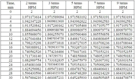
Finally, to show good convergence of our obtained results when terms tend to in…nity, we calculate c(t)for x=1 (Table 5). As it can be clearly seen, three terms approximations are su¢ cient to reach exact solutions.
Table 5. Results of HPM for C(t) for x = 1 versus time.
6. Final remarks
In this paper, the homotopy perturbation method (HPM) has been successfully implemented to solve the nonlinear system of di¤erential equations governing the ozone decomposition in aqueous solutions equations with initial condition. In conclusion, HPM provides highly accurate numerical solutions for nonlinear problems in comparison with other methods. The approximations are valid not only for small parameters but also for bigger ones and the initial approximation can be arbitrarily chosen with unknown constants which can be de…ned through di¤erent methods. As it is mentioned, HPM avoids linearization and physically unrealistic assumptions. Finally, comparisons with Adomian’s decomposition method reveals that the approximate solutions obtained from the HPM converge to their exact solutions faster than those of Adomian’s method (ADM). For computations Maple Package has been used.
References
1. A. Coely, A., Backlund and Darboux Transformations, (2001) American Math-ematical Society, Providence, Rhode Island.
2. Hirota., R., (1971), “Exact Solution of the Korteweg— de Vries Equation for Multiple Collisions of Solitons”, Physical Review Letter, 27, 1192-1194.
3. Malfeit, W., (1992), W., “Solitary wave solutions of nonlinear wave equations”, American Journal of Physics, 60- 650-657.
4. C.T. Yan, (1996), A simple transformation for nonlinear waves, Physics Letter A. 224, 77-84.
5. Yan, Z.Y., Zhang, H.Q., (2000), “On a new algorithm of constructing solitary wave solutions for systems of nonlinear evolution equations in mathematical physics”, Applied Mathematics and Mechanics. 21, 383-388.
6. Kaya, D., (2006), “An application for the higher order modi…ed KdV equa-tion by decomposiequa-tion method”, Communicaequa-tions in Nonlinear Science and Numerical Simulation, 10, 693–702.
7. Kaya, D., Elsayed, S.M., (2003), “On the solution of the coupled Schrödinger– KdV equation by the decomposition method”, Physics Letter A. 313, 82-88.
8. Al–Khalled, K., F Allan, F., (2004), “Construction of solutions for the shal-low water equations by the decomposition method”, Mathematics and Computers in Simulation, 66, 479–486.
9. He, J.H., (1999), “Homotopy perturbation technique”, Communications in Non-linear Science and Numerical Simulation, 178, 257–262.
10. Ganji, D.D., Rajabi, A., (2006) “Assessment of homotopy–perturbation and perturbation methods in heat radiation equations”, International Communications in Heat and Mass Transfer, 33, 391–400.
11. He, J.H., (2000), “A coupling method of a homotopy technique and a perturba-tion technique for non–linear problems”, Internaperturba-tional Journal of non-linear Nonlinear Mechanics, 35, 37–43.
12. He, J.H., (2005), “Limit cycle and bifurcation of nonlinear problems”, Chaos, Solitons Fractals, 26, 827–833.
13. He, J.H., (2005), “Homotopy perturbation method for bifurcation of nonlinear problems”, International Journal Nonlinear Science and Numerical Simulation, 6, 207– 208.
14. Barari, A., Omidvar, M., Ghotbi, Abdol, R,. Ganji. D.D., (2008), “Applica-tion of homotopy perturba“Applica-tion method and varia“Applica-tional itera“Applica-tion method to nonlinear oscillator di¤erential equations”, Acta Applicandae Mathematicae, 104, 161-171.
15. Barari, A., Omidvar, M., Ganji, D.D., Tahmasebi poor, A., (2008), “An approximate solution for boundary value problems in structural engineering and ‡uid mechanics”, Journal of Mathematical Problems in Engineering, Article ID 394103, 1-13.
16. Biazar, J., Tango, M., Islam, R., (2006), “Ozone decomposition of the second order in aqueous solutions”, Applied Mathematics and Computation, 177, 220–225.