Inverse Coefficient Problem of the Parabolic Equation with Periodic Boundary and Integral Overdetermination Conditions

(1)

Volume 2013, Article ID 659804,7pages http://dx.doi.org/10.1155/2013/659804

Research Article

Inverse Coefficient Problem of the Parabolic Equation with

Periodic Boundary and Integral Overdetermination Conditions

Fatma Kanca

Department of Management Information Systems, Kadir Has University, 34083 Istanbul, Turkey

Correspondence should be addressed to Fatma Kanca; fatma.kanca@khas.edu.tr Received 6 May 2013; Accepted 23 August 2013

Academic Editor: Daniel C. Biles

Copyright © 2013 Fatma Kanca. This is an open access article distributed under the Creative Commons Attribution License, which permits unrestricted use, distribution, and reproduction in any medium, provided the original work is properly cited.

This paper investigates the inverse problem of finding a time-dependent diffusion coefficient in a parabolic equation with the periodic boundary and integral overdetermination conditions. Under some assumption on the data, the existence, uniqueness, and continuous dependence on the data of the solution are shown by using the generalized Fourier method. The accuracy and computational efficiency of the proposed method are verified with the help of the numerical examples.

1. Introduction

Denote the domain𝐷_𝑇by

𝐷𝑇= {(𝑥, 𝑡) : 0 < 𝑥 < 1, 0 < 𝑡 ≤ 𝑇} . (1)

Consider the equation

𝑢_𝑡= 𝑎 (𝑡) 𝑢𝑥𝑥+ 𝐹 (𝑥, 𝑡) , (2)

with the initial condition

𝑢 (𝑥, 0) = 𝜑 (𝑥) , 0 ≤ 𝑥 ≤ 1, (3) the periodic boundary condition

𝑢 (0, 𝑡) = 𝑢 (1, 𝑡) , 𝑢_𝑥(0, 𝑡) = 𝑢_𝑥(1, 𝑡) ,

0 ≤ 𝑡 ≤ 𝑇, (4)

and the overdetermination condition ∫1

0 𝑥𝑢 (𝑥, 𝑡) 𝑑𝑥 = 𝐸 (𝑡) , 0 ≤ 𝑡 ≤ 𝑇. (5)

The problem of finding a pair{𝑎(𝑡), 𝑢(𝑥, 𝑡)} in (2)–(5) will be called an inverse problem.

Definition 1. The pair{𝑎(𝑡), 𝑢(𝑥, 𝑡)} from the class 𝐶[0, 𝑇] ×

𝐶2,1_(𝐷

𝑇) ∩ 𝐶1,0(𝐷𝑇) for which conditions (2)–(5) is satisfied

and𝑎(𝑡) > 0 on the interval [0, 𝑇], is called a classical solution of the inverse problem (2)–(5).

The parameter identification in a parabolic differential equation from the data of integral overdetermination condi-tion plays an important role in engineering and physics [1–7]. This integral condition in parabolic problems is also called heat moments [5].

Boundary value problems for parabolic equations in one or two local classical conditions are replaced by heat moments [8–13]. These kinds of conditions such as (5) arise from many important applications in heat transfer, thermoelasticity, control theory, life sciences, and so forth. For example, in heat propagation in a thin rod, the law of variation𝐸(𝑡) of the total quantity of heat in the rod is given in [8]. In [12], a physical-mechanical interpretation of the integral conditions was also given.

Various statements of inverse problems on determination of thermal coefficient in one-dimensional heat equation were studied in [4,5,7,14]. In papers [4,5,7], the time-dependent thermal coefficient is determined from the heat moment.

Boundary value problems and inverse problems for parabolic equations with periodic boundary conditions are investigated in [15,16].

(2)

In the present work, one heat moment is used with peri-odic boundary condition for the determination of thermal coefficient. The existence and uniqueness of the classical solution of the problem (2)–(5) is reduced to fixed point principles by applying the Fourier method.

This paper organized as follows. In Section 2, the exis-tence and uniqueness of the solution of inverse problem (2)– (5) are proved by using the Fourier method. In Section 3, the continuous dependence on the solution of the inverse problem is shown. InSection 4, the numerical procedure for the solution of the inverse problem using the Crank-Nicolson scheme combined with an iteration method is given. Finally, inSection 5, numerical experiments are presented and dis-cussed.

2. Existence and Uniqueness of

the Solution of the Inverse Problem

We have the following assumptions on the data of the problem (2)–(5). (𝐴₁)𝐸(𝑡) ∈ 𝐶1[0, 𝑇], 𝐸󸀠(𝑡) > 0, for all 𝑡 ∈ [0, 𝑇]; (𝐴₂)𝜑(𝑥) ∈ 𝐶4[0, 1]; (1)𝜑(0) = 𝜑(1), 𝜑󸀠(0) = 𝜑󸀠(1), 𝜑󸀠󸀠(0) = 𝜑󸀠󸀠(1), ∫₀1𝑥𝜑(𝑥)𝑑𝑥 = 𝐸(0); (2)𝜑_𝑛≥ 0, 𝑛 = 1, 2, . . .;

(𝐴₃)𝐹(𝑥, 𝑡) ∈ 𝐶(𝐷_𝑇); 𝐹(𝑥, 𝑡) ∈ 𝐶4[0, 1] for arbitrary fixed 𝑡 ∈ [0, 𝑇];

(1)𝐹(0, 𝑡) = 𝐹(1, 𝑡), 𝐹_𝑥(0, 𝑡) = 𝐹_𝑥(1, 𝑡), 𝐹_𝑥𝑥(0, 𝑡) = 𝐹_𝑥𝑥(1, 𝑡);

(2)𝐹_𝑛(𝑡) ≥ 0, 𝑛 = 1, 2, . . .,

where𝜑_𝑛=∫₀1𝜑(𝑥) sin(2𝜋𝑛𝑥)𝑑𝑥, 𝐹_𝑛(𝑡)=∫₀1𝐹(𝑥, 𝑡) sin(2𝜋𝑛𝑥)𝑑𝑥, 𝑛 = 0, 1, 2, . . . .

Theorem 2. Let the assumptions (𝐴₁)–(𝐴₃) be satisfied. Then the following statements are true.

(1) The inverse problem (2)–(5) has a solution in𝐷_𝑇.

(2) The solution of inverse problem (2)–(5) is unique in 𝐷_𝑇₀, where the number𝑇₀(0 < 𝑇₀ < 𝑇) is determined by the data of the problem.

Proof. By applying the standard procedure of the Fourier

method, we obtain the following representation for the solu-tion of (2)–(4) for arbitrary𝑎(𝑡) ∈ 𝐶[0, 𝑇]:

𝑢 (𝑥, 𝑡) = ∑∞ 𝑛=1 [𝜑_𝑛𝑒−(2𝜋𝑛)2∫0𝑡𝑎(𝑠)𝑑𝑠+ ∫ 𝑡 0𝐹𝑛(𝜏) 𝑒 −(2𝜋𝑛)2_∫𝑡 𝜏𝑎(𝑠)𝑑𝑠𝑑𝜏] × sin (2𝜋𝑛𝑥) . (6) The assumptions𝜑(0) = 𝜑(1), 𝜑󸀠(0) = 𝜑󸀠(1), 𝐹(0, 𝑡) = 𝐹(1, 𝑡), and 𝐹_𝑥(0, 𝑡) = 𝐹_𝑥(1, 𝑡) are consistent conditions for the representation (2) of the solution𝑢(𝑥, 𝑡) to be valid. Further-more, under the smoothness assumptions𝜑(𝑥) ∈ 𝐶4[0, 1],

𝐹(𝑥, 𝑡) ∈ 𝐶(𝐷_𝑇), and 𝐹(𝑥, 𝑡) ∈ 𝐶4_{[0, 1] for all 𝑡 ∈ [0, 𝑇], the}

series (6) and its𝑥-partial derivative converge uniformly in 𝐷_𝑇 since their majorizing sums are absolutely convergent. Therefore, their sums𝑢(𝑥, 𝑡) and 𝑢_𝑥(𝑥, 𝑡) are continuous in 𝐷_𝑇. In addition, the𝑡-partial derivative and the 𝑥𝑥-second-order partial derivative series are uniformly convergent for 𝑡 ≥ 𝜀 > 0 (𝜀 is an arbitrary positive number). Thus, 𝑢(𝑥, 𝑡) ∈ 𝐶2,1_(𝐷

𝑇) ∩ 𝐶1,0(𝐷𝑇) and satisfies the conditions (2)–(4). In

addition,𝑢_𝑡(𝑥, 𝑡) is continuous in 𝐷_𝑇because the majorizing sum of 𝑡-partial derivative series is absolutely convergent under the condition𝜑󸀠󸀠(0) = 𝜑󸀠󸀠(1) and 𝑓_𝑥𝑥(0, 𝑡) = 𝑓_𝑥𝑥(1, 𝑡) in𝐷_𝑇. Equation (6) can be differentiated under the condition (𝐴₁) to obtain

∫1

0 𝑥𝑢𝑡(𝑥, 𝑡) 𝑑𝑥 = 𝐸

󸀠_{(𝑡) ,} ₍₇₎

and this yields

𝑎 (𝑡) = 𝑃 [𝑎 (𝑡)] , (8) where 𝑃 [𝑎 (𝑡)] = 𝐸󸀠(𝑡) + ∑∞𝑛=1(1/2𝜋𝑛) 𝐹𝑛(𝑡) ∑∞_𝑛=12𝜋𝑛 (𝜑_𝑛𝑒−(2𝜋𝑛)2_∫𝑡 0𝑎(𝑠)𝑑𝑠+ ∫𝑡 0𝐹𝑛(𝜏) 𝑒−(2𝜋𝑛) 2_∫𝑡 𝜏𝑎(𝑠)𝑑𝑠𝑑𝜏) . (9) Denote 𝐶₀= min 𝑡∈[0,𝑇]𝐸 󸀠_{(𝑡) + min} 𝑡∈[0,𝑇]( ∞ ∑ 𝑛=1 1 2𝜋𝑛𝐹𝑛(𝑡)) , 𝐶₁= max 𝑡∈[0,𝑇]𝐸 󸀠_{(𝑡) + max} 𝑡∈[0,𝑇]( ∞ ∑ 𝑛=1 1 2𝜋𝑛𝐹𝑛(𝑡)) , 𝐶₂= 𝐸󸀠(0) , 𝐶₃=∑∞ 𝑘=1 2𝜋𝑛 (𝜑_𝑛+ ∫𝑇 0 𝐹𝑛(𝜏) 𝑑𝜏) . (10) Using the representation (8), the following estimate is true:

0 < 𝐶0

𝐶₃ ≤ 𝑎 (𝑡) ≤ 𝐶₁

𝐶₂. (11)

Introduce the set𝑀 as

𝑀 = {𝑎 (𝑡) ∈ 𝐶 [0, 𝑇] : 𝐶0

C₃ ≤ 𝑎 (𝑡) ≤ 𝐶₁

𝐶₂} . (12) It is easy to see that

𝑃 : 𝑀 󳨀→ 𝑀. (13)

Compactness of𝑃 is verified by analogy to [7]. By virtue of Schauder’s fixed-point theorem, we have a solution𝑎(𝑡) ∈ 𝐶[0, 𝑇] of (8).

Now let us show that there exists𝐷_𝑇₀ (0 < 𝑇₀ ≤ 𝑇) for which the solution(𝑎, 𝑢) of the problem (2)–(5) is unique in

(3)

𝐷_𝑇₀. Suppose that(𝑏, V) is also a solution pair of the problem (2)–(5). Then from the representations (6) and (8) of the solution, we have 𝑢 (𝑥, 𝑡) − V (𝑥, 𝑡) =∑∞ 𝑛=1𝜑𝑛(𝑒 −(2𝜋𝑛)2_∫𝑡 0𝑎(𝑠)𝑑𝑠− 𝑒−(2𝜋𝑛)2∫ 𝑡 0𝑏(𝑠)𝑑𝑠) sin 2𝜋𝑛 (𝑥) +∑∞ 𝑛=1(∫ 𝑡 0𝐹𝑛(𝜏) (𝑒 −(2𝜋𝑛)2_∫𝑡 𝜏𝑎(𝑠)𝑑𝑠− 𝑒−(2𝜋𝑛)2∫ 𝑡 𝜏𝑏(𝑠)𝑑𝑠) 𝑑𝜏) × sin 2𝜋𝑛 (𝑥) , 𝑎 (𝑡) − 𝑏 (𝑡) = 𝑃 [𝑎 (𝑡)] − 𝑃 [𝑏 (𝑡)] , (14) where 𝑃 [𝑎 (𝑡)] − 𝑃 [𝑏 (𝑡)] = 𝐸󸀠(𝑡) + ∑∞𝑛=1(1/2𝜋𝑛) 𝐹𝑛(𝑡) ∑∞_𝑛=12𝜋𝑛 (𝜑_𝑛𝑒−(2𝜋𝑛)2_∫𝑡 0𝑎(𝑠)𝑑𝑠+ ∫𝑡 0𝐹𝑛(𝜏) 𝑒−(2𝜋𝑛) 2_∫𝑡 𝜏𝑎(𝑠)𝑑𝑠𝑑𝜏) − 𝐸󸀠(𝑡) + ∑∞𝑛=1(1/2𝜋𝑛) 𝐹𝑛(𝑡) ∑∞_𝑛=12𝜋𝑛 (𝜑_𝑛𝑒−(2𝜋𝑛)2_∫𝑡 0𝑏(𝑠)𝑑𝑠+ ∫𝑡 0𝐹𝑛(𝜏) 𝑒−(2𝜋𝑛) 2_∫𝑡 𝜏𝑏(𝑠)𝑑𝑠𝑑𝜏) . (15) The following estimate is true:

|𝑃 [𝑎 (𝑡)] − 𝑃 [𝑏 (𝑡)]| ≤ (𝐸 󸀠_{(𝑡) + ∑}∞ 𝑛=1(1/2𝜋𝑛) 𝐹𝑛(𝑡)) 𝐶2 2 ⋅ (∑∞ 𝑛=1 2𝜋𝑛𝜑_𝑛(𝑒−(2𝜋𝑛)2∫0𝑡𝑎(𝑠)𝑑𝑠− 𝑒−(2𝜋𝑛)2∫ 𝑡 0𝑏(𝑠)𝑑𝑠) + ∞ ∑ 𝑛=1 2𝜋𝑛 × (∫𝑡 0𝐹𝑛(𝜏) (𝑒 −(2𝜋𝑛)2_∫𝑡 𝜏𝑎(𝑠)𝑑𝑠− 𝑒−(2𝜋𝑛)2∫ 𝑡 𝜏𝑏(𝑠)𝑑𝑠) 𝑑𝜏)) . (16) Using the estimates

Let𝛼 ∈ (0, 1) be arbitrary fixed number. Fix a number 𝑇₀, 0 < 𝑇₀≤ 𝑇, such that

𝐶₁(𝐶₄+ 𝐶₅) 𝐶2

2 𝑇0≤ 𝛼.

(19)

Then from the equality (10), we obtain

‖𝑎 − 𝑏‖_𝐶[0,𝑇₀_]≤ 𝛼‖𝑎 − 𝑏‖𝐶[0,𝑇0], (20)

which implies that𝑎 = 𝑏. By substituting 𝑎 = 𝑏 in (9), we have 𝑢 = V.

3. Continuous Dependence of

(𝑎, 𝑢) on the Data

Theorem 3. Under assumptions (𝐴1)–(𝐴3), the solution(𝑎, 𝑢)

of the problem (2)–(5) depends continuously on the data for

small T.

Proof. LetΦ = {𝜑, 𝐹, 𝐸} and Φ = {𝜑, 𝐹, 𝐸} be two sets of the

data, which satisfy the assumptions (𝐴₁)–(𝐴₃). Then there exist positive constants𝑀_𝑖,𝑖 = 1,2,3 such that

󵄩󵄩󵄩󵄩𝜑󵄩󵄩󵄩󵄩𝐶4_[0,1]≤ 𝑀₁, ‖𝐹‖_𝐶4,0_(𝐷 𝑇)≤ 𝑀2, ‖𝐸‖𝐶1_[0,𝑇]≤ 𝑀₃, 󵄩󵄩󵄩󵄩𝜑󵄩󵄩󵄩󵄩𝐶4_[0,1]≤ 𝑀₁, 󵄩󵄩󵄩󵄩 󵄩𝐹󵄩󵄩󵄩󵄩󵄩𝐶4,0_(𝐷 𝑇)≤ 𝑀2, 󵄩󵄩󵄩󵄩 󵄩𝐸󵄩󵄩󵄩󵄩󵄩𝐶1_[0,𝑇]≤ 𝑀3. (21)

Let(𝑎, 𝑢) and (𝑎, 𝑢) be solutions of the inverse problem (2)–(5) corresponding to the dataΦ and Φ, respectively. Ac-cording to (8), 𝑎 (𝑡) = 𝐸󸀠(𝑡) + ∑∞𝑛=1(1/2𝜋𝑛) 𝐹𝑛(𝑡) ∑∞_𝑛=12𝜋𝑛 (𝜑_𝑛𝑒−(2𝜋𝑛)2_∫𝑡 0𝑎(𝑠)𝑑𝑠+ ∫𝑡 0𝐹𝑛(𝜏) 𝑒−(2𝜋𝑛) 2_∫𝑡 𝜏𝑎(𝑠)𝑑𝑠𝑑𝜏) , 𝑎 (𝑡) = 𝐸 󸀠_{(𝑡) + ∑}∞ 𝑛=1(1/2𝜋𝑛) 𝐹𝑛(𝑡) ∑∞_𝑛=12𝜋𝑛 (𝜑_𝑛𝑒−(2𝜋𝑛)2_∫𝑡 0𝑎(𝑠)𝑑𝑠+ ∫𝑡 0𝐹𝑛(𝜏) 𝑒−(2𝜋𝑛) 2_∫𝑡 𝜏𝑎(𝑠)𝑑𝑠𝑑𝜏) . (22)

(4)

First let us estimate the difference𝑎 − 𝑎. It is easy to compute that 󵄨󵄨󵄨󵄨 󵄨󵄨󵄨󵄨 󵄨󵄨𝐸 󸀠_(𝑡)_∑∞ 𝑛=1 2𝜋𝑛𝜑_𝑛𝑒−(2𝜋𝑛)2∫0𝑡𝑎(𝑠)𝑑𝑠 −𝐸󸀠(𝑡)∑∞ 𝑛=1 2𝜋𝑛𝜑_𝑛𝑒−(2𝜋𝑛)2_∫𝑡 0𝑎(𝑠)𝑑𝑠󵄨󵄨󵄨󵄨󵄨󵄨󵄨󵄨 󵄨󵄨 ≤ 𝑀₄󵄩󵄩󵄩󵄩_{󵄩𝐸 − 𝐸}󵄩󵄩󵄩󵄩_󵄩_𝐶1_[0,𝑇]+ 𝑀5󵄩󵄩󵄩󵄩𝜑 − 𝜑󵄩󵄩󵄩󵄩𝐶4_[0,1] + 𝑀₆‖𝑎 − 𝑎‖_𝐶[0,𝑇], 󵄨󵄨󵄨󵄨 󵄨󵄨󵄨󵄨 󵄨󵄨𝐸 󸀠_(𝑡)_∑∞ 𝑛=1 2𝜋𝑛 ∫𝑡 0𝐹𝑛(𝜏) 𝑒 −(2𝜋𝑛)2_∫𝑡 𝜏𝑎(𝑠)𝑑𝑠𝑑𝜏 −𝐸󸀠(𝑡)∑∞ 𝑛=12𝜋𝑛 ∫ 𝑡 0𝐹𝑛(𝜏) 𝑒 −(2𝜋𝑛)2_∫𝑡 𝜏𝑎(𝑠)𝑑𝑠𝑑𝜏󵄨󵄨󵄨󵄨󵄨󵄨󵄨󵄨 󵄨󵄨 ≤ 𝑀₇_{𝑇󵄩󵄩󵄩󵄩󵄩𝐸 − 𝐸}󵄩󵄩󵄩󵄩_󵄩_𝐶1_[0,𝑇]+ 𝑀5𝑇󵄩󵄩󵄩󵄩󵄩𝐹 − 𝐹󵄩󵄩󵄩󵄩󵄩 𝐶4,0(𝐷𝑇) + 𝑀₈‖𝑎 − 𝑎‖_𝐶[0,𝑇], 󵄨󵄨󵄨󵄨 󵄨󵄨󵄨󵄨 󵄨󵄨 ∞ ∑ 𝑛=1 1 2𝜋𝑛𝐹𝑛(𝑡) ∞ ∑ 𝑛=1 2𝜋𝑛𝜑_𝑛𝑒−(2𝜋𝑛)2∫0𝑡𝑎(𝑠)𝑑𝑠 −∑∞ 𝑛=1 1 2𝜋𝑛𝐹𝑛(𝑡) ∞ ∑ 𝑛=1 2𝜋𝑛𝜑_𝑛𝑒−(2𝜋𝑛)2∫0𝑡𝑎(𝑠)𝑑𝑠󵄨󵄨󵄨󵄨󵄨󵄨󵄨󵄨 󵄨󵄨 ≤ 2√6𝑀₄󵄩󵄩󵄩󵄩_{󵄩𝐹 − 𝐹}󵄩󵄩󵄩󵄩_󵄩_𝐶4,0_(𝐷 𝑇)+ 2√6𝑀7󵄩󵄩󵄩󵄩𝜑 − 𝜑󵄩󵄩󵄩󵄩𝐶4[0,1] + 𝑀₉‖𝑎 − 𝑎‖_𝐶[0,𝑇], 󵄨󵄨󵄨󵄨 󵄨󵄨󵄨󵄨 󵄨󵄨 ∞ ∑ 𝑛=1 1 2𝜋𝑛𝐹𝑛(𝑡) ∞ ∑ 𝑛=12𝜋𝑛 ∫ 𝑡 0𝐹𝑛(𝜏) 𝑒 −(2𝜋𝑛)2_∫𝑡 𝜏𝑎(𝑠)𝑑𝑠 −∑∞ 𝑛=1 1 2𝜋𝑛𝐹𝑛(𝑡) ∞ ∑ 𝑛=1 2𝜋𝑛 ∫𝑡 0𝐹𝑛(𝜏) 𝑒 −(2𝜋𝑛)2_∫𝑡 𝜏𝑎(𝑠)𝑑𝑠𝑑𝜏󵄨󵄨󵄨󵄨󵄨󵄨󵄨󵄨 󵄨󵄨 ≤ √6𝑇𝑀󵄩󵄩󵄩󵄩󵄩𝐹 − 𝐹󵄩󵄩󵄩󵄩󵄩𝐶4,0_(𝐷 𝑇)+ 𝑀10‖𝑎 − 𝑎‖𝐶[0,𝑇], (23) where𝑀_𝑘,𝑘 = 4, . . . , 10, are some constants.

If we consider these estimates in𝑎 − 𝑎, we obtain (1 − 𝑀₁₁) ‖𝑎 − 𝑎‖𝐶[0,𝑇]

≤ 𝑀₁₂_{(󵄩󵄩󵄩󵄩󵄩𝐸 − 𝐸}󵄩󵄩󵄩󵄩_󵄩_𝐶1_[0,𝑇]+ 󵄩󵄩󵄩󵄩𝜑 − 𝜑󵄩󵄩󵄩󵄩_𝐶4_[0,1]+ 󵄩󵄩󵄩󵄩󵄩𝐹 − 𝐹󵄩󵄩󵄩󵄩_󵄩_𝐶4,0_(𝐷 𝑇)) .

(24) The inequality𝑀₁₁< 1 holds for small 𝑇. Finally, we obtain

‖𝑎 − 𝑎‖𝐶[0,𝑇]≤ 𝑀13󵄩󵄩󵄩󵄩_{󵄩Φ − Φ}󵄩󵄩󵄩󵄩_{󵄩 , 𝑀}13=_{(1 − 𝑀}𝑀12 11), (25) where ‖Φ − Φ‖ = ‖𝐸 − 𝐸‖_𝐶1_[0,𝑇] + ‖𝜑 − 𝜑‖_𝐶4_[0,1] + ‖𝐹 − 𝐹‖_𝐶4,0_(𝐷 𝑇).

From (6), a similar estimate is also obtained for the dif-ference𝑢 − 𝑢 as

‖𝑢 − 𝑢‖_𝐶(𝐷_𝑇₎≤ 𝑀₁₄󵄩󵄩󵄩󵄩_{󵄩Φ − Φ}󵄩󵄩󵄩󵄩_{󵄩 .} (26)

4. Numerical Method

We use the finite difference method with a predictor-correct-or-type approach, that is suggested in [2]. Apply this method to the problem (2)–(5).

We subdivide the intervals[0, 1] and [0, 𝑇] into 𝑁_𝑥and 𝑁_𝑡subintervals of equal lengthsℎ = (1/𝑁_𝑥) and 𝜏 = (𝑇/𝑁_𝑡), respectively. Then we add two lines𝑥 = 0 and 𝑥 = (𝑁_𝑥+ 1)ℎ to generate the fictitious points needed for dealing with the second boundary condition. We choose the Crank-Nicolson scheme, which is absolutely stable and has a second-order accuracy in bothℎ and 𝜏 [15]. The Crank-Nicolson scheme for (2)–(5) is as follows: 1 𝜏(𝑢𝑗+1𝑖 − 𝑢𝑗𝑖) = 1 2(𝑎𝑗+1+ 𝑎𝑗) 1 2ℎ2 × [(𝑢𝑗_𝑖−1− 2𝑢𝑗_𝑖 + 𝑢𝑗_𝑖+1) + (𝑢𝑗+1_𝑖−1 − 2𝑢𝑗+1_𝑖 + 𝑢𝑗+1_𝑖+1)] +1 2(𝐹𝑖𝑗+1+ 𝐹𝑖𝑗) , 𝑢0_𝑖 = 𝜙_𝑖, 𝑢𝑗₀= 𝑢𝑗_𝑁_𝑥, 𝑢𝑗₁= 𝑢𝑗_𝑁_𝑥₊₁, (27) where1 ≤ 𝑖 ≤ 𝑁_𝑥and0 ≤ 𝑗 ≤ 𝑁_𝑡are the indices for the spatial and time steps, respectively,𝑢𝑗_𝑖 = 𝑢(𝑥_𝑖, 𝑡_𝑗), 𝜙_𝑖= 𝜑(𝑥_𝑖), 𝐹_𝑖𝑗 = 𝐹(𝑥_𝑖, 𝑡_𝑗), and 𝑥_𝑖 = 𝑖ℎ, 𝑡_𝑗 = 𝑗𝜏. At the 𝑡 = 0 level, adjustment should be made according to the initial condition and the compatibility requirements.

Equation (27) form an𝑁_𝑥×𝑁_𝑥linear system of equations

𝐴𝑈𝑗+1_{= 𝑏,} ₍₂₈₎ where 𝑈𝑗 = (𝑢𝑗₁, 𝑢𝑗₂, . . . , 𝑢𝑗_𝑁 𝑥) tr , 1 ≤ 𝑗 ≤ 𝑁_𝑡, 𝑏 = (𝑏₁, 𝑏₂, . . . , 𝑏_𝑁_𝑥)tr, 𝐴= [ [ [ [ [ [ [ [ [ −2 (1 + 𝑅) 1 0 ⋅ ⋅ ⋅ 0 1 1 −2 (1 + 𝑅) 1 0 ⋅ ⋅ ⋅ 0 0 1 −2 (1 + 𝑅) 1 0 ⋅ ⋅ ⋅ 0 . . . d 0 1 −2 (1 + 𝑅) 1 1 0 1 −2 (1 + 𝑅) ] ] ] ] ] ] ] ] ] ,

(5)

𝑅 = 2ℎ2 𝜏 (𝑎𝑗+1_{+ 𝑎}𝑗₎, 𝑗 = 0, 1, . . . , 𝑁𝑡, 𝑏₁= 2 (1 − 𝑅) 𝑢𝑗₁− 𝑢𝑗₂− 𝑢𝑗_𝑁_𝑥− 𝑅𝜏 (𝐹₁𝑗+1+ 𝐹₁𝑗) , 𝑗 = 0, 1, . . . , 𝑁_𝑡, 𝑏_𝑁_𝑥 = − 𝑢𝑗_𝑁_𝑥₋₁+ 2 (1 − 𝑅) 𝑢𝑗_𝑁_𝑥− 𝑢𝑗₁ − 𝑅𝜏 (𝐹_𝑁𝑗+1_𝑥 + 𝐹_𝑁𝑗_𝑥) , 𝑗 = 0, 1, . . . , 𝑁_𝑡, 𝑏𝑖= − 𝑢𝑗𝑖−1+ 2 (1 − 𝑅) 𝑢𝑗𝑖− 𝑢𝑗𝑖+1− 𝑅𝜏 (𝐹𝑖𝑗+1+ 𝐹𝑖𝑗) , 𝑖 = 2, 3, . . . , 𝑁𝑥− 1, 𝑗 = 0, 1, . . . , 𝑁𝑡. (29) Now, let us construct the predicting-correcting mecha-nism. First, multiplying (2) by 𝑥 from 0 to 1 and using (4) and (5), we obtain

𝑎 (𝑡) = 𝐸

󸀠_{(𝑡) − ∫}1

0𝑥𝐹 (𝑥, 𝑡) 𝑑𝑥

𝑢_𝑥(1, 𝑡) . (30) The finite difference approximation of (30) is

𝑎𝑗 = [((𝐸 𝑗+1_{− 𝐸}𝑗_{) /𝜏) − (Fin)}𝑗_{] ℎ} 𝑢𝑗_𝑁_𝑥₊₁− 𝑢𝑗_𝑁_𝑥 , (31) where𝐸𝑗 = 𝐸(𝑡_𝑗), (Fin)𝑗 = ∫₀1𝑥𝐹(𝑥, 𝑡_𝑗)𝑑𝑥, 𝑗 = 0, 1, . . . , 𝑁_𝑡. For𝑗 = 0, 𝑎0= [((𝐸 1_{− 𝐸}0_{) /𝜏) − (Fin)}0_{] ℎ} 𝜙_𝑁_𝑥₊₁− 𝜙_𝑁_𝑥 , (32) and the values of𝜙_𝑖 help us to start our computation. We denote the values of𝑎𝑗, 𝑢𝑗_𝑖 at the𝑠th iteration step 𝑎𝑗(𝑠), 𝑢𝑗(𝑠)_𝑖 , respectively. In numerical computation, since the time step is very small, we can take𝑎𝑗+1(0) = 𝑎𝑗, 𝑢𝑗+1(0)_𝑖 = 𝑢𝑗_𝑖, 𝑗 = 0, 1, 2, . . . 𝑁_𝑡,𝑖 = 1, 2, . . . , 𝑁_𝑥. At each(𝑠 + 1)th iteration step, we first determine𝑎𝑗+1(𝑠+1)from the formula

𝑎𝑗+1(𝑠+1)=[((𝐸

𝑗+2_{− 𝐸}𝑗+1_{) /𝜏) − (Fin)}𝑗+1_{] ℎ}

𝑢𝑗+1(𝑠)_𝑁_𝑥₊₁ − 𝑢𝑗+1(𝑠)_𝑁_𝑥 . (33) Then from (27) we obtain

1 𝜏(𝑢𝑖𝑗+1(𝑠+1)− 𝑢𝑗+1(𝑠)𝑖 ) = 1 4ℎ2(𝑎𝑗+1(𝑠+1)+ 𝑎𝑗+1(𝑠)) × [(𝑢𝑗+1(𝑠+1)_𝑖−1 − 2𝑢𝑗+1(𝑠+1)_𝑖 + 𝑢𝑗+1(𝑠+1)_𝑖+1 ) + (𝑢𝑗+1(𝑠)_𝑖−1 − 2𝑢𝑗+1(𝑠)_𝑖 + 𝑢𝑗+1(𝑠)_𝑖+1 )] +1 2(𝐹𝑖𝑗+1+ 𝐹𝑖𝑗) , 𝑢𝑗+1(𝑠)₀ = 𝑢𝑗+1(𝑠)_𝑁_𝑥 , 𝑢₁𝑗+1(𝑠)= 𝑢𝑗+1(𝑠)_𝑁 𝑥+1, 𝑠 = 0, 1, 2, . . . . (34) 0 0.2 0.4 0.6 0.8 1 1 2 3 4 5 6 7 8 t a(t)

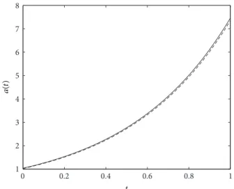
Figure 1: The analytical and numerical solutions of𝑎(𝑡) when 𝑇 = 1. The analytical solution is shown with dashed line.

0 0.2 0.4 0.6 0.8 1 −0.4 −0.3 −0.2 −0.1 0 0.1 0.2 0.3 0.4 t u( x, t)

Figure 2: The analytical and numerical solutions of𝑢(𝑥, 𝑡) at the 𝑇 = 1. The analytical solution is shown with dashed line.

The system of (34) can be solved by the Gauss elimination method and𝑢𝑗+1(𝑠+1)_𝑖 is determined. If the difference of values between two iterations reaches the prescribed tolerance, the iteration is stopped and we accept the corresponding values 𝑎𝑗+1(𝑠+1)_, _𝑢𝑗+1(𝑠+1)

𝑖 (𝑖 = 1, 2, . . . , 𝑁𝑥) as 𝑎𝑗+1, 𝑢𝑗+1𝑖 (𝑖 =

1, 2, . . . , 𝑁_𝑥), on the (𝑗 + 1)th time step, respectively. In virtue of this iteration, we can move from level𝑗 to level 𝑗 + 1.

5. Numerical Examples and Discussions

Example 1. Consider the inverse problem (2)–(5), with 𝐹 (𝑥, 𝑡) = (2𝜋)2sin(2𝜋𝑥) exp (𝑡) ,

𝜑 (𝑥) = sin (2𝜋𝑥) , 𝐸 (𝑡) = −_2𝜋1 exp(−𝑡) , 𝑥 ∈ [0, 1] , 𝑡 ∈ [0, 𝑇] .

(6)

0 0.2 0.4 0.6 0.8 1 0 0.5 1 1.5 2 2.5 3 t a(t)

Figure 3: The analytical and numerical solutions of𝑎(𝑡) when 𝑇 = 1. The analytical solution is shown with dashed line.

0 0.2 0.4 0.6 0.8 1 −0.4 −0.3 −0.2 −0.1 0 0.1 0.2 0.3 0.4 t u( x, t)

Figure 4: The analytical and numerical solutions of𝑢(𝑥, 𝑡) at the 𝑇 = 1. The analytical solution is shown with dashed line.

It is easy to check that the analytical solution of the prob-lem (2)–(5) is

{𝑎 (𝑡) , 𝑢 (𝑥, 𝑡)} = { 1

(2𝜋)2 + exp (2𝑡) , sin (2𝜋𝑥) exp (−𝑡)} . (36)

Let us apply the scheme which was explained in the previous section for the step sizesℎ = 0.005, 𝜏 = 0.005.

In the case when 𝑇 = 1, the comparisons between the analytical solution (36) and the numerical finite difference solution are shown in Figures1and2.

Example 2. Consider the inverse problem (2)–(5), with 𝐹 (𝑥, 𝑡) = (2𝜋)2sin(2𝜋𝑥) exp (−𝑡 + sin (4𝜋𝑡)) ,

𝜑 (𝑥) = sin (2𝜋𝑥) , 𝐸 (𝑡) = −_2𝜋1 exp(−𝑡) , 𝑥 ∈ [0, 1] , 𝑡 ∈ [0, 𝑇] .

(37)

It is easy to check that the analytical solution of the prob-lem (2)–(5) is

{𝑎 (𝑡) , 𝑢 (𝑥, 𝑡)} = { 1

(2𝜋)2 + exp (sin (4𝜋𝑡)) , sin (2𝜋𝑥) exp (−𝑡)} . (38)

Let us apply the scheme which was explained in the previous section for the step sizesℎ = 0.01, 𝜏 = ℎ/8.

In the case when 𝑇 = 1, the comparisons between the analytical solution (38) and the numerical finite difference solution are shown in Figures3and4.

6. Conclusions

The inverse problem regarding the simultaneously identi-fication of the time-dependent thermal diffusivity and the temperature distribution in one-dimensional heat equation with periodic boundary and integral overdetermination con-ditions has been considered. This inverse problem has been investigated from both theoretical and numerical points of view. In the theoretical part of the paper, the conditions for the existence, uniqueness, and continuous dependence on the data of the problem have been established. In the numerical part, the sensitivity of the Crank-Nicolson finite-difference scheme combined with an iteration method with the examples has been illustrated.

References

[1] J. R. Cannon, Y. P. Lin, and S. Wang, “Determination of a control parameter in a parabolic partial differential equation,”

The Journal of the Australian Mathematical Society B, vol. 33, no.

2, pp. 149–163, 1991.

[2] J. R. Cannon, Y. Lin, and S. Wang, “Determination of source parameter in parabolic equations,” Meccanica, vol. 27, no. 2, pp. 85–94, 1992.

[3] A. G. Fatullayev, N. Gasilov, and I. Yusubov, “Simultaneous determination of unknown coefficients in a parabolic equation,”

Applicable Analysis, vol. 87, no. 10-11, pp. 1167–1177, 2008.

[4] M. I. Ivanchov, “Inverse problems for the heat-conduction equation with nonlocal boundary condition,” Ukrainian

Math-ematical Journal, vol. 45, no. 8, pp. 1186–1192, 1993.

[5] M. I. Ivanchov and N. V. Pabyrivska, “Simultaneous determi-nation of two coefficients in a parabolic equation in the case of nonlocal and integral conditions,” Ukrainian Mathematical

Journal, vol. 53, no. 5, pp. 674–684, 2001.

[6] M. I. Ismailov and F. Kanca, “An inverse coefficient problem for a parabolic equation in the case of nonlocal boundary and overdetermination conditions,” Mathematical Methods in the

(7)

[7] F. Kanca and M. I. Ismailov, “The inverse problem of finding the time-dependent diffusion coefficient of the heat equation from integral overdetermination data,” Inverse Problems in Science

and Engineering, vol. 20, no. 4, pp. 463–476, 2012.

[8] J. R. Cannon, “The solution of the heat equation subject to the specification of energy,” Quarterly of Applied Mathematics, vol. 21, pp. 155–160, 1963.

[9] L. I. Kamynin, “A boundary value problem in the theory of heat conduction with a nonclassical boundary condition,” Zhurnal

Vychislitel’noi Matematiki i Matematicheskoi Fiziki, vol. 4, no. 6,

pp. 1006–1024, 1964.

[10] N. I. Ionkin, “Solution of a boundary-value problem in heat con-duction with a nonclassical boundary condition,” Differential

Equations, vol. 13, pp. 204–211, 1977.

[11] N. I. Yurchuk, “Mixed problem with an integral condition for certain parabolic equations,” Differential Equations, vol. 22, pp. 1457–1463, 1986.

[12] V. M. V¯ıgak, “Construction of a solution of the heat conduction problem with integral conditions,” Doklady Akademii Nauk

Ukrainy, vol. 8, pp. 57–60, 1994.

[13] N. I. Ivanchov, “Boundary value problems for a parabolic equa-tion with integral condiequa-tions,” Differential Equaequa-tions, vol. 40, no. 4, pp. 591–609, 2004.

[14] W. Liao, M. Dehghan, and A. Mohebbi, “Direct numerical method for an inverse problem of a parabolic partial differential equation,” Journal of Computational and Applied Mathematics, vol. 232, no. 2, pp. 351–360, 2009.

[15] I. Sakinc, “Numerical solution of a quasilinear parabolic prob-lem with periodic boundary condition,” Hacettepe Journal of

Mathematics and Statistics, vol. 39, no. 2, pp. 183–189, 2010.

[16] J. Choi, “Inverse problem for a parabolic equation with space-periodic boundary conditions by a Carleman estimate,” Journal

(8)

Submit your manuscripts at

http://www.hindawi.com

Hindawi Publishing Corporation

http://www.hindawi.com Volume 2014

Mathematics

Journal of

http://www.hindawi.com Volume 2014 Mathematical Problems in Engineering

Hindawi Publishing Corporation http://www.hindawi.com

Differential Equations

International Journal of

Volume 2014 Hindawi Publishing Corporation

http://www.hindawi.com Volume 2014 Hindawi Publishing Corporationhttp://www.hindawi.com Volume 2014

Mathematical PhysicsAdvances in

Complex Analysis

Journal of

Optimization

Journal of

Combinatorics

Journal of

Function Spaces

Abstract and Applied Analysis Hindawi Publishing Corporation

http://www.hindawi.com Volume 2014 International Journal of Mathematics and Mathematical Sciences

Hindawi Publishing Corporation http://www.hindawi.com Volume 2014

The Scientific

World Journal

Discrete Dynamics in Nature and Society

Discrete Mathematics

Journal of

http://www.hindawi.com Volume 2014 Hindawi Publishing Corporationhttp://www.hindawi.com Volume 2014

Inverse Coefficient Problem of the Parabolic Equation with Periodic Boundary and Integral Overdetermination Conditions

Research Article