A comparative performance analysis for the commonly used time series filters in economics : Hodrick-Prescott versus Baxter-King

A COMPARATIVE PERFORMANCE ANALYSIS FOR

THE COMMONLY USED TIME SERIES FILTERS IN ECONOMICS: HODRICK-PRESCOTT VERSUS BAXTER-KING

A Master’s Thesis by EBRU YÜKSEL Department of Economics Bilkent University Ankara August 2001

A COMPARATIVE PERFORMANCE ANALYSIS FOR

THE COMMONLY USED TIME SERIES FILTERS IN ECONOMICS: HODRICK-PRESCOTT VERSUS BAXTER-KING

The Institute of Economics and Social Sciences of

Bilkent University

by

EBRU YÜKSEL

In Partial Fulfillment of the Requirements for the Degree of

MASTER OF ARTS in

THE DEPARTMENT OF ECONOMICS BILKENT UNIVERSITY

ANKARA

I certify that I have read this thesis and have found that it is fully adequate, in scope and in quality, as a thesis for the degree of Master of Arts in Economics.

---Assoc. Prof. Serdar SAYAN Supervisor

I certify that I have read this thesis and have found that it is fully adequate, in scope and in quality, as a thesis for the degree of Master of Arts in Economics.

---Assoc. Prof. Hakan BERUMENT Examining Committee Member

I certify that I have read this thesis and have found that it is fully adequate, in scope and in quality, as a thesis for the degree of Master of Arts in Economics.

---Assoc. Prof. Gönül TURHAN-SAYAN Examining Committee Member

Approval of the Institute of Economics and Social Sciences

---Prof. Dr. Kürşat AYDOĞAN Director

iii ABSTRACT

A COMPARATIVE PERFORMANCE ANALYSIS FOR

THE COMMONLY USED TIME SERIES FILTERS IN ECONOMICS: HODRICK-PRESCOTT VERSUS BAXTER-KING

Yüksel, Ebru

M.A., Department of Economics Supervisor: Assoc. Prof. Dr. Serdar Sayan

August 2001

This thesis compares the performance of the Hodrick-Prescott filter commonly employed in economic analysis to separate the trend of a given non-stationary time series from its cyclical components, to that of the Band-Pass filter developed by Baxter and King. The performances of detrending techniques under consideration are evaluated by constructing special time series that mimic the pattern of actually observed series of interest using synthesized cyclical and trend components. As an illustration of the use of this approach, the behavior of the ISE-100 index of Istanbul Stock Exchange and the Jasdaq index of Japanese Stock Market are analyzed.

iv ÖZET

EKONOMİDE YAYGIN OLARAK KULLANILAN ZAMAN SERİSİ FİLTRELERİNİN KARŞILAŞTIRMALI PERFORMANS ANALİZİ:

HODRICK-PRESCOTT VE BAXTER-KING

Yüksel, Ebru

Yüksek Lisans, İktisat Bölümü Tez Yöneticisi: Doç. Dr. Serdar Sayan

Ağustos 2001

Bu çalışma, ekonomik analizde sıkça karşılaşılan türden, durağan olmayan bir zaman serisinin trendini döngüsel bileşeninden ayırmak için kullanılan Hodrick-Prescott filtresiyle, Baxter ve King tarafından geliştirilen seçici-geçirgen filtrenin performanslarını karşılaştırmaktadır. Adı geçen filtrelerin performansları, trend ve döngüsel bileşenleri bilinen ve gerçek bir zaman serisine benzer davranacak biçimde, özel olarak yaratılmış seriler kullanılarak karşılaştırılmaktadır. Bu yaklaşımı örneklemek için İstanbul Menkul Kıymetler Borsası İMKB-100 endeksi ile Japonya Borsası Jasdaq endeksi analiz edilmiştir.

Anahtar Kelimeler: Filtreleme, Hodrick-Prescott, Baxter-King, Band-Pass, Zaman serisi

v

ACKNOWLEDGEMENTS

I would like to express my gratitude to Professor Serdar Sayan for the constant guidance and support he provided throughout the development and improvement of this study. This thesis would not have been completed without his understanding and patience.

I would like to thank also to Professor Gönül Turhan-Sayan for the invaluable help she has offered at various stages of this research, to Professor Hakan Berument for his beneficial comments, to Marianne Baxter for sending the filtering programs and to Mehmet Uçak for his helpful attitude and kind interest.

I am, and will always be, indebted to Mustafa Akmaz for his everlasting support and understanding during the most important years of my life.

I am absolutely grateful to my family, my father Alaittin Yüksel, my mother Yüksel Yüksel and my brother Baki Yüksel, for their support, encouragement, patience and understanding they have provided to me in my entire life.

vi TABLE OF CONTENTS ABSTRACT………..iii ÖZET……….iv ACKNOWLEDGEMENTS………v TABLE OF CONTENTS………..vi CHAPTER 1: INTRODUCTION………..1

CHAPTER 2: LITERATURE REVIEW………6

CHAPTER 3: METHOLOGY AND DATA………13

3.1 The hodrick-Prescott Filter………..13

3.2 The Band-Pass Filter………15

3.3 Consruction of the Simulated Series and the Measurement of Errors….16 3.4 The Data………..19

CHAPTER 4: THE RESULTS………22

4.1 The HP Filter Results………..22

4.2 The BP Filter Results………..32

4.3 Application to Actual Data……….42

CHAPTER 5: ROBUSTNESS OF THE RESULTS………47

5.1 The Data………..47

5.2 The HP Filter Results………..49

5.3 The BP Filter Results………..59

5.4 Application to Actual Data………..67

CHAPTER 6: CONCLUSIONS………..71

BIBLIOGRAPHY………78

1

CHAPTER 1

INTRODUCTION

The behavior of macroeconomic variables like output, consumption, investment, unemployment and industrial production over time are of primary importance to policy makers as well as private agents who want to predict the future course of economic activity as accurately as possible so as to be able to shape their decisions and assess investment alternatives. It is therefore important to know the sources of “growth” and “fluctuations” in macroeconomic variables, any comovements between these variables and the factors affecting patterns of these aggregates. The examination of past behavior of macroeconomic aggregates often leads to a set of regularities, which economists try to explain by constructing theoretical models. Likewise, testing the validity of existing models requires comparing the predicted behavior of these aggregates against the observed behavior.

Business cycle area is mainly concerned with movements occurring in the macroeconomic time series. There are different definitions of business cycles in the literature. Mitchell (1927) defined business cycles as sequences of expansions and contractions in aggregate output, particularly emphasizing turning points and phases of the cycle. This definition was commonly used until World War II. Burns and Mitchell (1946) adopted a different definition and specified business cycles as

2

cyclical components of no less than six quarters (eighteen months) in duration. Lucas (1980) described the business cycles as deviations of aggregate real output from trend. Kydland and Prescott (1990) extended this definition to cover statistical properties of the comovements existing between deviations from trend of various economic aggregates and deviations from the trend of real output.

In order to derive policy lessons and making predictions about economic activity, it is necessary to measure the business cycles (statistical properties of the comovements existing between deviations from trend of various economic aggregates and real output). The common experience is that various macroeconomic variables evolve with periodic ups and downs, which are known as phases of business cycles. Generally, macroeconomic time series have an upward “trend” and a “cyclical” component fluctuating around its trend.

To study the properties of business cycles, the macroeconomic variables under consideration need to be detrended before subsequent analysis. The reason behind this is that the upward trend of time series makes it non-stationary, making statistical analysis difficult as many statistical procedures assume stationarity (i.e., having no upward or downward trend). Thus, in order to apply these methods to the behavior over time of the variables considered, it is necessary to make some transformations before the analysis and detrending is the most commonly used transformation in empirical research.

3

Consistently, a macroeconomic variable is typically viewed, as in modern empirical macroeconomics, consisting of two components, namely the trend and cyclical components. In different studies, the term trend is used to refer the secular, low frequency, slow moving growth component, whereas the term cycle is used interchangeably with the high frequency or irregular component, fluctuation or deviation. Within this context, detrending simply means to separate trend and cyclical elements of a variable. There are a number of different detrending techniques including stochastic detrending (used when the variation of the variable is hard to predict), deterministic detrending (used when there exists time trend with a known behavior) and differencing. Methods for stochastic detrending have received much attention in recent years (e.g., Kydland and Prescott, 1990; Cogley and Nason, 1995; Hodrick and Prescott, 1997; Baxter and King, 1999).

This thesis compares the performances of two stochastic detrending techniques: Hodrick Prescott (HP) filter and Band Pass (BP) filter. The HP filter is widely used in business cycle literature due to its ease of application. The second filter is a common frequency selective filter that passes certain frequency components and eliminates remaining frequency components.

The purpose of this comparison is to explore how different filter(s) separate the trend and cyclical components of a time series, and to see whether one of the filters considered can be picked as superior to the other by using some objective criteria. For this purpose, a simulated time series is created by combining a growth vector and a fluctuation vector with different cycle periods as in Turhan-Sayan and Sayan

4

(2001a). Then, each filter is applied to this simulated series by using different configurations of parameters that determine filtering properties (such as smoothness of the trend) to see which one(s) can best capture the true values of trend and cyclical components (i.e., with minimum error).

The separation of the trend and cyclical components of a time series is important for business cycle researchers, since different business cycle statistics might have significantly different macroeconomic implications. Thus, for the purpose of obtaining appropriate trend-cycle separation, detrending techniques used in the literature should be applied by using proper parameters, so as not to reach misleading conclusions about the business cycle properties. The aim of this study is to show that parameter selection for a detrending technique is of crucial importance in this respect, since arbitrarily picked parameters may seriously mislead business cycle researchers.

This thesis shows that capturing the smooth trend component of a variable correctly is the key to a proper separation of trend and cyclical components of a given time series. The ability of a given filtering technique to capture the true trend can be tested using a simulated series with known analytical properties. The cyclical components of such a series can then be analyzed and compared against the known values of the true cycles. To further increase the reliability of results from filters considered in this thesis, the results from HP and BP applications are checked against results from Fourier transforms the frequency domain representations of the

5

cyclical components of the simulated series detrended through the HP and BP filters.

The outline of the thesis is as follows: Chapter 2 contains a literature review. Chapter 3 explains the methodological approach employed and describes the filters used. Chapter 4 reports the results obtained with the series simulating the behavior of ISE 100 index of the Istanbul Stock Exchange, and discusses their implications. Chapter 5 discusses the robustness of results against a change in the nature of the series under consideration by constructing a synthesized series simulating the behavior of Jasdaq index. Jasdaq index was chosen as it provides a data set with lower volatility (standard deviation for the ISE 100 index is 2.46 whereas standard deviation for the Jasdaq index is 0.34). Finally, Chapter 6 concludes the thesis by discussing the lessons that could be drawn from a comparison of results across filters and series.

6

CHAPTER 2

LITERATURE REVIEW

In the business cycle literature, detrending algorithms have been receiving greater attention for the last two decades. The use of different filters to analyze business cycle properties became popular following the work of Hodrick and Prescott (1980)1 which later appeared as Hodrick and Prescott (1997).

Hodrick and Prescott (1997) developed a procedure by viewing a time series as the sum of a smoothly varying trend component and a cyclical component, which became known as the Hodrick-Prescott (HP) filter. They then considered a variety of macroeconomic time series, observed their cyclical components by using this filter and investigated the comovements existing among cyclical components of these macroeconomic variables.

Kydland and Prescott (1990) used the HP filter in explaining the stylized facts of U.S. business cycles in relation to the theory of neoclassical growth model. After detrending macroeconomic variables through the HP filter, they analyzed basic aspects of the cyclical behavior of aggregates like the amplitude of fluctuations, the

1

Hodrick, Robert J. and Edward C. Prescott. 1980. “Postwar U.S. Business Cycles: An Empirical Investigation,” Discussion Paper 451, Carnegie-Mellon University.

7

degree of comovement of cyclical components of macroeconomic variables with cyclical components of the real GNP, and the phase shifts of cyclical components of a variable relative to the cyclical components of real GNP. The statistics they found showed an apparent conflict with the implications of neoclassical growth theory.

Later, King and Rebelo (1993) discussed the properties of the HP filter in detail. They have demonstrated that properties of detrended data are sensitive to the choice of detrending algorithm and that the HP filter alters the relative volatilities and correlations of macroeconomic time series. The study indicated that the cyclical component of detrended series is stationary, even if the prefiltered data are integrated of order four or less.

Another study in which the HP filter was used to interpret the stylized facts of macroeconomic time series was carried out by Harvey and Jaeger (1993). They illustrated with empirical examples that the HP filter may create spurious cyclical behavior. This property of the HP filter, they argued, may result in misleading interpretations of the relationships between macroeconomic variables. The study also showed that in time series modeling, seasonal and irregular movements might distort estimated cyclical components.

The effects of the HP filter on trend-stationary and difference-stationary time series were analyzed by Cogley and Nason (1995). If the original time series is integrated, the application of the HP filter may produce business cycle periodicity and comovement, even if none is present in the original data. If the data are trend- stationary, then, the HP filter works as a high-pass filter (i.e., it eliminates most of

8

the low frequency components and retains high frequency components). If the data are difference-stationary, then, the stylized facts of business cycles reflect the properties of the filter but do not show much about the dynamic properties of the data under investigation.

Similarly, Park (1996) pointed out that although the HP filter generally works as a high pass filter when applied to a stationary time series, it may create artificial business cycles when applied to a first order integrated series. Besides, this effect of the filter deepens as the degree of integration increases. Because of the possibility of distortion by the HP filter, the author considered two alternative detrending methods, the Beveridge Nelson (BN) filter and the linear in time (LIT) filter and compared these two with the HP filter. Following this comparison, it was concluded that the volatility of trends of macroeconomic variables obtained from the BN filter is the highest, the volatility of trends of macroeconomic variables obtained from the LIT filter is the lowest and the volatility of trends of macroeconomic variables obtained from the HP filter lies between the other two. Additionally, only the HP filter could capture the structural break that occurred in the productivity series considered in the study, while the other two could not.

Razzak (1997) applied the HP filter to a time series in order to find the appropriate trend-cycle decomposition. The HP filter was compared to the HP smoother with respect to the volatility of cyclical component of time series data and the predictive power of the techniques. Razzak (1997) showed that cyclical components of time

9

series obtained by using the HP filter are more variable than those obtained by the HP smoother and the filter has more predictive power than the smoother.

Like King and Rebelo (1993), and Cogley and Nason (1995), Ehlgen (1998) demonstrated that the HP filter alters autocorrelations and volatility of a time series and this distortion is a result of the application of optimal signal extraction filters. The distortionary effects of the optimal HP filter increase as the penalty parameter, λ, decreases or as the autocorrelation of original time series increases.

Although it was shown that the HP filter might distort original time series data, it has been used in many applications such as Krämer (1998), Alper (1998, 2000) and Metin-Ozcan, Voyvoda and Yeldan (2001). Krämer (1998) explained the real long-term interest rate at the G-7 level by using inflationary expectations generated by the HP filter. The aim of using this filter was to get low frequency component of inflation, which is used to model expected inflation. Alper (1998), on the other hand, used the HP filter to extract cyclical components of nominal macroeconomic variables for Turkey. Cross correlations and autocorrelations of these cyclical components were utilized to investigate the effects of nominal variables on aggregate economic activity for Turkey. Comparison of the results of this filtering procedure with the results of 12-month percentage change method showed that the results obtained by using the HP filter were robust across alternative business cycle filters.

10

In the same way, Alper (2000) analyzed the stylized facts of business cycles in Turkey and Mexico (developing countries) and compared the findings with U.S. (developed country) business cycle stylized facts. The macroeconomic variables were deseasonalized and detrended through the HP filter to extract cyclical components. Then contemporaneous correlations between cyclical component of output and cyclical components of the macroeconomic variables were examined for Turkey, Mexico and the U.S. separately. Similarly, Metin-Ozcan, Voyvoda and Yeldan (2001) used the HP filter to extract the cyclical components of Turkish macroeconomic variables with the aim of investigating the stylized facts of recent macroeconomic adjustments in Turkey.

The HP filter was compared with different detrending techniques in other studies as well. Canova (1998) examined the stylized facts of U.S. business cycles by using a variety of detrending methods. The author concluded that the HP filter has some problems in describing business cycle facts, as it focuses on cycles with an average duration of 4-6 years. Given that there exists cases where a 4 to 6-year business cycle duration is inappropriate to characterize the data, the HP results misdirect the researcher trying to handle the duration problem.

Apart from these studies, Baxter and King (1999) developed an approximate band pass filter that could be used in a wide range of economic problems and illustrated the application of this filter to measure business cycle components of macroeconomic variables. Also, they considered different filters and compared them with the band pass filter with respect to their ability of isolating business cycle

11

fluctuations. While the HP filter turned out to be a reasonable approximation to the band pass filter, they concluded that, for series like inflation which contains high frequency components, band pass filter is more appropriate in capturing the business cycle movements.

Using a different technique, Kozicki (1999) described a methodology to detrend multiple time series under common trend restrictions. It was argued in this study that the source of difficulties faced during trend elimination procedure might be the univariate approach to detrending rather than the choice of detrending algorithm. Even when multivariate detrending was applied, the data still showed sensitivity to detrending algorithm. Common trend restrictions were then applied to the HP filter, exponential smoothing, low pass filter and linear time detrending procedures. The results indicated that enforcing common trend restrictions while detrending might reduce spurious cyclicality, which could be observed with univariate detrending methods such as the HP filter.

Turhan-Sayan and Sayan (2001a) used four Time-Frequency Representation (TFR) techniques (including the Page distribution used for the first time in the literature) to identify business cycle lengths in an economic/financial time series and compared their performances. The series used in the study were the ISE 100 index of the Istanbul Stock Exchange and the Nasdaq 100 index. In analyzing stock market data, they first constructed a specially synthesized time series whose trend and/or cyclical components mimic the pattern of the original ISE 100 index. Then, they applied the TFR techniques they considered to this synthesized series one by one to evaluate

12

their performances in identifying the business cycles existing in the constructed series. Based on the results, the study showed that the performance of the Page Distribution is significantly superior to the other TFR techniques employed. The same analysis was repeated for the Nasdaq-100 index and the high performance of the Page distribution in capturing the business cycles existing in the time series was demonstrated once again.

Later, Turhan-Sayan and Sayan (2001b) also compared the performances of HP filter and BP filter, in identification of business cycles against a filtering technique they developed based on fitting a polynomial to the trend component. They considered once again the ISE 100 index of the Istanbul Stock Exchange in comparing the performances of the conventional filtering techniques to the polynomial fit technique. By using a specially synthesized series that mimic the behavior over time of the actual ISE 100 index as a benchmark, they found out that the usefulness of the HP and BP filters were dependent on the choice of proper parameters. Given the difficulties in deciding on the proper parameters, they concluded that the polynomial fit technique they proposed would be a good alternative to HP and BP filters.

13

CHAPTER 3

METHODOLOGY AND DATA

In this chapter, the filters used to obtain the trend of a time series are described, and the construction of simulated series and the calculation of errors are explained.

3.1 The Hodrick-Prescott Filter

In the business cycle literature, the most widely used technique to separate the trend and cyclical components of a macroeconomic time series is the Hodrick-Prescott (HP) filter, primarily because it is easy to implement and does not require any estimation, modeling or data manipulation.

Hodrick and Prescott (1997) viewed a time series, y , as the sum of a growth term, _t

t

g , and a cyclical term, c : _t

t t

t g c

y = + for t=1…T

where T is the number of observations. The HP filter computes the cyclical, c , and _t

growth, g , components of the time series by solving the following minimization _t

14

(

)

[

(

) (

)

]

∑

∑

Min

where λ is the smoothing parameter which determines the degree of smoothness of the growth term, with larger λ values resulting in a smoother trend component. When λ →∞, the growth terms form a linear trend, whereas when λ →0, the growth terms approach to the pre-filtered data itself. Hodrick and Prescott (1997: p.4) explained the determination of the value of the parameter λ as follows:

If the cyclical components and the second differences of the growth components were identically and independently distributed, normal variables with means zero and variances 2

1

σ and 2 2

σ (which they are not), the conditional expectation of the g , given the observations, _t

would be the solution to the minimization problem stated above when

2 1

σ σ λ = .

With this note in mind, they suggest 1600 as the value of λ for quarterly data by accepting a 5% standard deviation for the cyclical component, c , and a 1/8% _t

standard deviation for the growth rate of the trend term in a quarter.

Depending upon the structure of the data, however, the HP filter behaves differently. Cogley and Nason (1995), for example, showed that when a time series is trend-stationary, the HP filter operates like a high-pass filter that eliminates low-frequency components (periods that last longer than 8 years per cycle in quarterly data) and retains high-frequency components (periods that last less than 8 years per cycle in quarterly data). Furthermore, there has been some concern that this filter distorts the data. It was argued by King and Rebelo (1993), Harvey and Jaeger (1993) and Cogley and Nason (1995) that the HP filter affects second order

15

characteristics of the filtered series such as variance and covariance. They all showed that the HP filter might produce spurious cycles that are not present in the original data. However, Baxter and King (1999), Alper (1998) and Alper (2000) stated that results obtained using the HP filter are not remarkably different from the results obtained using alternative business cycle filters.

3.2 The Band-Pass Filter

By the National Bureau of Economic Research (NBER) definition, business cycle fluctuations have intermediate frequency components (neither high nor low frequency components), which last between 6 and 32 quarters (8 years). Accepting this definition as a basis, Baxter and King (1999) designed an approximate band-pass (BP) filter to visualize business cycle fluctuations that keeps periodic movements with 6 to 32 quarters in length and eliminates remaining frequency components.

The BP filter is a centered moving average filter that is given by:

∑

where g is the growth term, _t a is the weight given to leading and lagging data _i

points and K is the number of lags (truncation point). Baxter and King (1999) concentrated on symmetric moving averages, whose weights are such that a_i =a_−i

16

In order to have trend elimination property, the weights of the symmetric moving average should sum to zero. Hence, construction of the BP filter requires that the sum of the filter weights be equal to zero. That is,

∑

The notation BPK(p,q) denotes the BP filter that keeps cycles between p and q

periods in length for the given lag value of K, with p and q showing the shortest and the longest cycle lengths, respectively. For instance, BP12(6,32) indicates the BP

filter that passes cycles with lengths of 6 to 32 quarters with the truncation point at 12, for quarterly data. Baxter and King (1999) suggest that values of K greater than or equal to 12 are reasonable in approximating the ideal BP filter and give nearly the same results for summary business cycles statistics.

3.3 Construction of the Simulated Series and the Measurement of

Errors

In this study, two different stock index series are considered, and the performances of filtering techniques employed are measured against a simulated series serving as a benchmark for each case. The two series whose trend and cyclical components are to be separated contain the actually observed values of the ISE 100 index of Istanbul Stock Exchange and the Jasdaq (Japanese Association of Securities Dealers Automated Quotation System) index, Japanese equivalent of Nasdaq, observed over different periods (expressed in natural logarithms). The series of primary interest here is the ISE 100 index, whereas the Jasdaq index is used to check the robustness

17

of results against a change in the volatility of the series (the standard deviation for the actual Jasdaq index is 0.34, while that for the ISE 100 index is 2.46).

The simulated series corresponding to each of these actual series were constructed in such a way to mimic the behavior over time of the actual series. The trend and the cyclical components of the simulated series were generated separately. To make sure that actual and simulated series would display similar patterns of behavior over time, the trend component of the simulated series was taken to be the same as the trend of the actual series. For the purpose of obtaining the trend component of the simulated series, the actual index under consideration was filtered through the HP filter with an arbitrary λ value. As for the construction of the cyclical components, first a major sinusoidal cycle was superimposed on this trend. To see the masking effects of minor cycles acting along with the major cycle, different minor cycles were also added to the trend component as in Turhan-Sayan and Sayan (2001a) by using the Matlab program written by Gonul Turhan-Sayan. Cycle lengths and sinusoidal peak values of all cycles were chosen so that the cyclical components of actual and simulated series would look somewhat similar.

The simulated series were generated through the following steps:

( )

( )

( )

( )

( )

( )

_∑

where y_sim

( )

( )

( )

18

(known cyclical series) and g_act

( )

sinusoidal peak values and the cycle lengths of these cycles, respectively. The idea behind the selection of the values of these parameters was that the simulated series would mimic the behavior of the actual time series.

After constructing the simulated series in this way, the following processes were applied to them. Each of the simulated index series was filtered through the HP and BP filters with different parameters using the Matlab codes written by Marianne Baxter and Robert G. King, in the case of the latter. The filtering process obtains the trend and the cyclical components of the simulated time series separately. To see how close each of these series is to the known trend previously obtained by HP filtering the corresponding series of actual index values, the mean of the sum of absolute values of errors (MSAE) was used. The errors were calculated as follows:

( )

( )

_{( )}

( )

( )

∑

where g∧

( )

19

The same error measurement expression was also used to see how close each of the cyclical components (obtained from the simulated series after detrending the series using the HP and BP filters with different parameters) to the previously generated cycles. Now, the error term was defined as:

( ) ( )

_{( )}

( )

where c∧

( )

It is worth mentioning here that the use of BP filter requires that as many data points as the lag parameter K be dropped from the beginning and end of the sample. Hence, for each simulated series, K data points were dropped from the beginning and end of the sample during the error measurement calculations under the BP filter.

3.4 The Data

The ISE 100 index used here is made up of the prices of 100 mostly traded stocks in the Istanbul Stock Exchange and covers the 08.Jan.1988–09.March.2001 period. In order to lower the computation time required by filtering processes, the sampling frequency was chosen to be weekly and Friday closing values of the index were

20

used, yielding 688 sample points. This process may act as a low-pass filter eliminating very high-frequency components from the actual time series.

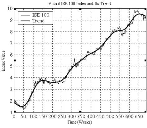
The trend and cyclical components of the weekly ISE 100 series are shown in Figure 3.4.1, with the trend obtained through the HP filter by taking λ as 128000. One can observe from this plot that there are different cycles with different frequencies and peak values, simultaneously fluctuating around the trend.

Figure 3.4.1 Natural logarithm of the weekly ISE 100 index and the trend series for

1988-2000.

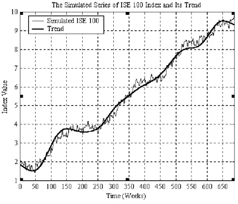
Figure 3.4.2 displays the simulated time series that corresponds to the weekly ISE 100 index. The trend component of the simulated series was taken to be the same as the trend of the actual series. Then, a major sinusoidal cycle with a period of 170 weeks and peak value of 0.25 was added upon this trend following Turhan-Sayan

21

Figure 3.4.2 The simulated weekly ISE 100 index and its trend component

and Sayan (2001). Next, 4 minor sinusoidal cycles with periods of 52 weeks (1 year), 26 weeks (6 months), 12 weeks (3 months) and 7 weeks were added and the sinusoidal peak values of minor cycles were chosen as 0.1, 0.1, 0.1, and 0.09, respectively, so that the cyclical component of actual ISE 100 index and cyclical component of simulated series would look similar. This corresponds to taking n as 5 and letting p1 = 0.25, T1 = 170 weeks, p2 = 0.1, T2 = 52 weeks, p3 = 0.1, T3 = 26

weeks, p4 = 0.1, T4 = 12 weeks, p5 = 0.09 and T5 = 7 weeks in terms of the notation

22

CHAPTER 4

THE RESULTS

This chapter compares the performance of HP and BP filters implemented on the simulated ISE 100 series with different parameter configurations in approximating the known trend and cyclical components.

4.1 The HP Filter Results

To filter the simulated ISE 100 index, the HP filter was used by assigning different values to λ , the smoothing parameter, including those suggested by Hodrick and Prescott (1997). The λ values considered were 10, 20, 30, 40, 50, 60, 70, 80, 90, 100, 400, 1600, 14400, 57600, 65000, 80000, 115200, 128000, 256000, 384000 and 512000. The trend components of the simulated series of weekly ISE 100 index values obtained by the HP filter using these λ values were then compared to the known trend component, obtained from the actual series with HP(128000)2 by using the error measurement criteria suggested before. Table 4.1.1 shows the results of the error measurements for each λ value.

2 _{In the rest of the discussion, HP(a number) is used to refer to the HP filter with λ value given in}

23

Table 4.1.1 The MSAE Values for the Trend Components of the Simulated ISE 100

Index Obtained by the HP Filter λ MSAE(%) 10 4.00 20 3.96 30 3.94 40 3.93 50 3.92 60 3.92 70 3.91 80 3.91 90 3.90 100 3.90 400 3.85 1600 3.81 14400 3.77 57600 3.82 65000 3.82 80000 3.83 115200 3.86 128000 3.87 256000 4.02 384000 4.16 512000 4.29

As can be seen from the table, the minimum error (3.77%) is given by HP(14400) filter. The numbers in the table indicate, perhaps more than anything else, that the errors on trend values are not that sensitive to the choice of λ value. For instance, the MSAE value for λ=10 (4.00%) is about the same as the MSAE value of λ=256000 (4.02%) although the difference between these λ values is huge. A similar observation applies to the trend series obtained by using the HP filter with λ values of 400 and 115200, since the MSAE values corresponding to these trend components (3.85% and 3.86%) are about the same (and pretty close to others reported in the table). Figure 4.1.1 shows the known trend series and the trend

24

series of the simulated weekly ISE 100 index obtained by using the HP filter with a λ value of 14400.

Figure 4.1.1 Comparison of trend components of simulated weekly ISE 100 index

obtained by the HP(14400) filter against the known trend series.

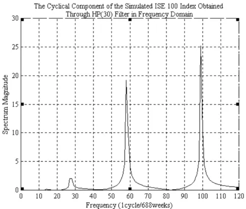
Although the HP(14400) filter showed the minimum error for the trend component, when the Fourier transformation of the corresponding cyclical component was analyzed as in Turhan-Sayan and Sayan (2001b), it was observed that the frequencies of the cycles with period lengths of 7 weeks, 12 weeks, 26 weeks and 52 weeks are differentiated easily, whereas the frequency of the major 170-week cycle is not clear. (A basic description of the Fourier transformation is given in the Appendix.) This leads one to think that the MSAE values for the trend components might not be explanatory about the performances of the HP filters with different λ values in capturing the business cycles present in the time series. Figure 4.1.2 shows

25

the frequency domain representation of the cyclical component of the simulated ISE 100 index obtained through the HP(14400) filter.

Figure 4.1.2 Frequency domain representation of the cyclical component of

simulated weekly ISE 100 index obtained by the HP(14400) filter.

In this plot, the peak at x=14 corresponds to the cycle with period length of 52.92 weeks by the following relationship:

f1=(14-1)/688=13/688 cycles/week, T1=1/f1=688/13=52.92 weeks (vs. 52 weeks) where f1 is the frequency and T1 is the period of the cycle. Similarly, the peak at x=27 shows a cycle with a period length of 26.46 weeks (vs. 26 weeks). The peaks at x=58 and x=99 denotes cycles with period lengths of 12.07 weeks (vs. 12 weeks) and 7.02 weeks (7 weeks), respectively.

26

As for the errors for cyclical components obtained through the HP filter with different λ values, Table 4.1.2 shows the MSAE value for each λ.

Table 4.1.2 The MSAE Values for the Cyclical Components of the Simulated ISE

100 Index Obtained by the HP Filter λ MSAE(%) 10 231.16 20 222.92 30 216.35 40 219.04 50 220.61 60 221.76 70 232.48 80 242.20 90 250.77 100 258.62 400 377.90 1600 476.41 14400 580.43 57600 651.46 65000 657.94 80000 669.10 115200 688.84 128000 694.58 256000 729.83 384000 749.66 512000 763.39

The results in this table indicate that, unlike the case with trend components, error measurements for the cyclical components are highly sensitive to the choice of λ. Increasing the value of λ beyond 30 results in significant increases in errors particularly after λ=100. Although for λ values of 10 and 256000 the MSAEs for trend components are the same, this is not the case for the cyclical components. There is a big gap between MSAE values of λ=10 (231.16%) and λ=256000 (729.83%). Similarly, MSAE values for the cyclical components obtained by using

27

λ values of 400 and 115200 are far apart with the MSAE value for λ=400 being 377.90%, whereas the MSAE value for λ=115200 is 688.84%.

This implies that the choice of λ values should depend on MSAE values for cyclical components rather than those for trend components. Given that the minimum MSAE value for the cyclical component is obtained at λ=30, the results appear to point to a low λ value.

It is also worth noting that the variation between the MSAE values for trend and cyclical components is very high. For instance, the MSAE value for the trend component obtained through the HP(30) filter is 3.94%, while the MSAE value for the corresponding cyclical component is 216.35%. The reason behind this difference is that there exist outliers in the absolute errors calculated for the cyclical components. An outlier refers to a data point with an absolute error value of greater than one standard deviation of the absolute errors of the whole sample. For the λ value of 30, the number of outliers, i.e., the sample points with absolute errors greater than 9.04, is 21. When absolute errors of these points are subtracted from the total absolute errors of the sample, the MSAE value decreases to 111.09%.

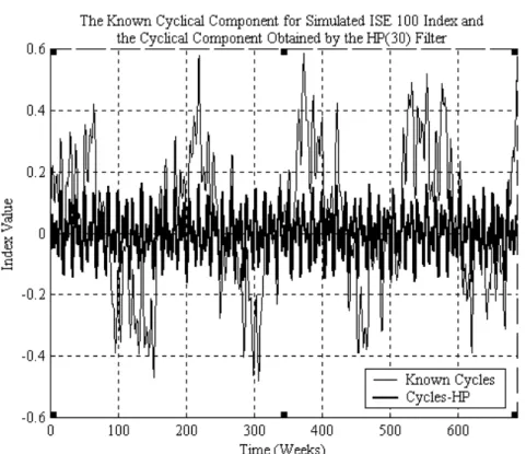
Figure 4.1.3 shows the known cycles and the cyclical component of the simulated weekly ISE 100 index obtained by using the HP filter with λ 30. Since most of the cyclicality is included in the trend series, cyclical component of the simulated series obtained through HP(30) cannot catch the long cycles, even though they are known to be present.

28

Figure 4.1.3 Comparison of cyclical components of simulated weekly ISE 100

index obtained by the HP(30) filter against the known cycles.

The cyclical components obtained through the HP filter with different λ values were analyzed using the Fourier transforms. An examination of these frequency domain representations shows that not all frequencies corresponding to the cycle lengths of the cyclical component of the simulated series can be observed. Figure 4.1.4 shows the frequency domain representation of the cyclical component of the simulated series obtained by using the HP filter with λ 30.

29

Figure 4.1.4 Frequency domain representation of the cyclical component of

simulated weekly ISE 100 index obtained by the HP(30) filter.

From this plot, cycles with period lengths of 7.02 and 12.07 weeks (the cycles that correspond to the peaks at x=99 and x=58, respectively) can be easily differentiated, whereas the cycles of 170 weeks and 52 weeks are not visible. The 26.46 week-cycle brings about a peak with a little spectrum magnitude at x=27.

Although the MSAE value for the cyclical component obtained through the HP(30) filter displayed the minimum value, it could not identify all the cycles existing in the cyclical component of the simulated series of the ISE 100 index, when the frequency content of the cyclical component was analyzed. This signals that the MSAE values for the cyclical components might not be reliable for the performance comparison of different λ values of the HP filter.

30

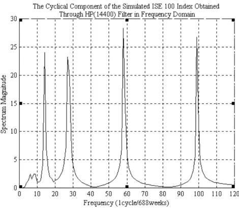
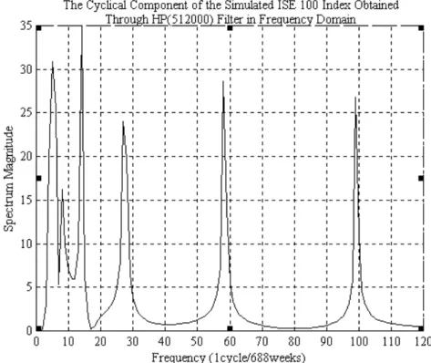
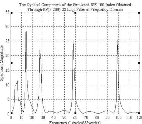
On the other hand, when the Fourier transforms of the cyclical components obtained through the HP filter with λ values greater than 14400 are analyzed, the frequencies of all cycles existing in the cyclical component of the simulated series can be distinguished. The magnitude of the peak of the frequency that corresponds to the cycle length of 170 weeks increases as λ increases. Nonetheless, the HP filter with λ values greater than 14400 creates one more cycle, in addition to the existing ones, in the cyclical component of the simulated series as shown in Figure 4.1.5. This figure displays the Fourier transform of the cyclical component of the simulated ISE 100 index obtained by using the HP(512000) filter. The reason for selecting 512000 as the λ value is that the frequencies of the cycles existing in the cyclical component of the simulated series are best visible for this λ value.

Figure 4.1.5 Frequency domain representation of the cyclical component of

31 According to Figure 4.1.5, the peak at

x=5 shows a cycle with f1=(5-1)/688=4/688 cycles/week, T1=1/f1=688/4=172 weeks (vs. 170 weeks representing an error of 1.18%),

x=14 shows a cycle with f2=(14-1)/688=13/688 cycles/week, T2=1/f2= 688/13=52.92 weeks (vs. 52 weeks representing an error of 1.77%)

x=27 shows a cycle with f3=(27-1)/688=26/688 cycles/week, T3=1/f3= 688/26=26.46 weeks (vs. 26 weeks representing an error of 1.77%)

x=58 shows a cycle with f4=(58-1)/688=57/688 cycles/week, T4=1/f4= 688/57=12.07 weeks (vs. 12 weeks representing an error of 0.58%)

x=99 shows a cycle with f5=(99-1)/688=98/688 cycles/week, T5=1/f5= 688/98=7.02 weeks (vs. 7 weeks representing an error of 0.29%)

x=8 shows a (spurious) cycle with f6=(8-1)/688=7/688 cycles/week, T6=1/ f6=688/7=98.28 weeks

where f is the frequency and T is the period length of the cycle. The frequency responses of peaks that are related to the peak values of cycles (the parameter a used during the construction of the cyclical component) were also the best approximations for the frequency responses of the cycles existing in the known cyclical component.

Yet, this plot points to one more frequency, corresponding to 98.28 weeks, even though it was not imposed upon the known trend series during the construction of the simulated series. This finding is in parallel to findings of Harvey and Jaeger (1993), and Cogley and Nason (1995) who argued that the HP filter might result in spurious cycles which are not present in the original data. It should be noted that the

32

HP filter with λ values below 512000 could also detect the business cycles, though with lower intensities. This means that the frequency response of the spurious cycle would also be lower. However, if the main concern is to detect the business cycles with the right frequency responses, then the usage of HP(512000) filter is acceptable even though it yields a spurious cycle.

It can be concluded in general that the MSAE measurements of the trend components of the simulated series obtained by using the HP filter are not sensitive to the choice of λ. However, the MSAE measurements of the cyclical components of the simulated series obtained by using the HP filter give highly distinct responses to changing λ values. The minimum error for the cyclical component is reached when the HP filter is used with λ value of 30. For the frequency domain representations of the cyclical components of the simulated series, the best performance (in terms of the observability of the exact frequency values of the cycles existing in the known cyclical component) is achieved by HP(512000).

4.2 The BP Filter Results

The BP filter has three parameters: lengths of the shortest and longest periods for the cycles and the number of lags, K. For this reason, various combinations of these parameters were tried, while running the BP filter algorithm.

33

Firstly, the trend component of the simulated weekly ISE 100 index was obtained, when the shortest period length was 3 weeks and the longest period length was 180 weeks which include the shortest and longest cycle length values (7 weeks and 170 weeks, respectively) used in simulating the actual weekly ISE 100 index. These two period lengths were processed with 7 different lag values: 12, 20, 28, 36, 44, 52 and 60. The filtering process was started with the lag number of 12, the lowest lag value suggested by Baxter and King (1999) for the BP filter in the analysis of quarterly data, and the effect of increasing the number of lags to accommodate weekly data was investigated.

Alternative lengths of 200 and 250 weeks were also tried as the maximum cycle length, while retaining the number of lags. Since the trend component of a series could be viewed as the low-frequency component of the series, changes in the lowest period length (3 weeks) do not affect the resulting trend component. Thus, the lowest period length, i.e., the highest frequency component of the filter, was not changed in repeated applications of the BP filter to the simulated series of weekly ISE 100 index. Table 4.2.1 shows the comparative error measurement results with the known trend series and the trend component of the simulated weekly ISE 100 index obtained by using BP filter under alternative parameter configurations.

As in the case of the HP filter, MSAE value for the trend component is not sensitive to the choice of the largest period length and the lag number, K. The error terms are fluctuating between 3.69% and 4.00%. The minimum MSAE measurement from the comparison of trend components is obtained with the largest period length of 180

34

Table 4.2.1 The MSAE Values for the Trend Components of the Simulated ISE 100

Index Obtained by the BP Filter

BP Filter MSAE (%) BP12 (3,180) 3.78 BP20 (3,180) 3.84 BP28 (3,180) 3.92 BP36 (3,180) 3.98 BP44 (3,180) 3.92 BP52 (3,180) 3.82 BP60 (3,180) 3.69 BP12 (3,200) 3.78 BP20 (3,200) 3.84 BP28 (3,200) 3.92 BP36 (3,200) 3.99 BP44 (3,200) 3.94 BP52 (3,200) 3.85 BP60 (3,200) 3.74 BP12 (3,250) 3.78 BP20 (3,250) 3.84 BP28 (3,250) 3.93 BP36 (3,250) 4.00 BP44 (3,250) 3.96 BP52 (3,250) 3.89 BP60 (3,250) 3.82

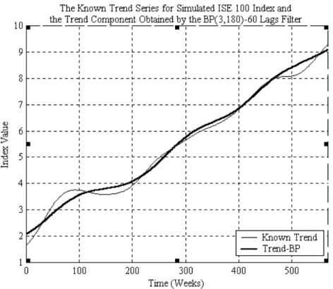
and the lag number of 60 (3.69%). Although the difference between the MSAE measurements of BP60 (3,180) (3.69%) and BP12 (3,180) (3.78%) is not marked (0.09%), the loss of 96 data points from the sample is not tolerable for this amount of error reduction. Thus, the results in Table 4.2.1 do not allow for a strong conclusion to be drawn about the performances of the filters with respect to error measurement values for the trend components of the simulated series. Figure 4.2.1 shows the known trend series and the trend series of the simulated weekly ISE 100 index obtained by using the BP60 (3,180) filter. Since 120 data points are lost (60 from the beginning, 60 from the end of the sample), the figure includes the remaining 568 data points.

35

When the frequency domain representation of the corresponding cyclical component was analyzed, it was observed that all cycles that are known to exist in

Figure 4.2.1 Comparison of trend components of simulated weekly ISE 100 index

obtained by the BP60 (3,180) filter against the known trend series.

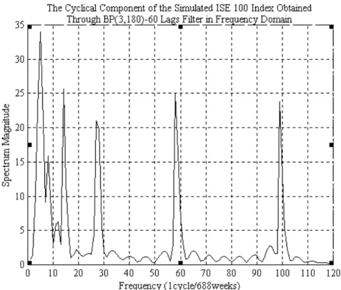
the simulated series of the ISE 100 index were identified by using the BP60 (3,180) filter. Figure 4.2.2 shows the frequency domain representation of the cyclical component of the simulated ISE 100 index obtained by using the BP60(3,180) filter.

The cycles present in the cyclical component are identified as follows: Peak at x=5 refers to T=688/(5-1)=172 weeks (vs. 170 weeks)

Peak at x=14 refers to T=688/(14-1)=52.92 weeks (vs. 52 weeks) Peak at x=27 refers to T=688/(27-1)=26.46 weeks (vs. 26 weeks) Peak at x=58 refers to T=688/(58-1)=12.07 weeks (vs. 12 weeks)

36

Figure 4.2.2 Frequency domain representation of the cyclical component of

simulated weekly ISE 100 index obtained by the BP60(3,180) filter.

Peak at x=99 refers to T=688/(99-1)=7.02 weeks (vs. 7 weeks) Peak at x=8 refers to T=688/(8-1)=98.29 weeks (spurious cycle) Peak at x=12 refers to T=688/(12-1)=62.55 weeks (spurious cycle)

with the rest of the movements representing noisy cycles. Although the BP60(3,180) filter showed the minimum error for the trend component, the corresponding cyclical component has two significant spurious cycles and a number of noisy cycles in addition to the ones imposed during the construction of the simulated series. Hence, it can be concluded that the filter with minimum MSAE value might not exactly correspond to the cyclical component made up of only the true cycles.

37

Table 4.2.2 shows the MSAE values for cyclical components obtained through BP filter with different cycle lengths and lag number parameters. The results in this table reveal that error measurement values of the cyclical components are highly sensitive to the changes in the lag parameter and the length of the largest period. Increasing the number of lags increases the MSAE value. BP12 (3,180) filter displays the minimum error value of 518.57%.

Table 4.2.2 The MSAE Values for the Cyclical Components of the Simulated ISE

100 Index Obtained by the BP Filter

BP Filter MSAE (%) BP12 (3,180) 518.57 BP20 (3,180) 723.97 BP28 (3,180) 677.02 BP36 (3,180) 774.62 BP44 (3,180) 878.11 BP52 (3,180) 870.99 BP60 (3,180) 864.60 BP12 (3,200) 518.66 BP20 (3,200) 724.77 BP28 (3,200) 677.43 BP36 (3,200) 777.23 BP44 (3,200) 886.61 BP52 (3,200) 878.97 BP60 (3,200) 883.72 BP12 (3,250) 518.78 BP20 (3,250) 725.83 BP28 (3,250) 677.97 BP36 (3,250) 780.77 BP44 (3,250) 898.29 BP52 (3,250) 892.88 BP60 (3,250) 910.99

Again, the gap between the MSAE values of the trend components and the cyclical series is very large. This is due, to some extent, to the outliers (i.e., data points for which absolute error is greater than one standard deviation of the absolute errors of

38

the whole sample) that exist in the cyclical component of the simulated series extracted by using the BP filter. For the cyclical component of the simulated ISE 100 series, there are 8 outliers for which absolute errors are greater than 43.65. When the total absolute errors of outliers are dropped from the sample, the error measurement value of the cyclical component of the simulated series obtained by using BP12 (3,180) decreases to 166.81%. Figure 4.2.3 shows the known cycles and the cyclical component of the simulated weekly ISE 100 index obtained by using BP12 (3,180). Due to the use of 12 lags, 24 sample points are lost and the figure displays 664 data points.

Figure 4.2.3 Comparison of cyclical components of simulated weekly ISE 100

index obtained by the BP12 (3,180) filter against the known cycles.

Given that error measurement values of the trend components are not sensitive to the choice of parameters, whereas those of the cyclical components are highly

39

responsive to the choice of the lag number, a certain conclusion about the reliability of the BP filter with different parameters cannot be drawn. This leads one to investigate the Fourier transforms of the cyclical components of the simulated series obtained through the BP filter with different cycle lengths and lag numbers.

An examination of the frequency domain representations of the cyclical components of the simulated series of weekly ISE 100 index obtained by the BP filter shows that all filters catch the cycles with the period lengths of 7 weeks, 12 weeks, 26 weeks and 52 weeks. However, as in the case for the HP filter, although the BP12 (3,180) filter showed the minimum MSAE value for the cyclical component, it could not identify all the cycles present in the simulated series of the ISE 100 index. This, again, gives rise to unreliability of the MSAE values measured for the cyclical components. In order to help visualize this, Figure 4.2.4 shows the frequency content of the cyclical component of the simulated ISE 100 index obtained through the BP12 (3,180) filter.

The frequencies of the cycles with 7, 12, 26 and 52 weeks (i.e., the peaks at x=99, x=58, x=27 and x=14, respectively) can easily be observed in this figure but the one with 170 weeks does not show up. Although the longest period length does not matter, the lag number makes a difference for the identification of the major

40

Figure 4.2.4 Frequency domain representation of the cyclical component of

simulated weekly ISE 100 index obtained by the BP12 (3,180) filter.

business cycle. When the Fourier transforms of the cyclical components of the simulated series extracted through the BP filter with lag numbers greater than 28 are considered, on the other hand, frequencies of all business cycles including the major one become observable. Nevertheless, the BP filters with lag numbers of 36, 44, 52 and 60 do exhibit one more cycle with a period length of 98.29 weeks. This implies that although higher lag numbers result in higher frequency response of the 170 weeks cycle, it also causes frequency response of the spurious cycle to be more noticeable. Since the length of the longest cycle period does not make any difference for the identification of the cycles, the BP filter with longest cycle length of 200 weeks can be picked to show the performance of the filter with 28 lags. (The use of BP28 (3,200) filter requires losing 56 data points from the sample, which appears tolerable. This is another reason for selecting the BP28 (3,200) filter as the

41

one with the best performance.) Figure 4.2.5 displays the Fourier transform of the cyclical component of the simulated ISE 100 index obtained by using BP28 (3,200) filter.

Figure 4.2.5 Frequency domain representation of the cyclical component of

simulated weekly ISE 100 index obtained by the BP28 (3,200) filter.

This plot makes it possible to differentiate frequencies of all cycles that are sought. The peak at x=5 shows the existence of a cycle with 172 weeks period length. Similarly, the peaks at x=14, x=27, x=58 and x=59 stand for cycles with period lengths of 52.92, 26.46, 12.07 and 7.02 weeks respectively. The frequency response of the 170 week-cycle is the minimum although it was the major cycle. This value increases with increasing number of lags, and since high values of lags introduce a spurious cycle with period length of 98.29 weeks, using 28 lags for the BP filter is appropriate. On the other hand, if the aim is also to approximate the magnitude of

42

the peaks (indicated by the coefficients of cycles imposed), use of high lag numbers could be justified - although this might cause undesirable cycles to be introduced.

In conclusion, the error measurements of trend components of the simulated series obtained through the BP filter are not sensitive to the changes in the values of filter parameters. But the opposite is true for the MSAE values of the cyclical components of the simulated series extracted by using the BP filter. Small changes in the lag numbers bring about great differences in the error measurement values of the cyclical components. Considering the frequency domain representations, the best performance in catching the exact cycles sought is obtained using the BP filter with 28 lags.

4.3 Application to Actual Data

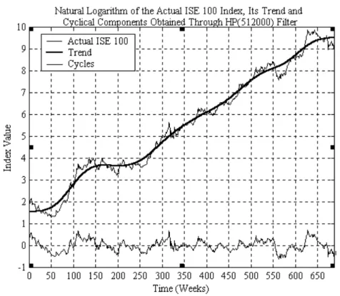
The HP filter showed the best performance when λ value was set to be 512000. This filter was also applied to the actual weekly ISE 100 index. Figure 4.3.1 shows the actual index, its trend and cyclical components obtained through the HP(512000) filter.

43

Figure 4.3.1 Natural logarithm of the actual ISE 100 index and its trend and

cyclical components obtained by using the HP(512000) filter.

To see the period lengths of the cycles existing in the cyclical component, the frequency domain representation of the cyclical component was also examined. Figure 4.3.2 shows the resulting plot.

The analysis of the figure leads to the following conclusions: There are mainly 5 peaks that can be identified easily. The peak at

x=5, T=688/(5-1)=172 weeks (vs. 172 weeks which was observed in the cyclical component of the simulated ISE 100 index obtained through the HP(512000) filter) x=8, T=688/(8-1)=98.29 weeks (vs. 98.29 weeks which was observed in the cyclical component of the simulated ISE 100 index obtained through the HP(512000) filter as a spurious cycle)

44

Figure 4.3.2 The frequency domain representation of the cyclical component of the

actual ISE 100 index obtained by using the HP(512000) filter

x=14, T=688/(14-1)=52.92 weeks (vs. 52.92 weeks which was observed in the cyclical component of the simulated ISE 100 index obtained through the HP(512000) filter)

x=19, T=688/(19-1)=38.22 weeks x=21, T=688/(21-1)=34.4 weeks

Also, the peaks at x=28 and x=57 correspond to cycles with respective period lengths of 25.48 and 12.29 weeks which were the cycles used during the construction of the simulated series of the ISE 100 index.

Similarly, the BP28 (3,200) filter was applied to the actual ISE 100 index, yielding the trend and cyclical components that are shown in Figure 4.3.3.

45

Figure 4.3.3 The natural logarithm of the actual ISE 100 index and its trend and

cyclical components obtained by using the BP28 (3,200) filter.

Due to the loss of 56 sample points resulting from the use of 28 lags, the figure consists of 632 data points. As it was done for the HP filter, the frequency domain representation of the cyclical component was analyzed. The frequencies of the cycles obtained from BP filtering are shown in Figure 4.3.4.

When this plot is investigated, it is observed that there are 5 main cycles with the following peak values:

x=5, T=688/(5-1)=172 weeks (vs. 170 weeks, the period length of the major cycle used during the construction of the simulated ISE 100 index)

x=9, T=688/(9-1)=86 weeks

x=14, T=688/(14-1)=52.92 weeks (vs. 52 weeks, the period length of the minor cycle used during the construction of the simulated ISE 100 index)

46

Figure 4.3.4 The frequency domain representation of the cyclical component of the

actual ISE 100 index obtained through the BP28 (3,200) filter.

x=18, T=688/(18-1)=40.47 weeks

x=21, T=688/(21-1)=34.4 weeks (this cycle was also identified by using the HP(512000) filter).

47

CHAPTER 5

ROBUSTNESS OF THE RESULTS

In order to test the robustness of the results, another series was constructed to simulate the behavior of weekly Jasdaq index. The Jasdaq index was used to see whether the conclusions drawn from the application of the HP and BP filters to the simulated series of ISE 100 index would remain applicable for a series whose volatility (standard deviation) is much lower than the actual ISE 100 index (standard deviation of actual ISE 100 index is 2.46 whereas standard deviation of actual Jasdaq index is 0.34).

5.1 The Data

The actual Jasdaq index consists of 470 sample points (Friday closing values) over the period from January 3, 1992 to December 29, 2000. The trend of the actual Jasdaq index was obtained through the HP(128000) filter and was used as the trend component of the simulated series. Figure 5.1.1 shows the actual Jasdaq index and the trend series.

48

Figure 5.1.1 Natural logarithm of the weekly Jasdaq index and the trend series for

1992-2000.

To construct the cyclical component of the simulated series, 4 sinusoidal cycles were used by taking p1=0.12, T1=160 weeks; p2=0.085, T2=100 weeks; p3=0.06,

T3=30 weeks; p4=0.04 and T4=6 weeks, as mentioned in Section 3.3. Then, by

imposing this known cyclical component over the known trend series, the simulated series of Jasdaq index was constructed. Figure 5.1.2 shows the simulated series of Jasdaq index and its trend.

49

Figure 5.1.2 The simulated weekly Jasdaq index and its trend component.

5.2 The HP Filter Results

The same procedure used in creating the series that simulates the ISE 100 index was applied to construct the series simulating Jasdaq index. First, the constructed series was filtered through the HP filter with different λ values. The trend components obtained were compared to the known trend series considering the sum of absolute errors (MSAE) criteria. The resulting error measurements are shown in Table 5.2.1.

Similarly to the trend component of simulated series of the ISE 100 index, the MSAE values are not so responsive to the changes in λ value. The same error value

50

Table 5.2.1 The MSAE Values for the Trend Components of the Simulated Jasdaq

Index Obtained by the HP Filter λ MSAE(%) 10 2.31 20 2.30 30 2.30 40 2.29 50 2.29 60 2.28 70 2.28 80 2.27 90 2.27 100 2.26 400 2.20 1600 2.14 14400 2.10 57600 2.12 65000 2.13 80000 2.14 115200 2.18 128000 2.19 256000 2.33 384000 2.44 512000 2.52

(2.20%) was reached both for the HP(400) and HP(128000) filters, for example, although the second λ value is 320 times greater than the first one. Figure 5.2.1 shows the known trend series and the trend component of the simulated Jasdaq index obtained through the HP(14400) filter (since the minimum MSAE value of 2.10% was obtained by using this filter).

In order to examine the frequency content of the corresponding cyclical component obtained by using the HP(14400) filter, the frequency domain representation of the

51

Figure 5.2.1 The known trend series and the trend component of the simulated

Jasdaq index obtained through the HP(14400) filter.

known cyclical component was analyzed. Figure 5.2.2 shows the frequencies for the cycles of the known cyclical component of the simulated Jasdaq index.

This plot clearly shows the frequencies of the business cycles used to construct the known cyclical series. As described in the Appendix, the peak at x=4 shows a cycle with a period length of 156.67 weeks (vs. 160 weeks representing an error of only 2.08%). The formula used to find the period length of the cycle is as follows:

52

Figure 5.2.2 The frequency domain representation of the known cyclical

component of the simulated Jasdaq Index.

f1=(4-1)/470=3/470 cycles/week, T1=1/ f1=470/3=156.67 weeks where f1 is the frequency of the cycle and T1 is the period length of the cycle. Similarly, the peak observed at x=6 stands for another cycle of 94 weeks length (vs. 100 weeks with an error of 4%). The other peaks at x=17 and x=79 are for cycles with period lengths of 29.38 weeks (vs. 30 weeks with an error of 2.07%) and 6.03 weeks (vs. 6 weeks with an error of 0.5%), respectively. The frequency responses of these peaks are in correspondence with the sinusoidal peak values of the business cycles imposed over the known trend during the construction of the simulated series of the Jasdaq index. For instance, the ratio between the coefficients of the 160 weeks and 6 weeks cycle (p1/p4=0.12/0.04=3) is preserved for the ratio between the frequency responses of

53

x=4 is 24, the frequency response of the peak at x=79 is 8 and 24/8=3 is the same as

p1/p4 value).

The frequency content of the cyclical component of the simulated Jasdaq index obtained through the HP(14400) filter is in Figure 5.2.3.

Figure 5.2.3 Frequency domain representation of the cyclical component of

simulated weekly Jasdaq index obtained by the HP(14400) filter.

In this plot, the peaks at x=6, x=17 and x=79 refer to the business cycles with period lengths of 94, 29.38 and 6.03 weeks respectively. As in the case of the simulated ISE 100 index, the cyclical component that corresponds to the HP(14400) filter displaying the minimum MSAE value for the trend does not include the major business cycle with a period length of 160 weeks.

54

When the cyclical components of the simulated Jasdaq index obtained through the HP filter with the same values of λ were considered, a picture similar to the case of cyclical components of the simulated ISE 100 index emerged indicating that the MSAE values were considerably sensitive to the choice of the value of λ. The higher the value of λ is, the higher the MSAE value for the cyclical component. Table 5.2.2 shows the MSAE values for the cyclical components obtained through the HP filter with changing λ values.

Table 5.2.2 The MSAE Values for the Cyclical Components of the Simulated

Jasdaq Index Obtained by the HP Filter λ MSAE(%) 10 191.73 20 197.44 30 199.94 40 201.56 50 202.82 60 203.87 70 204.81 80 205.74 90 206.63 100 207.50 400 224.59 1600 250.44 14400 283.20 57600 311.94 65000 315.52 80000 327.91 115200 352.49 128000 360.19 256000 415.93 384000 451.22 512000 476.13

The results in the table point to conclusions similar to those previously derived about the cyclical components of the simulated series of the ISE 100 index. The

55

lower the value of λ, the lower the MSAE for the cyclical component with the minimum being reached at λ=10. Given the same MSAE value for the trend components obtained through the HP(400) and HP(128000) filters, the MSAE values obtained for the corresponding cyclical components are remarkably different, 224.59% for HP(400) versus 360.19% for HP(128000). A similar observation could be made for the error measurements of the cyclical components obtained through the HP(10) and HP(256000) filters. In both cases, the lower value of λ corresponds to a lower MSAE value for the cyclical component of the simulated Jasdaq index. Figure 5.2.4 shows the known cyclical component and the one obtained by using the HP(10) filter for which the MSAE is at its lowest value (191.73%).

Figure 5.2.4 The cyclical component of the simulated Jasdaq index obtained