ISTANBUL UNIVERSITY -
JOURNAL OF ELECTRICAL & ELECTRONICS ENGINEERING YEAR VOLUME NUMBER : 2003 : 3 : 1 (745-758) Received Date : 30.10.2002
COMPARATIVE ANALYSIS OF KOLMOGOROV ANN AND
PROCESS CHARACTERISTIC INPUT-OUTPUT MODES
Georgi M. DIMIROVSKI
1Yuanwei JING
21 Department of Computer Eng., Dogus University, 34722 – Kadikoy / Istanbul, Turkey, and Institute of ASE-FEE, SS Cyril and Methodius University, 1000 – Skopje, R. of Macedonia
2School of Information Sci. & Eng., Northeastern Univ., 110006 – Shenyang, P.R. of China 1E-mail: [email protected] 2E-mail: [email protected]
ABSTRACT
In the past decades, representation models of dynamical processes have been developed via both traditional math-analytical and less traditional computational-intelligence approaches. This challenge to system sciences goes on because essentially involves the mathematical approximation theory. A comparison study based on cybernetic input-output view in the time domain on complex dynamical processes has been carried out. An analytical decomposition representation of complex multi-input-multi-output thermal processes is set relative to the neural-network approximation representations, and shown that theoretical background of both emanates from Kolmogorov’s theorem. The findings provided a new insight as well as highlighted the efficiency and robustness of fairly simple industrial digital controls, designed and implemented in the past, inherited from input-output decomposition model approximation employed.
Keywords: Approximation models, characteristic input-output modes, complex systems, infinite matrices, neural networks.
I. INTRODUCTION
It may seem a paradox, but all the exact science is dominated by the idea of approximation – Bertrand Russell
This outstanding statement by Russell, one of the two founders of modern mathematical science [50], best supports all endeavors of systems and control science in identification of approximate model representations of dynamical processes, no matter whether the word is about input-output black-box [47], [52] or structural state-space views [38], [53], and whether obtained by math-analytical [37], [38] or computational intelligence [49], [54], [55] methods. This
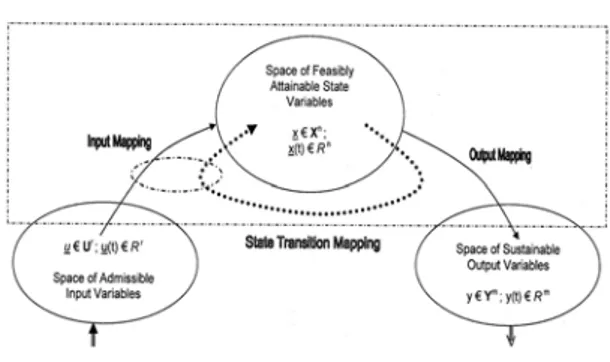
statement may well be readily inferred from Figure 1 on the fundamental concept of a dynamical system in engineering terms [9], [10]. For, indeed the word is about approximation
models for time-domain functions, functionals or
sequences that are theoretically consistent and empirically correct and valid.
By and large, all approaches to approximate system representations involve some kind of decomposition either from input-output or input-state-output points of view [10], [24]. The latter, of course, is associated intrinsically with the math-analytical fundamental approach [38], [53], and not with the one of the
computational-intelligence [49], [55]. the input-output (I/O) view the foundations of which were laid dawn by the founders of Cybernetics [47], [52]., however, generally applies to both of them to the same extent [17]. In addition, in both fundamental approaches the ideas of system decomposition and expansion have been exploited to the full, and both rely essentially on real-world recorded time series possessing all possible peculiarities [37], [41].
Fig. 1. The concept of a dynamical system in general, redefined in systems engineering terms according to essentially non-separable inter-play of fundamental natural quantities – energy, information, and matter – in dynamical processes.
In the present study, the focus is put on a comparative analysis [17] of certain approximate model representation results via math-analytical and neural-network techniques for the class of complex multi-input-multi-output (MIMO) processes having real-world natural steady-states such as in thermal plants [13]-[16]. Note, in addition, that certain on-site experiments were done before on real-world, high-power, industrial furnaces in addition to a number of experimental simulations [14]-[16], [45]. Here it is impossible, of course, to cite properly all the relevant references in the literature. Nonetheless, it is pointed out that some of them are found in the reference list included, and in the references therein. In particular, works based on the I//O systems view in the math-analytical (MAN) approach, [3], [5], [10]-[12], [21]-23], [29], and in the computational intelligence approach employing artificial neural networks (ANN), [1], [6], [19], [20], [27], [30], [31]-[36], [40], [43], [44], should be observed.
Next Section II gives a review discussion of some analytical results on I/O dynamical systems
representations via characteristic I/O modes decomposition [10], [11]-[13], [21]-[23]. Similarly, but in the realm of neural-network computing structures [2], [4], [26], [48], [51], some of the most outstanding representation results in the literature, are recalled as appropriate along with a relevant review discussion in Section III, where these are cited and referenced. In Section IV, the comparison findings are summarized. Conclusion, an appendix (on relevant tools from mathematical approximation theory) and references are given thereafter.
2. ON MATH-ANALYTICAL
BLACK-BOX IDENTIFIED
SYSTEM MODELS
Pragmatically, the main goal in real-world system engineering applications is always to drive the plant so as to achieve the desired state(s) out of the all attainable ones controlling by means of the specified task-oriented and set-point controls, i.e. by integrated control and supervision [1], [16]. For this purpose, firstly, a set of families of models is indispensable, at least for operating points at low-, medium-, normal- and maximum-operating loads. And, secondly, ultimately both control and supervision algorithms are implemented in terms of time-domain, discrete-time approximations of the theoretical designs as well as the practical stability of the overall system in all operating regimes must be ensured [14], [23], [45].
In this paper, the proper theoretical treatment of the process model identification, which is found elsewhere (e.g., see [24], [37], [38]), is left aside and reference is made to the typical practice of operating common industrial plants that have finite steady state equilibrium, as the case study of 25 MW reheating furnace RZS (see the schematic in Figure 2) in Skopje Steelworks [14], [16], [23] is. In principle, any identification and signal processing methods may be used. Then, for a complex
plant (N
out inpxN
N
i
inp =N number of inputs;
number of outputs) in a given plant environment
with specified operating conditions, systems engineering design starts with a designed identification experiment and a study of a family of steady-state, non-linear input/output
o
N
=
out
j i
y
models representing “energy/material supply
variables,
m
,to controlled measurable state variables, ” within respective ranges ofadmissible inputs and sustainable outputs; moreover, within ranges where these are convex. In addition, a set of empirically (by either observation or experiment) obtained impulse-response representations are made available.
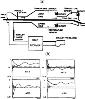
(a)
(b)
Fig. 2. Real-world 25 MW pusher furnace RZS illustrating this comparative study: the schematic (a) of and (b) the reduced errors via learning the process characteristic I/O modes for the identified kTSM model of main 2x2 sub-system ‘upper zone – lower zone’.
In here we make use of the case studies [14], [16], [45] of high-power, large, multi-zone, gas/oil-fired industrial furnaces (like the one in Fig. 2) where the main subset of measurable states are physical temperatures. The I/O approximation models that are operationally identified on the grounds of recorded non-linear time sequences [41] of input and output variables have the form
, ) , , ( j l i i i f m m const l j y T = = ≠ = o N i=1,..., , (1)
at the operating point
OpPo
, and µ µ µ=1,2,...,N[
]
[
]
T T t i o i oxN k NxNxN k t N kg
t
t
t
t
t
G
(
)
=
(
)
,
0≤
≤
(2a) or[
]
[
]
SS SS t i o i og
t
t
t
t
t
G
(
k)
NxN=
(
k)
NxNxN,
0≤
k≤
(2b) where truncation and steady-state time instants are finitet
T
t
< t
∞ andt
SS< t
∞. These modelsare produced by using admissible inputs with regard to the respective magnitude ranges at
operating point
µ
OpPo
µ
(a number of them).Ultimately, the latter two are in fact pseudo-impulse responses, discretized correctly with respect to the time, known as pseudo-weighting functions [3] or I/O weighting patterns [21], or as k-time sequence matrices [10], kTSM for short. In here, constant indicates the three-dimensional matrices of instantaneous values span up to the truncation time , and
t
is the time when steady state is reached, while theoretically T tN
Tt
SS +∞ → ∞t [10]. In any case, these are approximated three-dimensional infinite Markov matrices [29] of plant process dynamics that have been conveniently truncated. Note for thermal processes, having natural steady-states, these still can contain information on the local nonlinear distortions [10]-[13]. Hence identified models in all forms, relevant to the approach in the time domain, may readily be available:
[
]
T t i oxNxN N l kg
t
t
y
(
)
=
(
)
* ss k l lt
t
t
t
t
m
(
),
0≤
≤
<
(3) with * denoting convolution operation, and[
]
[
]
∞≅
t i o T t i oxNxN k N xNxN N lg
t
t
g
(
)
(
)
(3a) if only and if[
]
{
}
= → o i tT T N xN xN N l t t g N N ( ) 0 lim[
]
{
}
1 0)
(
lim
+→
o i tT T N xN xN N l tt
g
N
N
SS T t t N N → when ; (3b)[
(
)
]
(
)
[ ]
(
)
)
(
1 1 1 k xN N xN Nm
q
e
t
q
G
q
y
o o i o+
Ψ
=
− − − ; (4)[
]
[
]
[ ]
( )[ ]
( ); ) ( ), 1 ( ) ( ) 1 ( ) ( ) ( k xN N k xn N k k nxN s k nxn s k t e t x C t y t m T B t x T A t x o o o i Ψ + = − + − = (5)),
(
...,
),
1
(
(
)
(
t
kf
y
t
ky
t
kN
yy
=
−
−
.
),
1
(
t
k−
m
.)
(
))
(
...
),
1
(
),
(
.,
m
t
k−
t
λ−
N
me
t
k−
e
t
k−
N
e+
e
t
k (6)where and is the
vector of a zero-mean disturbance term. Of course, by allowing correctly for limited bandwidth via proper time sampling and using anti-aliasing filters, this enables always a convenient use of digital computations.
H
ence, the following formal definitions of characteristic I/O modes and vectors in the time domain for MIMO dynamical processes result [10], [21].o
]
) u y N N N R R f + → :e
(
t
k)
Definition II.1. The scalar Toeplitz operator
[
λ
i(tk is a characteristic input-output mode orpattern (CPA) of a MxM matrix plant
convolution (pseudo-impulse response) operator
[
G(tk)]
NoxNi =[
]
T t i oxNxN N kt
g
(
)
=ˆ
G
for,
M Nout = Ninp =t
0≤
t
k≤
t
∞,
[
]
if it is a root of the characteristic polynomial equation[
i(t )k I − G(tk) MxMxNtSS]
det
λ
. The Mx1 vectoroperator is a characteristic vector (CVE) if it satisfies the equation
)
(t
w
k{
λ
i(
t
k)
I
−
[
G
(
t
k)
]
MxMxN}w
(
t
k)
=
0
. (7) Apparently, the above concepts of CPA and the CVE describe the natural operationalinput-output dynamic behavior of plant convolution
operator
G
. In turn, plant convolution operator can be obtained by means of the spectral decompositionG
V
Λ
[
G
(
t
k)
]
MxMxN=
∑
iM=1λ
i(
t
k)
w
i(
t
k)
v
i(
t
k)
(8a) for simplicityW
G
=:
Λ
. (8b) Here, is a diagonal matrix comprising)
(
ki
t
λ
, which represent the CPA’s, and the columns ofW
=
V
−1=
[
w1 w2 ... wM]
i
are the CVE’s. The validity of the approximation can be confirmed by the known Gershgorin eigenvalue theorem for diagonal dominance. A normalization of the CVE is carried out such that each diagonal element of W is the identity element (1, 0, 0, ...), and also an reordering procedure using the decomposition result in [13] is carried out such that to each {
λ
} corresponds a constituent matrix with maximum norm on the diagonal element ‘i’ of approximated plant convolution operatorG
. iC
.
Gu
<
G
u
∞G
1.
Recall now that for any compatible set of norms there exists a vector norm (of signal variables), denoted by , of such that . Then
G
1,G
2, are system operator norms induced by signal norms ,.
2,.
∞, respectively. Operator elements of the kind of , together with the zeroO
and the identityG
I
operators, belong to a commutative Banachalgebra in which the product corresponds to discrete convolution [8] and may thus be manipulated using block-diagram algebra. The relationship between defined sequences and the corresponding stable or unstable Z-transforms is detailed by Cheng and Desoer in [5], who showed that the discrete time case can be treated by more straightforward methods in contrast to the continuous-time distributed case, which normally is plagued by difficult fine points of analysis. In addition, for Lure-Postnikov class of non-linear systems that are time-discretized, a left-distributive algebra on extended Banach spaces of p-summable (p=1, 2,
∞
) sequences exists [10]. It is well-known that the elements ofG
do not reveal the useful information about the interaction behavior of the plant, while the spectral decomposition (7)-(8) does [3], [10], [21].In principle, a CPA and associated CVE may be real and distinct, confluent or ones of a complex pair, however, for the well-posed gas furnaces they are real and distinct. When a CPA is real then its steady-state gain (SSG) matrix
G
is also real, and thus a simple test is to check thess
ss
eigenvalues of
G
. The CPA may be positive or negative, depending on the sign of its SSG; again, a simple test is to check the eigenvalues of . AG
has a characteristic inverse response pattern if a CPA is positive but the initial transient is negative, and vice versa, which implies that an eigenvalue of the first non-singular Markov matrixG
shall be positive if the eigenvalue of is positive. The CPA type is defined in the usual way for scalar operators, i.e. if the system type is the same for all elements along a row of then the CPA will take the same type. Internal process interaction is defined as the effect of one subsystem on the others, and this is reflected by the CVE precisely. If a CVE is aligned with its basis vector, i.e.G
)
(
t
k ssG
w
iG
I
=
, then is partially or triangular decoupled, and if all CVE are aligned with the basis vectors, i.e. , then is fully decoupled or non-interacting. If a CVE vary with timet
, the interaction is dynamic, otherwise it is static implying these vectors are zero for all . Static characteristic vectors imply that the constituents are constant real matrices.G
W
=
G
M
=
I
G
i NN
=
k kt
>
0
T tN
In real-world processes, the propagation information takes place along with flow and processing of energy and mass. Hence their behavior depend essentially on the magnitude of manipulated variables (which induces all sorts of nonlinear distortions that may be present in the plant), and hence the concept of energy and power balance within control loops has got a considerable impact [10], [17]. Moreover, from the energy balance point of view, the power contained in a kTSM operator of can be well-defined via a decomposition theorem [13]. For the purpose of the present comparative analysis its updated version [14] is stated below.
I/O Mode Decomposition Theorem II.1. The
ordered characteristic input-output modes of well-posed MIMO processes for
and , represented by three-dimensional k-time sequence matrices, have their natural decomposition in terms of characteristic signal power distribution
o N
N
N
=
(
)
∑
∑ ∑
= ==
==
M i i i i M i k M j jt
C
C
P
1 1λ
2(
)
1π
, (9a)∑
==
M i 1C
iI
, (9b)[
(
)
]
,
1 MxMxN kt
g
G
WLV
LV
V
−=
=
=
(10a),
T i i iw
v
C
=
(10b) with the constituent matrices Ci (CMA) of thecharacteristic I/O process modes
[
it
k]
NoxNixNL
=
λ
(
)
and characteristic vectors[
]
T xN N k ot
w
w
=
(
)
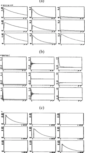
, which only in special cases may be constant.(a)
(b)
(c)
Fig. 2. Sample results for furnace RZS: (a) the identified pseudo-impulse response matrix; (b) the interaction characteristic vectors with time
i
characteristic modes extended with time delays. The set of constituent matrices, with their essential property (also see Figure 3 c), act as a modulating distributor of generalized power weights.
∑
==
M i 1
C
iI
It is apparent that the diagonal of reveals how generalized powers
i
C
π
are being associated with a particular diagonal element ofP
. In turn,P
may beobtained as a sum of convolutions between
π
i and , the arrayC
represents the power distribution weight in associated with the respective input-output process channel. Hence, the indicator of the proper position ofii l
C
ii l iiP
iλ
in the matrix structure is given by means ofMax{
∑
M==
i ii jC
1I
}, i = 1, 2,..., M, j =1,2,..., N. This indicator also represents the rule to
resolve characteristic I/O modes ordering and, consequently, the input-output pairing of controlling and controlled process variables. It is normally expected that the strongest interactions (represented by the elements of CVE and CMA) appear in the main diagonal of W. That is, a certain sub-system within MIMO systems ‘interacts mainly’ with itself validating the diagonal dominance in the process characteristic I/O modes has been attained. Figures 3 a, b, c for the real-world RZS pusher furnace provide a good physical illustration of the above presented I/O mode decomposition theorem as well as of the entire discussion in this section. Nonetheless, its is pointed out the word is about approximate representation models of operational processes in the plant object, where precisely the energy-information-matter inter-play goes on.
3. ON APPROXIMATION MODELS
BY ANN AND KOLMOGOROV’S
SECOND THEOREM
Within the context of artificial neural networks (ANN) in this paper, we are interested solely in approximation of functions applied to process model emulation identification. So, we confine
ourselves to a certain narrow area of approximation modelling of dynamical processes primarily using feed-forward ANN’s and solely to networks that emanate directly from Kolmogorov’s seminal results [31]-[32]. The emphasis is on Kolmogorov’s second theorem, which subsequently has been reformulated by Kurkova [34], [35] in more practical ways for ANN applications with somewhat relaxed requirements on approximating functions employed. This discussion follows the main streamline of mathematical theory of function approximation (for in depth study, see [33], [39], [42]) that is relevant for ANN based applications to generate approximate models, which represent stable but complex dynamical processes having natural steady-state equilibrium (e.g., industrial thermal systems) of interest in this comparative study. It should be noted, in addition, that computing ANN system structures are also readily modeled [2], [26], [51] by using theory of directed graphs [7], [25].
Now let here recall (6), which represents a fairly general input-output representation of time-discretized system models, where by assumption the underlying mapping
is continuous. In its very essence, the neural modeling approach makes use of ANNs for approximate representation of this function. Hence the neural modeling, in its very essence, is a problem of mathematical approximation theory. o u y N N N R R f + → :
Formal mathematical formulation of the problem of neural modeling using feedforward neural networks can be stated as follows. Consider a continuous mapping
where is an uncountable compact subset of o N C
R
S
f
:
→
S
C o NR
. Compactness of implies that it is closed and bounded, which is a realistic assumption given the fact that operating conditions are specified by means ofadmissible inputs and sustainable outputs, i.e.
represented by some bounded functions of time. Of course, the mapping is not given explicitly, but rather by a finite number of pairs
{
U
} CS
f
)
(
),
(
t
kY
t
k∈
S
CxR
No, ,now representing the number of observed
T t
N
...,
,
1
k
=
T tN
input-output pairs, namely,
U
= [)
(
t
k),
1
...,
),
1
(
t
k−
y
y
(
t
k−
N
y);
(
t
k−
o u+
N
1
x
N
o)
f
(
f
u
iN
N
(
S
C ]...,
)
yN
)
CS
)
(
t
kN
uu
−
f
S
f
T is anvector, and
Y
is an vector. Then, seek to find a representation of the mapping by means of known functions and a finite number of real parameters, such that the representation yields uniform approximation of it over set , which should be well-posed interpolation hyper-surface . Hence, in essence, this is an existence problem independent of the form in which the mappingmay be given, and therefore approximating known functions implies qualitative property such as continuity of the mapping . On the other hand, by its very essence, finding the interpolation of the continuum
intrinsically implies constructing it by a finite number of argument-value pairs, which may done by appropriate learning/training method and algorithms [2], [4], [26], [48], [51].
(
ox
N
)
(
)
(
t
k=
y
t
k Cf
In the Appendix, there are found further points of argument in terms of a brief outline of the known abstract mathematical schema, compiled from the literature, via which main theorems of mathematical approximation theory have been derived along with these theorems.
At this point, let briefly relate the discussion in this section to the one in Section II. It may well be noticed in the conceptual definition and the respective math-analytical description of process characteristic I/O modes via k-time sequence matrices, (7)-(8), that these are existent per-se because of the physical nature of the class of real-world plants considered. And, finding their constructive digital computation is dealt with in the associated decomposition theorem, (9)-(10), which is equivalent to learning/training in the neural modeling approach. So, for the time being, one can notice that indeed between these two I/O modeling approaches some kind of reminiscent relationship exists.
In order to proceed further, here we recall and place into proper perspective a subset of the main results involving Stone-Weierstrass [46]
and Kolmogorov’s second [32] theorems, and the polemical discussions related to the latter in [19], [20], [27], [30], [34]-[36], [40], [43], [44]. These two theorems constitute the fundamental toolbox of the approximation theory. The Stone-Weierstrass theorem has been identified in the literature as a prime candidate for establishing the property of the existence of approximation representation , employing ANN’s, of the continuous mapping
, and more detail is found in the appendix. In the sequel we focus on Kolmogorov’ second theorem and the related polemics. ) (SC f o N C R S f : →
It is well known that artificial neural networks, because of the biological inspiration and greater transparency of the analysis, do have layered structures. The sigmoidal model is described by
∑
= + = = Nj T ij Y ij ij i b U d i N y 1α
σ
( ), 1,...., , (11)where
α
ij,dij∈R, b are parameters, andU
o ixN N ij∈R)
(
t
kU
=
is the input vector, described at the beginning of this section. This representation equation possess the identity of that of an ANN having input layer, sigmoidal hidden layer, and linear output layer. Similarly the radial-basis-function model has the structure∑
= = = N j ij c m Y i g U i N y ij ij 1α
, ( ), 1,...., , (12)∑
= − = = N j ij c m ij ij Y i g U c m i N y ij ij 1α
, ( / ), 1,...., . (13) Of course, in both cases, respectively, it is necessary and sufficient to show that the set of all finite linear combinations of SG and RB functions constitute a non-vanishing algebra separating points on a compact . This has been done, but the same has been Gaussian-function networks only after introducing the additional requirement of convexity of .o ixN N C
⊂
R
S
o ixN N CR
S
⊂
On the grounds of Stone-Weirstarss theorem it has been found out that the use of both the SG and the RB functions is suitable for uniform approximation of an arbitrary continuous mapping, their interpolation properties,
]
,
however, are different; in a sense the RB functions, unlike the SG, are designed for interpolation. On the other hand, the issue on finding the best approximation remains much more involved. Nonetheless, the way deep into the existence problem has been highlighted when Kolmogorov’s second theorem, which already had a decisive impact on approximation theory [39], [43], has been brought into ANN prospective [27].
During a decade or so Kolmogorov’s theorem, resolving the representation of continuous functions defined on an n-dimensional cube by sums and superposition of continuous functions of one variable, has been one of the focuses attracting attention in the theory and applications of neural modeling approach. Hence the main result of Kolmogorov [32] as well as the subsequent reformulation by Kurkova [34], [35], who disproved the criticism by Girosi and Poggio [20] and verified its essential relevance for the neural modeling approach, are recalled next.
Theorem III.1 (Kolmogorov’s Second). Any
function continuous on the n-dimensional unit cube can be represented in the form
,
E
=
[
0
,
1
nE
(
)
∑
+∑
= = = 211 1 1,..., ) ( ) ( n i n j ij j i n x x x fψ
ϕ
, (14)where and
ϕ
ij are real continuous functions of one variable, and the functionsϕ
ij are independent of the given function while only the functionsf
i
ψ
are specific for the given function .i
ψ
Kolmogorov has made clear that on the grounds of this theorem it is possible to represent exactly every continuous function of many variables as a superposition of a finite number of continuous functions of one variable and of a single particular function of two variables, viz. addition. Considerably later, Lorentz [39] has proved a simplification of Kolmogorov’s theorem in which the functions
ψ
i may be replaced by only one functionψ
, and Sprecher [43] has shown that the functionsϕ
ij bywith and some monotonic
increasing functions j ij
φ
α
const
ij=
α
jφ
. Only in the eighties, Hecht-Nielsen [27] has reformulated Sprecher's version of Kolmogorov's representation theorem and applied to neural network modeling, and so did Funahashi, thus the use of ANN’s was made plausible entirely. More recently Lin and Unbehauen [36], Katsuura and Specher [30], Sprecher [44] made yet other realizations based on Kolmogorov’s second theorem.,
n ijα
ψ
Theorem III.2 (Heht-Nielsen form of Sprecher’s version). Any continuous function defined on the
n-dimensional cube can
be implemented exactly by a three-layered network having 2n+1 units in the hidden layer with transfer functions from the input to the hidden layer and
[ ]
0
,
1
,
=
E
where
E
jφ
from all of the hidden units to the output layer.
In their work Girosi and Poggio, [20], have pointed to the two drawbacks of this theorem:
are highly non-smooth, and j
ij
φ
α
on thespecific function are not representable in a parameterized form. In turn, Kurkova [34], [35] eliminated both these difficulties by using staircase-like functions of a sigmoidal type in a SG feedforward neural network. It is well known that highly non-smooth functions encountered in mathematics are mostly constructed as limits or sums of infinite series of smooth functions (see the Appendix). Kurikova showed that all of the single-variable functions in Kolmogorov’s theorem are limits of sequences of smooth functions when staircase-like functions of sigmoidal type are used in the neural network. In fact, this type of function has the property that it can approximate any continuous function on any closed interval with an arbitrary accuracy. Note that, in fact, these functions are directly employed in all discrete-time system representation models and kinds of digital computer generated controls [14], [16], [45].
f
j
φ
In the course of deriving her arguments, Kurkova also contributed an appropriate reformulation of Kolmogorov’s second theorem within the realm of artificial neural networks Hence, this reformulation of the celebrated Kolmogorov's representation theorem is presented next.
N
Theorem III.3 (Kolmogorov-Kurkova). Let
with ,
n
∈
n
≥
3
σ
:R→E be a sigmoidal function, be a function of class ,, and f ) n ) ( 0 En C ∈
f C0(E
ε
be a positive real number.Then there exist k and staircase-like functions N ∈ i
ψ
,ϕ
∈
S
(
σ
)
nE
ij nx
)
∈
...,
such that for every holds true
x ,
1x
= (
(
ϕ
)
ε
ψ
< −∑
k=∑
= i n j ij j i n x x x f( 1,..., ) 1 1 ( ) , (15) whereS
(
σ
)
is the set of all staircase-like functions of the form∑
= += kj i i i
SC x b x c
f σ( ) 1
α
σ
( ). (16)This theorem implies that any continuous function can be approximated arbitrarily well by a four-layer sigmoidal feedforward neural network. It should be noted that already has been established (albeit not by Kolmogorov arguments) that even three layers are sufficient for approximation of general continuous functions [6], [19]. In general, approximate implementation of
ψ
i does not guarantee an approximate implementation of the original the specific function [36], implying that the former mustbe exactly realized.f
Clearly, also there are limitations of the applicability of Kolmogorov's theorem to neural networks for approximation of mappings
. For instance, in applications, one has to answer the question whether an arbitrary given multivariate function can be represented by an approximate realization of the corresponding functions o i N C
R
S
f
:
→
ψ
of one variable. However, the efforts towards applying this theorem are fruitful and important, as some useful neural networks like the sigmoidal feedforward network are correctly and properly described by Kolmogorov's representation theorem [17]. Moreover, it is readily applicable to real-world complex plants such as industrial furnaces [15], [16]. And, so has been the case when applying CVE-CPA-CMA decomposition theorem that worked always for multi-zone furnaces [14]-[16], [23].4. A SUMMARY OF
COMPARATIVE FINDINGS
A closer comparison analysis of the essential substances presented in Sections II and III reveals fairly well the existent of similarities and distinctive differences between the respective input-output time-domain model representations [17]. The ones discussed in the previous section, the foundation of which is Kolmogorov’s theorem and which make use of ANNs (e.g., see [16], [17]), of course, are the more ‘general’ ones, because these are fully consistent with the mathematical approximation theory [33], [39], [42] precisely. These are learned form the I/O time sequences as they ere recorded during plant operation.
It should be noted, however, the kTSM representation model of characteristic I/O modes decomposition [10], [13] in Section II also are based on operational real-world I/O time sequences carrying on most essential features of the process [14]. This, in turn, sheds new light on the similarities and differences between both these approximation model representations. The main difference appears in the fact that Kolmogorov ANN do imply decomposition and generalization in the time domain, while I/O k-time sequences CVE-CPA-CMA imply solely decomposition [14], [17]. By referring more closely to characteristic I/O mode decomposition formulae, (9)-(10), and to Kurkova’s formulae of Komogorov’s representation theorem, (15)-(16), despite the considerable difference a common underlying background is evident. Although derived by means of different arguments – the former have also exploited the engineering physics – clearly both have been derived within the context of approximation theory of multivariate functions [17].
Now, let consider comparing (14) in the original Kolmogorov representation theorem and the approximation inequality (15) of Kurkova, which implies replacing the exact expression representation with an approximate one. Also, for a convenient parallel between neural-network approximation in this Section III and convolution approximation in Section II, and recall the earlier comparison setting for expressions (7)-(8) and (9)-(10). In turn, it may
f
well be seen that a noticeable reminiscence becomes quite apparent [17].
In the final consequence, from the points of view in the present discussion, it has become evident above that ultimately the characteristic I/O mode decomposition also has its support in the general validity of Kolmogorov’s theorem. And, this provides the explanation why fairly simple designs of PI partially-decoupling digital controls of industrial furnaces [14], [23], [45] turned out to work in robustness way and considerably better than initially expected.
5. CONCLUSION
In the literature, there have been developed system representation models via both math-analytical and computational-intelligence approaches. However, both essentially involve mathematical approximation theory. In this work, a comparison study of approximate representation models of a class of complex stable MIMO processes through the time domain input-output view of math-analytical time-sequence and of the artificial neural networks has been elaborated.
An analytical decomposition representation of complex MIMO dynamical processes having natural steady-state equilibrium (such as in thermal systems) has been set relative to the ANN approximation representations based on Kolmogorov’s theorem and comparison analysis carried out. The main findings resulting out of this study have been presented, which show that both emanate from the theoretical background of Kolmogorv’s second representation theorem. These provide a new insight into the actual energy-information-matter inter-play in real-world dynamical processes. In addition, these highlighted the efficiency and robustness of fairly simple industrial digital controls, designed and implemented in the past, which in fact is inherited from model I/O decomposition approximation employed.
Lastly but not least, it may well be argued that Kolmogorov’s theorem is much more relevant to all engineering disciplines and physical science then insofar recognized [17]. For, as emphasized by Bertrand Russell, all the exact science is dominated by the idea of
approximation and engineering sciences even more so.
APPENDIX
The original Weierstrass theorem is the well known first approximation theory result [33], [39], [42]. This theorem has showed that an arbitrary continuous function
(the relevance is to single-output plants) can be uniformly approximated by a sequence of polynomials { } to within a desired degree of accuracy. Thus, given
[ ]
a,b →R : ) (x p 0 >ε
, it is possible always to find an integer , such that forany the bounedness
N ∈ Nn n N n>
ε
< − ) (x p f n(x) is fulfilled uniformly on an arbitrary interval [a, b]. Apparently, this is the 'archetype' of the problem considered involving a number of real parameters (the coefficientsthat is finite for a given
)
(
1x
p
n N +ε
, degree ofaccuracy. In the work of Weierstrass, there is present a restriction to the class of polynomials. In [46] Stone has studied Weierstrass theorem on a general abstract level with the purpose of finding the general properties of approximating functions, which may not be intrinsic to polynomials. The model scheme of his abstract approach provide the proper way of tackling the approximation I/O modeling of dynamical processes no matter whether by sequence or neural-net structures, and requires a proper outline. Notice that his mathematically constructive conceptualization schema also supports Theorem II.1 on characteristic I/O modes decomposition.
All sets of real numbers R are composed of rational, , and irrational, , numbers. In essence, all computations, either by hand or by machine, are performed using the rationals because of the fact that any real number can be approximated to a desired accuracy by a sequence in . Once it is well established what natural numbers are and arithmetic operations are defined, the formal construction of the (sub)set of rational numbers
is simple. It should be noted, however, that the (sub)set of irrationals is indispensable for theoretical investigations
r R =R−Rr r R R− i R r R r R i R =
because set R is complete while neither of sets
and are. The emphasized
remarkable property of rationals is formalized by stating that set is dense in
r R r r i =R−R R R R, or,
equivalently, that R is the closure of . That
is to say
r
R
R is the smallest set in which all rational Cauchy sequences have limits. Hence, any number which can be approximated by a sequence with terms in set r is a real number.
B
F
R o ixN NR
⊂
CS
BF
B BF
F
AF
r R BF
r R n f f AF
f BF
oR
CR
S
⊂
ixN N o i NFollowing Stone, consider the problem (a converse to that of Weierstrass): given the set,
, of all continuous functions from a compact subset, , to the set of reals,
R
, then find a proper subset of it, , such that is the closure of . Note that when considering the approximation of functions of a real argument rather than approximation of real numbers, the set is playing the role of the setA
F
⊂
A
F
R
of reals and the set is playing the role of set of irrationals. Also note that when the word is about function approximation, it is desirable to perform simple algebraic operations on (and ), e.g. forming of linear combinations and compositions, which to certain extent is equivalent to arithmetic operations on (andA
F
R). Similarly to convergency and uniform convergency of sequences of real numbers in Rr and R, convergency and in particular uniform convergency of sequences of functions is desirable [33], [39], [42]. Thus, if { } is a sequence of functions in such that
, it is desirable the limit of { } to be in . For issues investigated in this paper, sequences of functions with terms in are required to converge uniformly on
, which is guaranteed if set is composed of continuous real functions on a
compact set . A
F
f fn CS
→⊂
n AF
xNThe above constructive, abstract, mathematical schemata via which Stone has extended Weierstrass theorem, cited below, remains valid
for any functions and not solely for the continuous ones.
Theorem A.1 (Stone-Weierstrass). Let be an algebra of some continuous functions from a
compact to A
F
o ixN N CR
S
⊂
R such thatseparates points on
S
and vanishes at no point of . Then the uniform closure of is consisted of all continuous functions from to AF
F
AF
CS
C CS
B R.It is emphasized further that Stone-Weierstrass theorem remains valid for multivariate continuous functions too, NixNo to
C
⊂
R
S
o N
R , , because the co-domain of a vector-valued function is Cartesian product of its components due to conditional property of an algebra of functions [33], [39], [42]. That is, it is valid for multi-output plants defined by (6) in Section II that are mappings
provided an appropriate compact subset of o N C
R
S
f
:
→
o u y N N N R → + y N N R f : uR
+ be constructed. With regard to neural modeling approach, however, Stone-Weierstrass theorem has to be viewed in the light of employing sigmoidal (SG; roughly speaking almost-smooth saturation nonlinearity) and radial-basis (RB; roughly speaking, almost smooth semi-sphere nonlinearity) functions. Their precise formal definitions are found in the literature cited.REFERENCES
[1] P. Albertos, A. Sala, and A. Dourado, “Learning Control of Complex Systems”, In
Control of Complex Systems, K.J. Aström, P.
Albertos, M. Blanke, A. Isidori, W. Schaufelberger, and R. Sanz, Eds., Ch. 6, pp. 123-141. London, UK: Springer-Verlag, 2001. [2] J. A. Anderson, Introduction to Neural
Networks. Cambrigde, MA: MIT Press, 1995.
[3] A. C. P. M. Backx, “Identification of an Industrial Process: A Markov Parameter Approach” Doctoral Thesis., Eindhoven, NL: Eindhoven University of Technology, 1987. [4] C. Bishop, Neural Networks for Pattern
[5] V. H. Cheng and C. A. Desoer, “Discrete time convolution control systems.” Intl. J.
Control, vol. 36, no. 3, pp. 367-407, 1982.
[6] G. Cybenko, “Approximation by superposition of a sigmoidal function.” Maths.
Control, Signals & Systems, vol. 2, pp. 303-314,
1989.
[7] N. Deo, Graph Theory with Applications to
Engineering and Computer Science. Englewood
Cliffs, NJ: Prentice-Hall, 1974.
[8] C. A. Desoer and M. Vidyasagar, Feedback
Systems: Input-Output Properties. New York,
NY: Academic Press, 1975.
[9] G. M. Dimirovski, N. E. Gough, and S. Barnett, “Categories in systems and control theory.” Intl. J. Systems Science, vol. 8, no. 9, pp. 1081-1090.
[10] G. M. Dimirovski, S. Barnett, D. N. Kleftouris, and N. E. Gough, “An input-output package for MIMO non-linear control systems” (cited in M.G. Singh’s [Editor-in-Chief] Systems
and Control Encyclopedia: Theory, Technology, Applications, Oxford, Pergamon Press, 1987; see
vol. 5, pp. 3382-83). In Software for Computer
Control, M. Novak, Ed., pp. 265-273. Oxford,
UK: Pergamon Press, 1979.
[11] G. M. Dimirovski and N. E. Gough, “Digital modeling and simulation of technological systems by means of k-time sequence matrices.” In Proceedings of the 6th International
Symposium on Computer at the University, Paper
605.(1-10). Zagreb, HR: The SRCE and University of Zagreb, 1984.
[12] G. M. Dimirovski and N. E. Gough, “On a structural duality and input-output properties of a class of non-linear multivariable control systems.” Facta Universitatis Series EE, vol. 3, no. 1, pp. 1-9, Jan. 1990.
[13] G. M. Dimirovski, V. P. Deskov, and N. E. Gough, “On the ordering of characteristic input-output modes in MIMO discrete-time systems.” In Mutual Impact of Computing Power and
Control Theory, M. Karny and K. Warwick,
Eds., pp. 227-234. London, UK: Plenum Publishing, 1993.
[14] G. M. Dimirovski, “Learning identification and design of industrial furnace control systems”, in ESF-COSY Lecture Notes on
Iterative Identification and Control Design, P.
Albertos and A. Sala, Eds., Ch. III.3, pp.
259-287. Valencia, ES: European Science Foundation and DISA of Universidad Politecnica de Valencia, 2000.
[15] G. M. Dimirovski, A. Dourado, N. E. Gough, B. Ribeiro, M. J. Stankovski, I. H. Ting and E. Tulunay, “On learning control in industrial furnaces and boilers,” in Proceedings
of the 2000 IEEE International Symposium on Intelligent Control, P. P. Grumpos, N. T.
Kousoulas and M. Polycarpou, Eds., pp. 67-72. Piscataway, NJ: The IEEE and University of Patras, 2000.
[16] G. M. Dimirovski, A. Dourado, E. Ikonenen, U. Koretela, J. Pico, B. Ribeiro, M. J. Stankovski and E. Tulunay, “Learning Control of Thermal Systems”, In Control of Complex Systems, K.J. Aström, P. Albertos, M. Blanke, A. Isidori, W. Schaufelberger, and R. Sanz, Eds., Ch. 14, pp. 317-337. London, UK: Springer-Verlag, 2001. [17] G.M. Dimirovski and Yuanwei Jing, “Parallels of Kolmogorov Neural Networks and Characteristic Input-Output Modes Decomposition”, DCE-DUI and ICT-NEU
Techn. Report IOD-KNN-01/2001, Dogus
University Istanbul, TR, and Northeastern University, Shenyang, CN, 2001 (unpublished). [18] R. C. Dorf, “Analysis and design of control systems by means of time-domain matrices,”
Proceedings of Institution of Electrical Engineers, vol. 109 C, pp. 616-626, 1962.
[19] K. Funahashi, “On approximate realization of continuous mappings by neural networks,”
Neural Networks, vol. 2, pp. 183-192, 1989.
[20] F. Girosi and T. Pogio, “Representation properties of networks: Kolmogorov’s theorem is irrelevant”, Neural Computation, vol. 1, pp. 465-469, 1989.
[21] N. E. Gough and R. S. Al-Thiga, “Characteristic patterns and vectors of discrete multivariable control systems,” Arabian J.
Science & Engineering, vol. 10, no. 3, pp.
253-264, 1985.
[22] N. E. Gough, and M. A. Mirza, “Computation of characteristic weighting patterns of discrete MIMO control systems”, Int.
J. Systems Science, vol. 18, no. 10, pp.
1799-1814, Oct. 1987.
[23] N.E. Gough, G. M. Dimirovski, I. H. Ting, and N. Sadaoui, “Robust multivariable control system design for a furnace based on
characteristic patterns,” In Application of
Multivariable System Techniques, R. Whalley,
Ed., pp. 145-152. London, UK: The IMeasC and Elsevier Applied Science, 1990.
[24] R. Haber and H. Unbehauen, “Structure identification of nonlinear dynamic systems – a survey of input-output approaches,” Automatica, vol. 26, no. 6, pp. 651-677, Jun. 1990.
[25] F. Harary, R. Z. Norman, and D. Cartwright,
Structural Models: An Introduction to the Theory of Directed Graphs. Ney York, NY: J. Wiley,
1965.
[26] S. Haykin, Neural Networks: A Comprehensive Foundation (2nd ed.). New York,
NY: Macmillan, 1999.
[27] R. Heht-Nielsen, “Kolmogorov’s mapping neural network existence theorem.” In
Proceedings of the IEEE Intl. Joint Conference on Neural Networks, vol. 3, pp. 11-14. New
York, NY: The IEEE, 1987.
[28] K. J. Hunt, D. Sbarbaro, R. Zbikowski and P. J. Gawthrop, “Neural networks for control systems – A survey.” Automatica, vol.28, no.6, pp. 1083-1112, 1992.
[29] I. S. Iohvidov, Hankel and Toeplitz Matrices
and Applications. Basel, CH: Birkhauser, 1982.
[30] H. Katsuura and D. A. Sprecher, “Computational aspects of Kolmogorov’s theorem.” Neural Networks, vol. 7, pp. 455-461, 1994.
[31] A. N. Kolmogorov, “On the representation of continuous functions of several variables by superposition of continuous functions of a smaller number of variables” (in Russian).
Dokladi Akademii Nauk SSSR, vol. 108, pp.
358-359, 1956.
[32] A. N. Kolmogorov, “On the representation of continuous functions of several variables by superposition of continuous functions of one variable and the addition” (in Russian). Dokladi
Akademii Nauk SSSR, vol. 114, pp. 953-956,
1957.
[33] A. N. Kolmogorov and S.V. Fomin,
Elements of the Theory of Functions and Functional Analysis (in Russian). Moscow, RUS:
Nauka, 1968.
[34] V. Kurkova, “Komlogorov’s theorem is relevant.” Neural Computation, vol. 3, pp. 617-622, 1991.
[35] V. Kurkova, “Komlogorov’s theorem and multi-layer neural networks.” Neural Networks, vol. 5, pp. 501-506, 1992.
[36] J. N. Lin and R. Unbehauen, “On the realization of Kolmogorov’s theorem.” Neural
Computation, vol. 5, pp.18-20, 1993.
[37] L. Ljung and T. Soederstoerm, Theory and
Practice of Recursive Identification. Cambridge,
MA: The MIT Press, 1993.
[38] L. Ljung, System Identification: Theory for
the User (2nd ed.). Englewood Cliffs, NJ: Prentice-Hall, 1999.
[39] G. G. Lorentz, Approximation of Functions. New York, NY: Holt, Reinhart & Winston, 1966. [40] T. Poggio and F. Girrosi, “Networks for approximation and learning.” Proceedings of the
IEEE, vol. 78, pp. 1481-1497, 1990.
[41] M. B. Priestly, linear and
Non-stationary Time Series Analysis. London, UK:
Academic Press, 1988.
[42] W. Rudin, Principles of Mathematical
Analysis (3rd ed.). Auckland: McGraw- Hill, 1976.
[43] D. A. Sprecher, “On the structure of continuous functions of several variables.”
Trans. American Mathematical Society, vol. 115,
pp. 340-355, 1965.
[44] D. A. Sprecher, “A numerical implementation of Kolmogorov’s superposition II.” Neural Networks, vol. 10, pp. 447-457, 1997. [45] M. J. Stankovski, Non-Conventional Control of Industrial Energy Conversion Processes in Complex Heating Furnaces (Doctoral Thesis; Supervisor G.M. Dimirovski). Skopje, MK: SS Cyril and Methodius University, 1997.
[46] M. H. Stone, “The generalized Weierstrass approximation theorem.” Mathematics
Magazine, vol. 21, pp. 167-184, 237-254, 1948.
[47] H. S. Tsien, Engineering Cybernetics. New York, NY: Mc-Graw-Hill, 1950.
[48] P. J. Werbos, “Backpropagation through time: What it does and how to do it.” IEEE
Proceedings, vol. 78, pp. 1550-1560, 1990.
[49] B. Widrow and M. A. Lehr, “Thirty years of adaptive neural networks: Perceptron, madaline, and back-propagation.” Proceedings of the IEEE,
[50] A. N. Whitehead and B. Russell, Principia
Mathematica (2nd ed.). Cambridge, UK: Cambridge University Press, 1927.
[51] H. White, Artificial Neural Networks. Cambridge, MA: Blackwell, 1992.
[52] N. Wiener, Cybernetics: Or Control and
Communication in the Animal and the Machine
(2nd ed.), New York, NY: J. Wiley, 1961.
[53] L. A. Zadeh and E. Polak Systems Theory, New York, NY: Academic Press, 1969.
[54] L. A. Zadeh, “Fuzzy sets and systems”. In
Proceedings of the Symposium on System Theory, pp. 29-37. Brooklyn, NY: Polytechnic
Institute, 1965.
[55] L. A. Zadeh, “Fuzzy logic, neural networks and soft computing,” Comm. ACM, vol. 37, pp. 77-84, Mar. 1994.
Dr. Georgi M. Dimirovski (IEEE M’86, SM’97) was born on 20.12.1941 in v. Nestram, Greece. He has obtained his degrees Dipl.-Ing. in EE from (his home) SS Cyril & Methodius University of Skopje, Republic of Macedonia, then M.Sc. in EEE from University of Belgrade, Republic of Serbia – F.R. of Yugoslavia, and Ph.D. in ACC from University of Bradford, England - UK, in 1966, 1974 and 1977, respectively. Subsequently, he has had a postdoctoral position at University of Bradford in 1979. Since, he has had visiting academic positions in Bradford, Brussels, Coimbra, Duisburg, Istanbul, Linz, Valencia, Wolverhampton and Zagreb, and also participated to ESF Scientific Programme on Control of Complex Systems (COSY 1995-99) of European Science Foundation under the leadership of Prof. K. J. Astroem. He was editor of two volumes of IFAC Series, and has published more than 30 journal and 150 conference papers in renown IFAC and IEEE proceedings, and successfully supervised 2 postdoctoral, 14 PhD and 25 MSc as well as more than 250 graduation students’ projects. He served on the Editorial Board of Proceedings Instn. Mech. Engrs. J. of Systems & Control Engineering (UK) and was Editor-in-Chief of J. of Engineering (MK), and currently is serving on the Editorial Board of Facta Universitatis J. of Electronics & Energetics (YU). He has developed a number of undergraduate and/or graduate courses at his home university and at universities in Bradford, Linz, Istanbul and Zagreb. He has served on IPCs for many IFAC, IEEE, ECC conferences and others.
Dr. Yuanwei Jing, has been born in province Liaoning of P.R. of China in 1957. He obtained his graduation Diploma degree in Mathematics, and MSc and Doctoral degrees in Systems & Control from his home Northeastern University, Shenyang, P.R. of China. He has had a position at Institute of Control Theory within the School of Information Science & Northeastern University of Shenyang, consecutively being promoted to Assistant Lecturer, Assistant and Associated Professor, and to Professor of Control & Information Science, after completing his 1996/97 post-doctoral specialization in Automation & Control of Interconnected Systems at SS Cyril & Methodius University of Skopje, Macedonia, with Professor G.M. Dimirovski. During his post-doctoral position at SS Cyril & Methodius University of Skopje, he has also been a visiting Associate Professor of Systems Theory with the Institute of Automation & Systems Engineering at the Faculty of Electrical Engineering. During the years 1998 and 1999, Professor Jing has been a Visiting Research Fellow at University of Missouri – Kansas City, working along with Professor K. Sohraby on incentive control and optimization of QoS network systems using game theory. He has published more than 20 journal papers and more than 100 conference papers in renown IFAC, Asian CC, and IEEE proceedings. He has successfully supervised 5 doctoral and 15 master student’s projects.. Currently, Professor Jing is Vice-Director of the Institute of Control Theory at Northeastern University of Shenyang.