Contents lists available atScienceDirect
Bioresource Technology
journal homepage:www.elsevier.com/locate/biortech
Kinetics, thermodynamics, gas evolution and empirical optimization of (co-)
combustion performances of spent mushroom substrate and textile dyeing
sludge
Jianli Huang
a, Jingyong Liu
a,⁎, Jiahong Kuo
a, Wuming Xie
a, Xiaochun Zhang
a, Kenlin Chang
a,b,
Musa Buyukada
c, Fatih Evrendilek
d,eaGuangzhou Key Laboratory Environmental Catalysis and Pollution Control, Guangdong Key Laboratory of Environmental Catalysis and Health Risk Control, School of Environmental Science and Engineering, Institute of Environmental Health and Pollution Control, Guangdong University of Technology, Guangzhou 510006, China bInstitute of Environmental Engineering, National Sun Yat-Sen University, Kaohsiung 80424, Taiwan
cDepartment of Chemical Engineering, Bolu Abant Izzet Baysal University, Bolu 14052, Turkey dDepartment of Environmental Engineering, Bolu Abant Izzet Baysal University, Bolu 14052, Turkey eDepartment of Environmental Engineering, Ardahan University, Ardahan 75002, Turkey
A R T I C L E I N F O Keywords:
Textile dyeing sludge Spent mushroom substrate Co-combustion Kinetic analysis TG-MS
A B S T R A C T
Spent mushroom substrate (SMS) and textile dyeing sludge (TDS) were (co-)combusted in changing heating rates, blend ratios and temperature. The increased blend ratio improved the ignition, burnout and compre-hensive combustion indices. A comparison of theoretical and experimental thermogravimetric curves pointed to significant interactions between 350 and 600 °C. High content of Fe2O3in TDS ash may act as catalysis at a high temperature. Ignition activation energy was lower for TDS than SMS due to its low thermal stability. 40% SMS appeared to be the optimal blend ratio that significantly decreased the activation energy, as was verified by the response surface methodology. D3 model best described the (co-)combustions. SMS led to more NO and NO2 emissions at about 300 °C and less HCN emission than did TDS. The addition of 40% SMS to TDS lowered SO2 emission. The co-combustion of TDS and SMS appeared to enhance energy generation and emission reduction.
1. Introduction
The growing quantity of hazardous wastes has been posing an in-creasingly significant threat to the environmental and human health (Dong et al., 2017). One such waste is textile dyeing sludge (TDS), the by-product of the wastewater treatment process, since it contains toxic organic chemicals, recalcitrant compounds, and heavy metals (Liu et al., 2018a). Currently, the annual generation rate of TDS is about 21 million tons in China and is still rising from the rapid population and consumption growth (Xie et al., 2018b). The traditional TDS disposal methods of landfilling and composting are no longer considered so-cially, economically and environmentally benign due to their high costs and risks. With the implementation of increasingly strict environmental laws, the incineration of sludge is being regarded as the most efficient disposal method (Peng et al., 2015). The advanced combustion tech-nologies make the waste stream of TDS a promising solid feedstock with the multiple objectives of flame stabilization, waste reduction, energy generation, and emission reduction (Peng et al., 2015). Coal-fired
power plants of many European countries have adopted the co-com-bustion of solid wastes including TDS as the most appropriate disposal method (Liu et al., 2018a; Xie et al., 2018b).
Since the high ash content and low calorific value of TDS limit its application in a mono-combustion (Peng et al., 2015; Xie et al., 2018a), it is essential to find an auxiliary biofuel to improve its combustion performance. The co-combustion of coal and biomass can reduce the mobility of Pb, Cd, and Zn to improve ash deposition quality (Guo and Zhong, 2018a). The co-combustion performances of TDS and oily, sewage or paper mill sludge were explored with various biofuels such as pomelo peel, microalgae, and wood (Deng et al., 2016; Peng et al., 2015; Xie et al., 2018b). These studies indicated that the selection of a suitable blend ratio improved the co-combustion performances. How-ever, co-combustion with coal does not appear to be favorable due to the limited coal reserves, and associated greenhouse gas emissions. The utilization of biomass and biowaste for energy generation has attracted wide attention owing to their renewable and carbon-neutral char-acteristics (Ma et al., 2017).
https://doi.org/10.1016/j.biortech.2019.02.011
Received 19 December 2018; Received in revised form 31 January 2019; Accepted 1 February 2019 ⁎Corresponding author.
E-mail address:[email protected](J. Liu).
Available online 02 February 2019
0960-8524/ © 2019 Elsevier Ltd. All rights reserved.
The Chinese sectors of mushroom cultivation and processing are annually generating over 13 million tons of spent mushroom substrate (SMS) that has exceeded its disposal rate via agricultural applications (Huang et al., 2018). This case has in turn intensified the search for its environmentally and economically effective disposal since SMS has favorable combustion properties such as high volatiles and low ashes as an alternative biofuel. A better understanding, designing, and mana-ging of the co-combustion systems and their application performances on the industrial-scale require the quantification of their kinetics, thermodynamics and optimal operational settings (Cai et al., 2018; Gil et al., 2010). Thermogravimetric (TG) analysis and its derivative (DTG) curves provide a real-time dynamic monitoring of mass loss and de-composition rate from which both kinetic and thermodynamic para-meters are derived. Apparent activation energy (Ea) is one such
essen-tial kinetic parameter estimated as a function of a given conversion degree (α). From Eavalues, thermodynamic parameters such as the
pre-exponential factor (A), and changes in Gibbs free energy (ΔG), entropy (ΔS) and enthalpy (ΔH) are further estimated.
To optimize the operational conditions (e.g., temperature, heating rate, blend ratio), the systematically changing experimental designs are essential (Joshi et al., 2018). For example, the optimal combustion variables, and their uncertainties and sensitivities were determined using Box–Behnken design (BBD), a subset of response surface metho-dology (RSM) (Buyukada, 2017a; Lin et al., 2018). BBD has been suc-cessfully applied to maximize predictability and to minimize experi-mental runs and errors associated with the multiple and non-linear responses as the typical co-combustion behaviors (Buyukada, 2017a; Joshi et al., 2018).
The gaseous products as monitored via TG-mass spectroscopy (TG-MS) analysis are also significant to determine the economic and en-vironmental efficiency of the co-combustion process. The emissions of the air pollutants (e.g., CO2, NOx, SOx, NH3, and HCN) differ according
to the various thermal degradation stages, and the major components of the fuels. However, there exists no study about if and how the co-combustion of TDS and SMS can serve to alleviate the challenges of improving energy generation and efficiency as well as environmental quality and sustainability through decentralized combustion technolo-gies (Wang et al., 2016).
In light of the above gaps and opportunities, the objectives of this study were to(1)characterize the (co-)combustions of TDS and SMS using (TG)-MS analyses,(2)evaluate the co-combustion performances using the ignition, burnout and comprehensive combustion indices as well as kinetic and thermodynamic analysis and(3)optimize the op-erational conditions using BBD.
2. Materials and methods 2.1. Sample preparation
TDS samples were collected from a wastewater treatment plant of a textile dyeing factory in Foshan of the Guangdong province of China. Textile wastewater was dewatered using a plate-frame pressure filtra-tion to obtain solid TDS samples. SMS samples were gathered from a mushroom cultivation factory in Xiamen of the Fujian province of China. The TDS and SMS samples were naturally sun-dried to remove their moisture, pulverized to smaller particles and passed through a sieve with a 74-μm pore size. For a better understanding of the fuel properties, ultimate and proximate analyses in an air-dried basis were conducted and shown inTable 1. Finally, these samples were dried in an oven at 105 °C for 24 h prior to being put into a desiccator for further analyses. In the experiments, the six blend ratios of TDS to SMS were prepared and coded thus: TDS, 90TDS/10SMS, 80TDS/20SMS, 70TDS/ 30SMS, 60TDS/40SMS, and SMS. To compare TDS and SMS, their major ash components analyses were conducted using various methods (Table 1). Al and Na were determined using the chemical titration method and an atomic absorption spectrophotometer (AAS-240, USA),
respectively. The other components were determined using an in-ductively coupled plasma optical emission spectrometer (ICP-OES, ICAP7400).
2.2. TG analysis
The three heating rates of 10, 20, and 30 °C/min were used in TG analysis until a final temperature of 1000 °C was reached using a TG analyzer (STA 409 NETZSCH). About 6 mg of the samples were placed into an alumina crucible and then heated at a constant rate from room to final temperature at a stable air gas flow rate of 50 mL/min. Prior to the experiments, a blank experiment was conducted to obtain a baseline to reduce the systematic errors. Also, a random sampling was conducted in triplicates to ensure the reproducibility and that the resultant errors were within ± 2%.
The (D)TG data can be used to estimate the relative combustion parameters to evaluate the combustion performance. The three common parameters used in related literature include ignition index (Di), burnout index (Db), and comprehensive combustion index (CCI). Di
and Dbwere determined as follows (Li et al., 2011):
= × D R t t ( ) i P i p (1) = × × D R t t t ( ) b P p b 1/2 (2)
where −Rpis maximum mass loss rate; and tp,ti, tband Δt1/2refer to
peak temperature (Tp), ignition temperature (Ti), burnout temperature
(Tb), and the temperature range of half peak width of −Rp (ΔT1/2),
respectively. TG and DTG tangent method can be used to define Ti
ac-cording toLi et al. (2011). Tbis the temperature when 98% of weight
loss is completed during the entire combustion process. CCI can be expressed using Eq.(3)(Chen et al., 2017b):
= × × CCI R R T T ( P) ( V) i2 b (3)
where −RVis average mass loss rate. A high CCI indicates a better
combustion property and faster burnout for the samples. 2.3. TG-MS experiments
The gaseous products were monitored using TG-MS (Rigaku Thermo Mass Photo, Japan). About 4 mg of the samples were put into an alu-mina crucible in the TG furnace and then were heated from room temperature to 1000 °C at a heating rate of 10 °C/min. To avoid a possible confusion in determining N2and CO (m/z = 28) products in
the air atmosphere (79% N2/21% O2), 79% He and 21% O2were mixed
to be used as the oxidation atmosphere. The major gas products during the combustion process in the m/z range of 1 to 150 were identified using a quadrupole detector for the mass separation. The electron io-nization voltage was set at 70 eV.
Table 1
The main fuel characteristic of TDS and SMS on an air-dried basis.
Analyses TDS SMS Composition (wt %) TDS SMS Ultimate analyses (wt %) CaO 5.58 1.81 C 16.62 42.49 SiO2 4.33 1.62
H 3.02 5.80 K2O 0.18 1.50
N 3.33 2.15 MgO 0.84 1.38 S 6.82 0.10 Al2O3 0.47 0.32
Proximate analyses (wt %) Fe2O3 35.80 0.16
Moisture content 5.70 8.89 MnO 0.15 0.02 Ash 62.85 10.90 Na2O 3.84 0.01
Volatiles content 27.83 62.93 P2O5 1.43 3.53
2.4. Kinetic and thermodynamic analyses
The co-combustion involves a complex thermochemical reaction due to the complex compositions of the multiple solid fuels. The co-combustion systems and their optimal conditions can be better under-stood using kinetic and thermodynamic analyses (Gil et al., 2010).
The decomposition rate can be expressed by Eq.(4):
= = d dt k T f A E RT f ( )· ( ) exp a · ( ) (4) where α and R represent conversion degree, and universal gas constant (8.314 J/(mol ·K)), respectively. f(α) is the reaction mechanism function for the decomposition stage of solid fuels. Ea is dependent on
tem-perature and α. A constant heating rate (β) can be defined thus: β = dT/ dt, hence Eq.(4)can be rewritten as follows:
= d dT A E RT f exp a · ( ) (5) The iso-conversional methods, also known as model-free methods, avoid the errors of selecting an improper reaction mechanism function to estimate accurate and reliable Ea values. In this study, the
Flynn–Wall–Ozawa (FWO) and Kissinger–Akahira–Sunose (KAS) methods were used to estimate Eavalues as the degradation kinetics of
the solid biofuels.
Adopting the Doyle’ approximation for the temperature integration, the FWO method can be expressed as follows (Müsellim et al., 2018):
= AE R E RT lg lg g( ) 2.315 0.4567 a a (6) Whenlg
( )
Rg( )AEa was assumed to be a constant, a least squarere-gression line was fitted in the relationship between lg andT1 based on the TG data with the three heating rates. The slope of the regression line was used to estimate Ea.
The KAS method can be described using Eq.(7)(Müsellim et al., 2018): = T AE Rf E RT ln ln ( ) a a 2 (7)
Similarly, for a certain α, the slope of a linear regression line of the plot ofln
( )
T2 andT1 was used to estimate Ea. The four thermodynamic
parameters of A, ΔG, ΔS and ΔH were further derived from Eaestimates
as follows (Maia and Morais, 2016; Müsellim et al., 2018): = A E E RT RT · ·expa a /( ) p p 2 (8) = H Ea RT (9) = + G E RT K T hA ln a p B p (10) = S ( H G T)/ p (11)
where KB and h represent the Boltzmann (1.381 × 10⁻²³J/K) and
Plank (6.626 × 10⁻³⁴J·s) constants, respectively.
2.5. Reaction model selection
The Coats and Redfern method (CR) is the common method used in the thermal kinetic analysis of various feedstocks (Jiang et al., 2018). The CR method makes it possible to estimate the reaction mechanisms of the thermal oxidation process using TG data. The 17 common kinetic models of the solid-state reactions reported byMallick et al (2018)were used in the kinetic analysis. Reaction function (f(α)) and its integral form (g(α)) depend mainly on the mathematical models of the reaction mechanisms. Using the CR method, Eq.(5)can be simplified as follows
(Gil et al., 2010; Mallick et al., 2018): = g T AR E E RT ln ( )2 ln (12) The reaction models were used to find out the best fitting me-chanism for the different combustion stages. Once a suitable model was selected, the slope of the best-fit regression line of the plot oflngT( )2
versus 1/T was used to estimate Ea.
2.6. Box–Behnken design
The effects of blend ratio (%), heating rate (°C/min), and tem-perature (°C) on the two co-combustion responses of mass loss (ML, %) and mass loss rate (MLR, %/min) were quantified using BBD, a response surface methodology. A total of 17 experimental runs (including three replicates) for the three factors with three levels were performed, less than what a central composite design (CCD) required (Latchubugata et al., 2018). The three factors with the three levels were thus: heating rates (10, 20 and 30 °C/min), blend ratios (TDS, 80TDS/20SMS, and 60TDS/40SMS), and temperatures (200, 600 and 1000 °C). The Design Expert software was used to predict and optimize the responses of ML and MLR according to the operational parameters. The best-fit regres-sion model was identified according to BBD with the highest adjusted (R2
adj) and predictive (R2pred) coefficients of determination (Buyukada, 2017b).
3. Results and discussion 3.1. Comparative fuel properties
It is essential to understand the feedstock properties for a combus-tion reactor, as shown inTable 1. The higher volatiles contents of SMS than TDS indicated its more flammable substance and better combus-tion performance than TDS. The mono-combuscombus-tion of a solid fuel with a high ash content such as TDS always poses the serious issues of slag-ging, agglomeration, and corrosion so as to decrease the combustion efficiency of a given boiler (Liu et al., 2018b). The large amounts of volatiles and fixed carbon of SMS may provide heat enough to maintain the TDS combustion. The higher N and S contents of TDS than SMS escalate the risk of more NOx and SOxemissions. Hence, their
co-combustion may reduce the emissions. The composition analyses showed that TDS mainly contained Fe, Ca, Si, and Na, while SMS had P, Ca, Si, and K. The crystalline phases of the TDS and SMS ashes were determined using an X-Ray Diffraction (XRD, MiniFlex 600, Rigaku Corporation, Japan). The XRD patterns showed that Fe2O3was the main
mineral component of the TDS ash. As a flux agent, Fe2O3decreased the
ash fusion temperatures effectively, thus having a positive effect on the co-combustion (Shi et al., 2018). The combustion of the TDS ash may further induce the combustion of the other materials to improve the combustion performance owing to the catalytic effect of Fe2O3(Wang et al., 2018b). Since P generally exists in the form of phosphate after the combustion, the P-rich ash of SMS renders the recovery of P possible, a new direction to be considered in the future studies.
3.2. Characterization of thermal degradation rate and amount
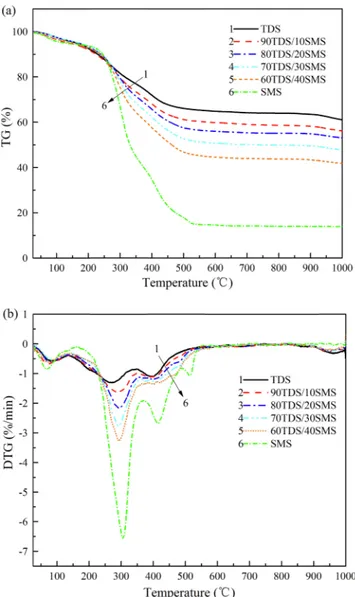
This study focused on the (co-)combustion properties of TDS and SMS at the heating rates of 10, 20 and 30 °C/min. Their (D)TG curves at 10 °C/min of the blends are located in between those of the individual solid fuels (Fig. 1). The significantly increased responses of mass loss and mass loss rate to the increased SMS fraction showed its more flammable substance and better combustion performance than TDS. Three and four peaks were observed in the DTG curves of TDS and SMS, respectively, due to the thermal degradations of their various compo-nents in the range of room temperature to 1000 °C (Fig. 1).
The first peak at about 80 °C and the mass loss below 200 °C mainly resulted from the evaporation of moisture which was not further dis-cussed in this study. At about 200 °C, the higher mass loss rate of TDS than SMS indicated the better decomposition behaviors of TDS at the low temperature, as was verified by the lower ignition temperature (Ti)
of TDS (197.2 °C) than SMS (256.8 °C) (Table 2). Similarly, TDS was reported to contain the small-molecule organic compounds with weak
chemical bonds that were easily biodegradable at a lower temperature (Peng et al., 2015). This finding supported the result that the volatiles matters of TDS were easily degraded at the lower temperature. SMS, a lignocellulosic material rich in (hemi)celluloses and lignin with a stable chemical structure, only began to degrade in the range of 220–550 °C. The maximum mass loss rates (−RP) of TDS and SMS were
esti-mated at 1.31 and 6.68%/min at 270.4 and 307.0 °C, respectively. The decompositions of the small-molecule organic compounds of TDS, and (hemi)celluloses of SMS marked the main stages of mass losses. The mass loss of TDS between 350 and 600 °C may have resulted from the combustion of the macromolecule organic matter produced during the stabilization and biological treatment stages (Peng et al., 2015). The combustion of SMS was finished at 600 °C, while a small mass loss of TDS occurred between 900 and 1000 °C due to the decomposition of inorganic substances. The TDS ash mainly contained alkali (Na2O),
al-kaline earth metals (e.g., CaO and MgO), Fe2O3, SiO2, and richer heavy
metals (e.g., Zn, Pb, Cu, Ni, and Cr). Pb, and Zn were reported to vo-latize at 940 °C, while CaSO4 tended to degrade in the range of
800–1000 °C, but alkali and alkaline earth metals reacted with the trace elements at a higher temperature (Guo and Zhong, 2018a; Wang et al., 2008). This may account for the changes in the (D)TG curves of TDS and its blends at the high temperatures.
3.3. Comparative indices of co-combustion performances
A strong linear relationship was found between the blend ratio and the maximum mass loss rate (−RP). The addition of SMS to TDS
in-creased the −RP, thermal reactivity and −RVvalues. The combustion
of volatiles in turn generated more heat to accelerate the decomposition of incombustible materials. The contrasting effects on Tiand Tbwere
observed with the increased SMS (Table 2). The addition of SMS in-creased Tiand decreased Tb. The lack of a linear growth trend in Tiand
Tbwith the increased SMS may suggest a synergistic effect on the
co-combustion. Their co-combustion improved the Tiand Tbproperties of
each other. The addition of more SMS changed the volatiles content, and thus, caused a less residual amount. Whether or not an interaction existed between SMS and TDS still remains to be explored in the next sections.
The significantly increased Di, Dband CCI with the increased SMS
indicated its improvement of the TDS combustion. This result was supported by the other findings (Guo and Zhong, 2018b; Peng et al., 2015). According to Eq.(1), the main control over Diby −RPin turn
depended on the amount of volatiles matters. More heat releases with the higher SMS content improved the combustion properties of TDS. The lower CCI values of TDS (1.11 × 10⁻⁸%2min−2°C−3) than SMS
(11.45 × 10⁻⁸%2min−2°C−3) at 10 °C/min pointed to the better
combustion performance of SMS than TDS. The CCI value of SMS was higher than that of camellia seed shell (8.15 × 10⁻⁸%2min−2°C) and
rapeseed meal (2.75 × 10⁻⁸%2min−2°C) (Chen et al., 2017b). An
ex-ponential relationship was found between CCI and blend ratio. 3.4. Interaction effects of blends
The interaction effect of the co-combustion means the involvement of the non-linear reaction mechanisms and not the simple sum of the additive effects of the individual biofuels. In the evaluation of the in-teractions, the experimental and theoretical TG and DTG curves were compared inFig. 2. The theoretical curves were based on the following equation (Peng et al., 2015):
= +
(D)TGcal SMS·(D)TGSMS TDS·(D)TGTDS (13) where γSMS and γTDSrepresent SMS and TDS fractions of the blends,
while (D)TGSMSand (D)TGTDSare the experimental curves of SMS and
TDS, respectively.
At below 350 °C, the similar rates of the experimental and theore-tical mass loss pointed to no significant interaction during the stages of
Fig. 1. (D)TG curves of TDS, SMS, and their blends at 10 °C /min. Table 2
Estimates of combustion characteristic parameters and indices from TG data at 10oC/min as a function of SMS fraction of blends.
SMS fraction of blends 0% 10% 20% 30% 40% 100% Ti(°C) 197.2 203.0 218.8 232.6 238.2 256.8 Tb(°C) 970.0 955.4 948.8 944.0 928.2 522.4 Tp(°C) 270.4 290.0 293.2 291.4 292.8 307.0 ΔT1/2(°C) 259.8 230.6 189.2 94.8 89.6 70.0 Δt1/2(min) 25.44 22.70 18.73 9.41 8.90 6.89 −Rv(%/min) 0.41 0.46 0.50 0.54 0.60 0.90 −RP(%/min) 1.31 1.64 2.16 2.77 3.26 6.68 CCI (10−8%2min−2°C−3) 1.11 1.49 1.90 2.27 2.87 11.45 Di(10−3%/min3) 3.15 3.56 4.25 4.78 5.46 9.79 Db(10−4%/min4) 0.23 0.30 0.47 1.17 1.48 6.71 Mf(%) 62.21 56.18 53.10 47.81 41.86 13.85
ΔT1/2: temperature range between the half -RP; -Rv: mean mass loss rate; and Mf:
water evaporation and volatiles combustion. In the range of 350–600 °C, the theoretical DTG curve of SMS exhibited a distinct weight loss peak, as with the experimental one. This suggested that some substances in TDS may hinder the combustion of fixed carbon in SMS and may promote the decomposition at a higher temperature. This case was supported by the interaction reported between 400 and 600 °C by Wang et al. (2011) that the partly absorbed heat from the SMS combustion adversely affected its combustion.
The mineral contents (e.g., Ca, K, and Mg) were found to produce a catalytic effect on the co-combustion of coke (Liu et al., 2013). The ash compositions of TDS and SMS (Table 1) showed that the minerals most probably acted as the catalyst. The catalytic effects can be weakened by the formation of the inactive alkali aluminosilicates, and the inactivated reactions between alkali metals and aluminosilicate minerals (Xie et al., 2018a). Hence, the interaction between TDS and SMS was more pro-nounced and complex in the co-combustion stage of fixed carbon.
The temperature of the maximum peak of mass loss (TP) of the
ex-perimental curves was slightly lower than that of the theoretical curves due to the interaction between the fuels. The heat release from the combustion of volatiles matters appeared to accelerate the TDS de-composition and lowered the peak temperature. At 480 °C, the experi-mental DTG curve had a small shoulder peak, while the theoretical DTG curve exhibited a small peak at 520 °C. The decomposition peak moved to a lower temperature zone. This case may be attributed to the inter-action between alkaline earth metals and metals of TDS and SMS so as to form a low melting point substance, thereby promoting the decom-position of the blends (Hu et al., 2015).
At 600 °C, the experimental and theoretical DTG curves were basi-cally consistent, and the combustion was almost completed. The still unclear interaction mechanism of TDS and SMS may be explained in the following two possible ways (Deng et al., 2016; Guo and Zhong, 2018b). First, the heat release from the volatiles of SMS in the low temperature may promote the TDS decomposition. Second, biochar formed during the SMS decomposition can catalyze the TDS decom-position. Silicates, aluminates, and metal salts may also catalyze the decomposition of the two substances. However, the lower residues of the theoretical than experimental TG curves with some blends indicated that some blends may cause an incomplete combustion. This inhibition effect may be due to the fact that SMS was easily decomposed at the lower temperatures accumulating large amounts of residues on the surface of TDS where the accumulation and condensation reactions acted to hinder or delay its decomposition (Chen et al., 2017a). To further discuss the co-combustion performance, the kinetic and ther-modynamic analyses conducted are presented in the next sections. 3.5. Kinetic and thermodynamic characterizations of co-combustion performances
Apparent activation energy can be defined as the energy barriers for a chemical reaction to overcome. A single mechanism function is not suitable to describe the complex co-combustion processes. In order to obtain an accurate Ea, the two iso-conversional methods (FWO and
KAS) were applied to the TG data at 10, 20 and 30 °C/min. Moisture became influential on the estimation of Ea at α = 0.1, while mass Fig. 2. A comparison of experimental versus theoretical TG-DTG curves with different SMS fractions.
transfer grew dominant in its estimation at α = 0.9. Therefore, the Ea
values were estimated in the range of 0.2–0.8. The Eaestimates by the
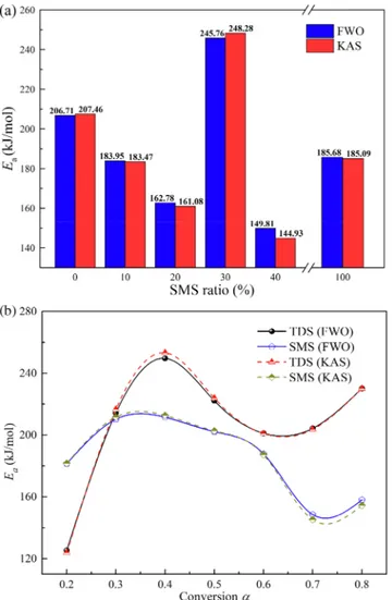
two methods were very close regardless of the blend ratio, with the high R2values of over 0.93 (Fig. 3). The similar trends in E
awere exhibited
with the increased α according to both FWO and KAS during the mono-combustions (Fig. 3b). α-dependent Eavalues pointed to the
involve-ment of the complicated reaction mechanisms in the co-combustion process (Barbanera et al., 2018).
The initially low Eavalues of both TDS and SMS indicated their less
energy requirement to start the chemical reaction (Fig. 3b). However, the lower Eavalue of TDS than SMS at α = 0.2 was due to the thermal
stability. Such contents of TDS as dyes, slurries, dyeing auxiliaries, acids, bases, fibers, inorganic compounds, and labile chemical struc-tures to be decomposed at high temperastruc-tures lowered its energy re-quirement (Peng et al., 2015). The increased Eavalues between 0.2 and
0.4 may be due to the decompositions of carbohydrates and proteins in TDS and SMS, thus decreasing the CeO and CeH bonds. Since these chemical bonds have poor thermal stability, their reduction was re-ported to elevate the Ea values (Cao et al., 2016). In the ranges of
0.4–0.6 (277.0–352.4 °C) for TDS and 0.4–0.7 (302.8–377.4 °C) for SMS, the Eavalues significantly declined. At these stages, the
decom-position and release of volatiles may have formed a porous carbon structure which enhanced the diffusion of oxygen (Wang et al., 2016). In the final reaction stage, the reason for the slight increase in Ea
may be due to the decompositions of biochar, and the high boiling point inorganic compounds which required high energy (Cao et al., 2016; Hu
et al., 2015). The lower average Eaestimate by FWO of SMS than TDS
(Fig. 3a) appeared to stem from the thermal stability. The increased SMS did not necessarily decrease the average Eavalue all the time. The
mean Eapeaked (245.76 kJ/mol) with 30% SMS but was minimized
(149.81 kJ/mol) with 40% SMS. In other words, the ease of the reaction with 40% SMS requiring less energy to promote the co-combustion process appeared to be the optimal choice of the blend ratio.
Table 3shows the multiple comparisons of Ea, A, ΔH, ΔG, and ΔS as
a function of the blend ratio and the conversion degree during the (co-) combustion process. The variation in the A values of the blends with the conversion rate by more than 109s−1pointed to the complex
compo-sitions and combustion reactions (Maia and Morais, 2016). The A range was wider by several orders of magnitude for TDS than SMS. 40% SMS led to the narrowest range of A. The small difference between the Ea
and ΔH values by < 7 kJ/mol (Table 3) showed that the reactions benefited the formation of the activated complex (Barbanera et al., 2018; Müsellim et al., 2018). The lower the ΔG value is, the more fa-vorable the reaction is (Hui et al., 2015). The average ΔG value was lower for TDS (136.69 kJ/mol) than SMS (147.30 kJ/mol). Their mean values were lower than those of rice straw (164.59 kJ/mol) and rice bran (167.17 kJ/mol) which showed the less heat requirements of their combustion reactions (Maia and Morais, 2016). The negative ΔS and positive ΔG values also demonstrated that the combustions of these substances involved a non-spontaneous reaction.
3.6. Reaction mechanisms of degradation of volatiles
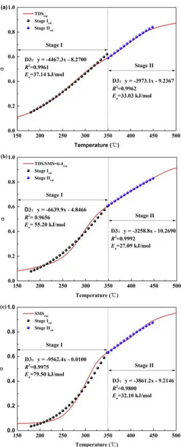
The reaction mechanisms of the individual biofuels, and 60TDS/ 40SMS were determined using the CR method for the releases of vo-latiles, and the char-burning stage. Based on the 17 common reaction models, the diffusion model, also known as the three-dimensional dif-fusion model (D3), was determined as the most suitable reaction me-chanism with the highest R2. All the R2values were above 96% when
the D3 model was used though from the different heating rates and samples (Table 4). The good match between the calculated and ex-perimental α (Fig. 4) indicated the reliability of the D3 model. The D3 model was shown to well describe the decomposition of lignocellulosic materials at the low temperature (Mallick et al., 2018). Fernandez-Lopez et al. (Fernandez-Lopez et al., 2016) found that the D3 model matched well with the devolatilization stage of manure and performed well in the reconstruction of the DTG curves. The D3 model was ap-propriate in the stages of devolatilization (180–350 °C) and char com-bustion (350–450 °C) for all the samples and heating rates (Table 4). The Eaestimates by the CR method were lower than those of the
iso-conversional methods, as discussed in Section 3.5. The Eaestimates
from the model-free methods can be more reliable and should change as a function of α due to the complicated reactions of the entire combus-tion process. The Eaestimates by the CR method were the average
va-lues of the specific decomposition stages. 3.7. Response surface methodology 3.7.1. Modeling
The significance and adequacy of the best-fit quadratic models of ML and MLR according to BBD (Table 5) were evaluated using analysis of variance (ANOVA) (Joshi et al., 2018). The ANOVA results for the quadratic model of ML are shown inTable 6.
The best-fit quadratic regression model is provided below in terms of the coded factors:
= + +
+ + + +
ML(%) 53.64 0.85A 7.26B 20.39C 0.27AB 0.004AC 4.95BC 1.35A2 0.60B2 18.98C2
The model predictors with a p-value < 0.05 were blend ratio, temperature, and quadratic temperature (Table 6). The lack-of-fit p value > 0.05 indicated that the model accurately fitted the ML data
Fig. 3. Relationships between (a) apparent activation energy (Ea) and SMS
fraction; and (b) Eaand conversion degree (α) based on the FWO and KAS
(Lin et al., 2018). The model accounted for 91.9% of variation in ML. Based on the one-leave-out cross-validation, the predictive power (R2
pred) of the model was also high (80.42%). Precision measures the
signal-to-noise (S/N) ratio whose value being > 4 is considered
desirable in which case this value for our model was 13.5. The coeffi-cient of variation value of 8.39% demonstrated the good degree of precision and accuracy of the model (Joshi et al., 2018).
Our multiple non-linear regression results pointed to the quadratic
Table 3
Multiple comparisons of one kinetic and four thermodynamic parameters as a function of blend ratio of TDS to SMS, and conversion degree (α) according to FWO and KAS methods..
Samples α FWO KAS
Ea(kJ/mol) R2 A (s−1) ΔH (kJ/
mol) ΔG (kJ/mol) ΔS (J/mol) Ea(kJ/mol) R
2 A (s−1) ΔH (kJ/
mol) ΔG (kJ/mol) ΔS (J/mol) TDS 0.2 125.39 0.9488 5.75E + 11 121.41 138.86 -32.11 123.78 0.9424 3.97E + 11 119.80 138.92 -35.18 0.3 214.27 0.9747 3.42E + 20 209.95 136.44 135.26 216.61 0.9727 5.81E + 20 212.30 136.39 139.66 0.4 249.62 0.9337 9.96E + 23 245.05 135.75 201.10 253.28 0.9292 2.27E + 24 248.70 135.68 207.95 0.5 222.20 0.8771 2.06E + 21 217.36 136.28 149.19 223.90 0.8675 3.01E + 21 219.05 136.24 152.36 0.6 201.12 0.9171 1.75E + 19 195.91 136.73 108.90 200.96 0.9090 1.69E + 19 195.75 136.73 108.59 0.7 204.29 0.9527 3.59E + 19 198.76 136.66 114.26 203.62 0.9477 3.08E + 19 198.09 136.67 113.00 0.8 230.11 0.9488 1.22E + 22 224.24 136.12 162.15 230.11 0.9437 1.22E + 22 224.25 136.12 162.15 90TDS/10SMS 0.2 120.93 0.9444 7.58E + 10 116.88 144.54 -49.11 118.95 0.9370 4.88E + 10 114.90 144.61 -52.77 0.3 187.09 0.9629 1.61E + 17 182.69 142.49 71.39 187.86 0.9595 1.91E + 17 183.47 142.47 72.80 0.4 209.41 0.9450 2.12E + 19 204.77 141.96 111.53 210.83 0.9403 2.89E + 19 206.20 141.93 114.13 0.5 208.35 0.9511 1.68E + 19 203.49 141.99 109.22 209.26 0.9467 2.05E + 19 204.40 141.97 110.87 0.6 181.40 0.9072 4.63E + 16 176.23 142.64 59.66 180.29 0.8973 3.63E + 16 175.12 142.67 57.64 0.7 181.37 0.9325 4.59E + 16 175.85 142.64 58.98 179.54 0.9245 3.08E + 16 174.03 142.69 55.66 0.8 199.14 0.9685 2.25E + 18 193.28 142.20 90.71 197.54 0.9647 1.58E + 18 191.68 142.24 87.81 80TDS/20SMS 0.2 150.27 0.9986 4.10E + 13 146.06 144.41 2.90 149.48 0.9984 3.44E + 13 145.26 144.44 1.45 0.3 180.16 0.9978 2.81E + 16 175.66 143.56 56.68 180.33 0.9976 2.91E + 16 175.83 143.56 56.98 0.4 181.60 0.9929 3.84E + 16 176.90 143.52 58.95 181.45 0.9922 3.72E + 16 176.75 143.53 58.67 0.5 178.69 0.9876 2.04E + 16 173.80 143.60 53.34 178.00 0.9863 1.75E + 16 173.11 143.62 52.08 0.6 155.93 0.9399 1.41E + 14 150.77 144.24 11.54 153.50 0.9321 8.31E + 13 148.34 144.31 7.12 0.7 150.12 0.9542 3.96E + 13 144.62 144.42 0.36 146.68 0.9475 1.87E + 13 141.19 144.53 -5.90 0.8 142.65 0.9682 7.70E + 12 136.82 144.66 -13.85 138.12 0.9629 2.85E + 12 132.29 144.81 -22.11 70TDS/30SMS 0.2 425.84 0.9997 4.09E + 39 421.50 139.02 500.41 439.10 0.9997 7.10E + 40 434.76 138.88 524.14 0.3 278.26 1.0000 5.89E + 25 273.69 141.02 235.02 283.39 1.0000 1.79E + 26 278.82 140.93 244.27 0.4 236.28 0.9960 6.52E + 21 231.54 141.79 159.00 238.90 0.9957 1.15E + 22 234.17 141.73 163.75 0.5 234.18 0.9946 4.14E + 21 229.27 141.83 154.91 236.34 0.9942 6.62E + 21 231.43 141.78 158.81 0.6 207.59 0.9583 1.27E + 19 202.41 142.39 106.32 207.83 0.9542 1.34E + 19 202.66 142.39 106.77 0.7 180.98 0.9698 3.81E + 16 175.46 143.04 57.43 179.11 0.9661 2.53E + 16 173.59 143.09 54.03 0.8 157.17 0.9783 2.07E + 14 151.29 143.70 13.45 153.32 0.9749 8.91E + 13 147.44 143.82 6.43 60TDS/40SMS 0.2 139.55 0.9997 3.99E + 12 135.18 144.65 -16.73 137.88 0.9996 2.76E + 12 144.71 133.51 -19.78 0.3 153.93 0.9993 9.35E + 13 149.35 144.19 9.12 152.57 0.9992 6.94E + 13 144.23 147.99 6.64 0.4 155.84 0.9994 1.42E + 14 151.11 144.13 12.33 154.27 0.9994 1.01E + 14 144.18 149.53 9.46 0.5 165.22 0.9997 1.11E + 15 160.32 143.86 29.09 163.79 0.9997 8.10E + 14 143.90 158.89 26.50 0.6 157.55 0.9966 2.06E + 14 152.40 144.08 14.70 138.30 0.9941 3.03E + 12 144.69 133.16 -20.39 0.7 142.18 0.9949 7.10E + 12 136.68 144.56 -13.93 138.30 0.9941 3.03E + 12 144.69 132.80 -21.01 0.8 134.43 0.9929 1.29E + 12 128.57 144.83 -28.73 129.38 0.9917 4.26E + 11 145.01 123.52 -37.97 SMS 0.2 181.48 0.9978 1.42E + 16 176.96 147.37 51.00 181.69 0.9976 1.49E + 16 177.16 147.37 51.37 0.3 210.19 0.9990 6.35E + 18 205.52 146.66 101.46 211.58 0.9989 8.53E + 18 206.91 146.63 103.92 0.4 211.50 0.9598 8.39E + 18 206.71 146.63 103.57 212.73 0.9562 1.09E + 19 207.94 146.61 105.74 0.5 202.22 0.8196 1.17E + 18 197.31 146.85 86.99 202.73 0.8050 1.30E + 18 197.83 146.84 87.90 0.6 187.80 0.9326 5.46E + 16 182.72 147.21 61.22 187.19 0.9254 4.80E + 16 182.11 147.22 60.15 0.7 148.57 0.9844 1.27E + 13 143.16 148.34 −8.92 145.20 0.9818 6.17E + 12 139.80 148.45 −14.91 0.8 158.00 0.9640 9.54E + 13 152.29 148.04 7.32 154.50 0.9585 4.51E + 13 148.78 148.15 1.09 Table 4
(Co-)combustion kinetic models of two stages at three heating rates.
Sample β (°C/min) Devolatilization stage (D3) Char combustion stage (D3)
Equation R2 E
a(kJ/mol) Equation R2 Ea(kJ/mol)
TDS 10 y = −4467.3x – 8.2700 0.9961 37.14 y = −3973.1x – 9.2367 0.9962 33.03 20 y = −8806.5x – 0.2706 0.9908 68.67 y = −3652.2x – 9.8898 0.9893 30.36 30 y = −8833.4x – 0.2609 0.9915 69.55 y = −3456.1x – 10.2080 0.9885 28.73 60TDS/40SMS 10 y = −6639.9x – 4.8466 0.9656 55.20 y = −3258.8x – 10.2690 0.9992 27.09 20 y = −9283.6x – 0.1710 0.9959 77.18 y = −2993.1x – 10.8570 0.9992 24.88 30 y = −9403.6x – 0.1627 0.9963 78.18 y = −2921.8x – 11.0410 0.9989 24.29 SMS 10 y = −9562.4x – 0.0100 0.9975 79.50 y = −3861.2x – 9.2146 0.9800 32.10 20 y = −9811.5x + 0.0299 0.9964 81.57 y = −3363.3x – 10.1110 0.9747 27.96 30 y = −9836.7x – 0.1143 0.9271 81.78 y = −10224x – 0.0035 0.9990 85.00
model as the best-fit one with the following coded factors:
= + +
+ + +
MLR (%/min) 0.22 0.32A 0.094B 0.44C 0.49AB 0.11AC 0.054BC 0.006A2 0.030B2 0.72C2
where A, B and C refer to heating rate (°C/min), blend ratio (%), and temperature (°C), respectively. The model elucidated 76.95% of varia-tion in MLR, with an R2
predof 54.6%. The optimal operational values
were estimated at 15.90 °C/min for heating rate, 60/40% for the TDS/ SMS ratio, and 867.0 °C for ML and 30 °C/min, 60/40% and 1000 °C for MLR. These conditions were consistent with the conclusions drawn in Sections 3.5. Under the optimal conditions, the maximized ML and MLR values were determined as 38.29% and 47.43%/min, respectively. 3.7.2. Effects of operational parameters
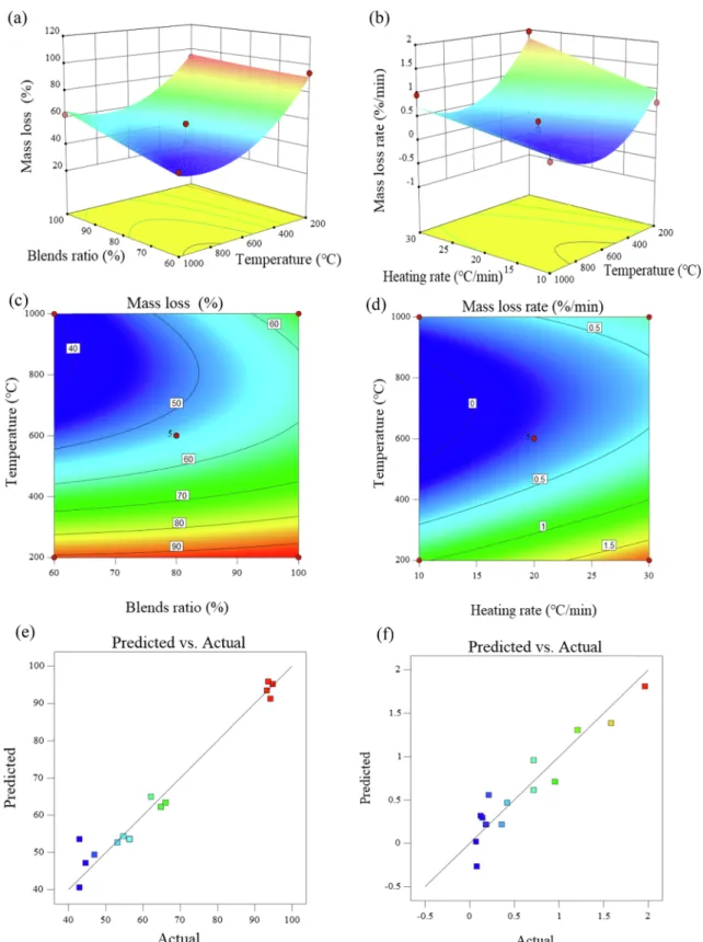
The significant predictors of ML and MLR determined in this study were consistent with the results by (Liu et al., 2017). Their effects on the response variables are depicted inFig. 5. According to the effects of the blend ratio and temperature on ML (Fig. 5a), the ML value was maximized with the increased temperature, and the low TDS fraction at
Fig. 4. Calculated versus experimental α using the D3 model at 10 °C/min.
Table 5
Box-Behnken design of three variables, and a comparison of experimental (exp) versus predicted (pred) responses of ML and MLR.
Variables Symbol Ranges and levels
Low Mid High Heating rate (°C/min) A 10 20 30 Blend ratio (%) B 60 80 100 Temperature (°C) C 200 600 1000 Std Run A B C ML (%) MLR (°C/min)
Exp Pred Exp Pred 1 1 10 60 600 44.55 47.22 0.080 −0.264 17 2 20 80 600 56.32 53.64 0.184 0.219 7 3 10 80 1000 53.12 52.74 0.144 0.295 9 4 20 60 200 94.20 91.30 1.208 1.309 5 5 10 80 200 93.27 93.51 0.716 0.958 12 6 20 100 1000 62.13 65.03 0.716 0.615 13 7 20 80 600 56.32 53.64 0.184 0.219 10 8 20 100 200 93.64 95.92 1.582 1.388 11 9 20 60 1000 42.90 40.62 0.125 0.319 16 10 20 80 600 42.90 53.64 0.358 0.219 15 11 20 80 600 56.32 53.64 0.184 0.219 14 12 20 80 600 56.32 53.64 0.184 0.219 8 13 30 80 1000 54.66 54.42 0.954 0.711 4 14 30 100 600 66.09 63.42 0.213 0.556 2 15 30 60 600 46.93 49.44 0.419 0.468 3 16 10 100 600 64.78 62.26 0.070 0.021 6 17 30 80 200 94.83 95.23 1.962 1.812
Std: Standard run order; and Run: Random run order. Table 6
Analysis of variance (ANOVA) results for mass loss (ML, %).
Source SS df MS F-value p-value VIF Intercept 5405.14 9 600.57 21.18 0.0003 A (heating rate) 5.74 1 5.74 0.20 0.6662 1 B (blend ratio) 421.28 1 421.28 14.86 0.0062 1 C (temperature) 3326.55 1 3326.55 117.34 < 0.0001 1 A * B 0.28 1 0.28 0.01 0.9230 1 A * C 0.00 1 0.00 0.00 0.9986 1 B * C 97.97 1 97.97 3.45 0.1054 1 A2 7.73 1 7.73 0.27 0.6177 1 B2 1.50 1 1.50 0.05 0.8246 1 C2 1517.28 1 1517.28 53.50 0.0002 1 Residual 198.50 7 28.36 Lack of fit 54.50 3 18.17 0.50 0.6996 Pure error 144.00 4 36.00 Total 5603.64 16 SD 5.32 R2 adj(%) 91.90 Mean 63.49 R2 pred(%) 80.42 CV (%) 8.39 Precision 13.5 PRESS 1096.98
df: degrees of freedom; SS: sum of squares; MS: mean squares; VIF: variation inflation factor; F-value: Fisher test value; p-value: significance level; SD: standard deviation; CV: coefficient of variation; PRESS: predicted residual sum of squares.
20 °C/min. No significant difference was found at the low temperature despite the addition of more SMS. This suggested that the interaction between the blend ratio and temperature existed at the high tempera-tures.
Fig. 5b shows the increased MLR with the increased heating rate due to its more energy supply as well as the higher MLR at the low tem-peratures due to the combustion of volatiles matters. Fig. 5c and d suggest that the SMS fraction and temperature should be over 42% and 750 °C, respectively. MLR was close to zero in the range of 500–850 °C
at below 15 °C/min (Fig. 5d). This was consistent with the DTG curve in Section 3.1. Fig. 5e and f show that the quadratic model was more suitable to describe ML than MLR as was also verified by their R2values
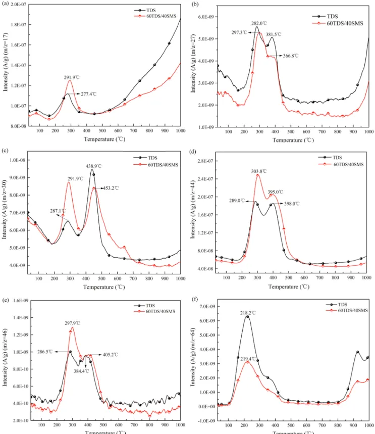
of 96.46 and 89.92%, respectively. 3.8. TG-MS analysis
The emissions of pollutant gases from TDS and 40% SMS were analyzed using TG-MS data.Fig. 6shows the intensity changes in NH3 Fig. 5. (a and b) 3D surface, (c and d) contour and (e and f) predicted versus actual value plots for effects of significant variables on ML and MLR.
(m/z = 17), HCN (m/z = 27), NO (m/z = 30), CO2 (m/z = 44), NO2
(m/z = 46), and SO2(m/z = 64). Their emission peaks were all located
in the range of 200–500 °C. HCN and NH3are the intermediate species
to form NOxduring the combustion of the fuel N, and their emissions
were significant to evaluate the transformation of N species (Shah et al., 2018).Fig. 6a and b showed that with the addition of 40% SMS to TDS, the emission peak of NH3and HCN moved toward a higher temperature
which indicated the higher binding energy and stronger stability of
N-containing compounds in SMS (Gong et al., 2019).Li and Tan (2000) stated that HCN was mainly generated from the decomposition of N-containing structures with low thermal stability, while thermally stable N-containing structures controlled the generation of NH3. However, our
results showed the higher emission intensity and easier emission peak of NH3than HCN during the devolatilization stage. This finding was
consistent with other results that more NH3was released directly prior
to HCN during the devolatilizing stage of biomass combustion, thus
leading to the partial transformation of NH3into HCN according to the
following reaction: NH3+ CH → HCN (Fig. 6a and b) (Moroń and Rybak, 2015; Shah et al., 2018). The addition of 40% SMS accelerated the NH3emission and lowered the HCN emission. The higher H content
of SMS than TDS seemed to provide more H radicals to promote the NH3emission from the devolatization stage (Li and Tan, 2000). The N
contents of fuel and remaining char were reported to result in more NH3
and HCN releases at above 800 °C (Aho et al., 1993; Zhou et al., 2018). There were the two peaks of NO and NO2emissions for TDS, while
the first peak temperature was slightly lower for NO (284.6 °C) than NO2(288.4 °C) (Fig. 6c and e). This trends also existed with 40% SMS.
NO is known to be the predominant N-containing gaseous species when the oxidation of NO to NO2in the air atmosphere occurs easily in a high
atmospheric pressure and at a low temperature (Wang et al., 2018a). The NO formation involved a complex process mainly depending on the fuel type and the combustion conditions, while the main source of NO was the oxidation of fuel-bound N at below 1500 °C in a combustion system (Yanik et al., 2018). The strengthened first emission peaks of NO and NO2, and their weakened second peaks with 40% SMS indicated
more NOx releases from the stages of volatiles combustion and
in-organic N decomposition at below 300 °C (Tian et al., 2013). The maximum emission peak of SMS at 540 °C reported by our previous study (Huang et al., 2018) did not appear in the present study sug-gesting an interaction to accelerate the char combustion, and the re-lease of more NOxemissions.Fig. 6d shows the CO2emission with the
risen temperature whose two peaks representing the combustions of volatiles matters and fixed carbon, respectively. 40% SMS enhanced the CO2emission, in particular, for the first peak due to its higher C content
than TDS (Table 1).
Fig. 6f shows that 40% SMS decreased the intensity of SO2emission
due to its low S content. The first peak of SO2at 220 °C for TDS and 40%
SMS indicated that most S existed in the form of organic S that was released upon the combustion of volatiles matters. The emission peak of SO2 at 320 °C according to our previous study (Huang et al., 2018)
suggested that the S content of TDS had lower thermal stability, as was consistent with the lower ignition activation energy of TDS than SMS. The increased SO2emission at above 800 °C showed that the
in-organic S decomposed at the high temperature. The intensity of TDS with 40% SMS was lower than that of the pure TDS due to the lower inorganic S. The additional peak of SO2at about 900 °C appeared to
relate to the decomposition of CaSO4or other inorganic S-containing
structures such as Na2SO4. Since TDS contained a large amount of Na
and Si, the following reaction at the high temperature may occur to promote the generation of SO2: Na2SO4+ 6SiO2+ Al2O3→
2NaAlSi3O8+ SO2+ 0.5O2(Qi et al., 2018). CaO as a common
disin-fectant found in SMS can effectively absorb SO2to form CaSO4. CaSO4
decomposes to CaO and SO2between 800 and 1000 °C according to the
following equation: CaSO4→ CaO + SO2 (Wang et al., 2008; Yanik et al., 2018). According toTable 1, the high P content of SMS may promote the degradation of CaSO4 following the reaction:
3CaSO4+ P2O5→ Ca3(PO4)2+ 3SO2+ 1.5O2(Qi et al., 2018). Hence,
with Ca and P present in the combustion system at the high tempera-ture, it is easier to generate more SO2. At low-to-moderate
tempera-tures, the organic S was thermally decomposed during the devolatili-zation stage, while the inorganic S was shown to decompose through interaction with the matrix at above 900 °C (Ren et al., 2017). The SO2
emission peak at the high temperature was consistent with the (D)TG curves that a small amount of inorganic matters was degraded at above 900 °C.
4. Conclusions
The addition of SMS to TDS significantly increased –RP, Di, Db, and
CCI, indicative of the improved co-combustion performance. The thermal degradation lowered Tiby 59.6 °C for TDS relative to SMS. The
interaction occurred mainly between 350 and 600 °C during the
combustion stage of fixed carbon, and that the minerals may have catalyzed the combustion process. The minimum mean Ea obtained
with 40% SMS pointed to it as the optimal blend ratio. The addition of 40% SMS to TDS decreased the HCN and SO2emissions but released
more NO and NO2emissions at the lower temperature.
Acknowledgments
This research was financially supported by the National Natural Science Foundation of China (No. 51608129), the Scientific and Technological Planning Project of Guangzhou, China (Nos. 201704030109 and 2016201604030058), and the Science and Technology Planning Project of Guangdong Province, China (Nos. 2019B020208017, 2018A050506046, 2015B020235013, 2017A050501036 and 2016A050502059).
Appendix A. Supplementary material
Supplementary data to this article can be found online athttps:// doi.org/10.1016/j.biortech.2019.02.011.
References
Aho, M.J., Hämäläinen, J.P., Tummavuori, J.L., 1993. Importance of solid fuel properties to nitrogen oxide formation through HCN and NH3in small particle combustion.
Combust. Flame 95, 22–30.
Barbanera, M., Cotana, F., Di Matteo, U., 2018. Co-combustion performance and kinetic study of solid digestate with gasification biochar. Renew. Energy 121, 597–605.
Buyukada, M., 2017b. Uncertainty estimation by Bayesian approach in thermochemical conversion of walnut hull and lignite coal blends. Bioresour. Technol. 232, 87–92.
Buyukada, M., 2017a. Probabilistic uncertainty analysis based on Monte Carlo simula-tions of co-combustion of hazelnut hull and coal blends: Data-driven modeling and response surface optimization. Bioresour. Technol. 225, 106–112.
Cai, J., Xu, D., Dong, Z., Yu, X., Yang, Y., Banks, S.W., Bridgwater, A.V., 2018. Processing thermogravimetric analysis data for isoconversional kinetic analysis of lignocellulosic biomass pyrolysis: case study of corn stalk. Renew. Sust. Energy Rev. 82, 2705–2715.
Cao, L., Yuan, X., Jiang, L., Li, C., Xiao, Z., Huang, Z., Chen, X., Zeng, G., Li, H., 2016. Thermogravimetric characteristics and kinetics analysis of oil cake and torrefied biomass blends. Fuel 175, 129–136.
Chen, C., Qin, S., Chen, F., Lu, Z., Cheng, Z., 2017a. Co-combustion characteristics study of bagasse, coal and their blends by thermogravimetric analysis. J. Energy Inst.
https://doi.org/10.1016/j.joei.2017.12.008.
Chen, J., Wang, Y., Lang, X., Ren, X., Fan, S., 2017b. Comparative evaluation of thermal oxidative decomposition for oil-plant residues via thermogravimetric analysis: thermal conversion characteristics, kinetics, and thermodynamics. Bioresour. Technol. 243, 37–46.
Deng, S., Wang, X., Tan, H., Mikulčić, H., Yang, F., Li, Z., Duić, N., 2016.
Thermogravimetric study on the Co-combustion characteristics of oily sludge with plant biomass. Thermochim. Acta 633, 69–76.
Dong, H., Jiang, X., Lv, G., Wang, F., Huang, Q., Chi, Y., Yan, J., Yuan, W., Chen, X., Lu, W., 2017. Co-combustion of tannery sludge in a bench-scale fluidized-bed combustor: gaseous emissions and Cr distribution and speciation. Energy Fuels 31, 11069–11077.
Fernandez-Lopez, M., Pedrosa-Castro, G.J., Valverde, J.L., Sanchez-Silva, L., 2016. Kinetic analysis of manure pyrolysis and combustion processes. Waste Manage. 58, 230–240.
Gil, M.V., Casal, D., Pevida, C., Pis, J.J., Rubiera, F., 2010. Thermal behaviour and ki-netics of coal/biomass blends during co-combustion. Bioresour. Technol. 101, 5601–5608.
Gong, Z., Wang, Z., Wang, Z., Fang, P., Meng, F., 2019. Study on the migration char-acteristics of nitrogen and sulfur during co-combustion of oil sludge char and mi-croalgae residue. Fuel 238, 1–9.
Guo, F., Zhong, Z., 2018b. Optimization of the co-combustion of coal and composite biomass pellets. J. Clean. Prod. 185, 399–407.
Guo, F., Zhong, Z., 2018a. Co-combustion of anthracite coal and wood pellets: thermo-dynamic analysis, combustion efficiency, pollutant emissions and ash slagging. Environ. Pollut. 239, 21–29.
Hu, S., Ma, X., Lin, Y., Yu, Z., Fang, S., 2015. Thermogravimetric analysis of the co-combustion of paper mill sludge and municipal solid waste. Energy Convers. Manage. 99, 112–118.
Huang, J., Liu, J., Chen, J., Xie, W., Kuo, J., Lu, X., Chang, K., Wen, S., Sun, G., Cai, H., Buyukada, M., Evrendilek, F., 2018. Combustion behaviors of spent mushroom sub-strate using TG-MS and TG-FTIR: thermal conversion, kinetic, thermodynamic and emission analyses. Bioresour. Technol. 266, 389–397.
Hui, L., Niu, S.L., Lu, C.M., Cheng, S.Q., 2015. Comparative evaluation of thermal de-gradation for biodiesels derived from various feedstocks through transesterification. Energy Convers. Manage. 98, 81–88.
Jiang, L., Zhang, D., Li, M., He, J.-J., Gao, Z.-H., Zhou, Y., Sun, J.-H., 2018. Pyrolytic behavior of waste extruded polystyrene and rigid polyurethane by multi kinetics methods and Py-GC/MS. Fuel 222, 11–20.
karanja oil for production of biodiesel using ultrasound assisted approach with op-timization using response surface methodology. Chem. Eng. Process. 124, 186–198.
Latchubugata, C.S., Kondapaneni, R.V., Patluri, K.K., Virendra, U., Vedantam, S., 2018. Kinetics and optimization studies using response surface methodology in biodiesel production using heterogeneous catalyst. Chem. Eng. Res. Des. 135, 129–139.
Li, X.G., Lv, Y., Ma, B.G., Jian, S.W., Tan, H.B., 2011. Thermogravimetric investigation on co-combustion characteristics of tobacco residue and high-ash anthracite coal. Bioresour. Technol. 102, 9783–9787.
Li, C.-Z., Tan, L.L., 2000. Formation of NOx and SOx precursors during the pyrolysis of coal and biomass. Part III. Further discussion on the formation of HCN and NH3
during pyrolysis. Fuel 79, 1899–1906.
Lin, J., Su, B., Sun, M., Chen, B., Chen, Z., 2018. Biosynthesized iron oxide nanoparticles used for optimized removal of cadmium with response surface methodology. Sci. Total. Environ. 627, 314–321.
Liu, J., Huang, L., Buyukada, M., Evrendilek, F., 2017. Response surface optimization, modeling and uncertainty analysis of mass loss response of co-combustion of sewage sludge and water hyacinth. Appl. Therm. Eng. 125, 328–335.
Liu, Z., Zhang, Y., Zhong, L., Orndroff, W., Zhao, H., Cao, Y., Zhang, K., Pan, W.-P., 2013. Synergistic effects of mineral matter on the combustion of coal blended with biomass. J. Therm. Anal. Calorim. 113, 489–496.
Liu, Z., Zhang, T., Zhang, J., Xiang, H., Yang, X., Hu, W., Liang, F., Mi, B., 2018b. Ash fusion characteristics of bamboo, wood and coal. Energy 161, 517–522.
Liu, J., Zhuo, Z., Xie, W., Kuo, J., Lu, X., Buyukada, M., Evrendilek, F., 2018a. Interaction effects of chlorine and phosphorus on thermochemical behaviors of heavy metals during incineration of sulfur-rich textile dyeing sludge. Chem. Eng. J. 351, 897–911.
Ma, Q., Han, L., Huang, G., 2017. Potential of water-washing of rape straw on thermal properties and interactions during co-combustion with bituminous coal. Bioresour. Technol. 234, 53–60.
Maia, A.A.D., Morais, L.C.D., 2016. Kinetic parameters of red pepper waste as biomass to solid biofuel. Bioresour. Technol. 204, 157–163.
Mallick, D., Poddar, M.K., Mahanta, P., Moholkar, V.S., 2018. Discernment of synergism in pyrolysis of biomass blends using thermogravimetric analysis. Bioresour. Technol. 261, 294–305.
Moroń, W., Rybak, W., 2015. NOx and SO2emissions of coals, biomass and their blends
under different oxy-fuel atmospheres. Atmos. Environ. 116, 65–71.
Müsellim, E., Tahir, M.H., Ahmad, M.S., Ceylan, S., 2018. Thermokinetic and TG/DSC-FTIR study of pea waste biomass pyrolysis. Appl. Therm. Eng. 137, 54–61.
Peng, X., Ma, X., Xu, Z., 2015. Thermogravimetric analysis of co-combustion between microalgae and textile dyeing sludge. Bioresour. Technol. 180, 288–295.
Qi, X., Song, G., Song, W., Yang, S., Lu, Q., 2018. Combustion performance and slagging
characteristics during co-combustion of Zhundong coal and sludge. J. Energy. Inst. 91, 397–410.
Ren, X., Sun, R., Meng, X., Vorobiev, N., Schiemann, M., Levendis, Y.A., 2017. Carbon, sulfur and nitrogen oxide emissions from combustion of pulverized raw and torrefied biomass. Fuel 188, 310–323.
Shah, I.A., Gou, X., Zhang, Q., Wu, J., Wang, E., Liu, Y., 2018. Experimental study on NOx emission characteristics of oxy-biomass combustion. J. Clean. Prod. 199, 400–410.
Shi, W., Kong, L.-X., Bai, J., Xu, J., Li, W., Bai, Z., Li, W., 2018. Effect of CaO/Fe2O3on
fusion behaviors of coal ash at high temperatures. Fuel Process. Technol. 181, 18–24.
Tian, Y., Zhang, J., Zuo, W., Chen, L., Cui, Y., Tan, T., 2013. Nitrogen conversion in relation to NH3and HCN during microwave pyrolysis of sewage sludge. Environ. Sci.
Technol. 47, 3498–3505.
Wang, Z., Hong, C., Xing, Y., Li, Y., Feng, L., Jia, M., 2018b. Combustion behaviors and kinetics of sewage sludge blended with pulverized coal: with and without catalysts. Waste Manage. 74, 288–296.
Wang, X., Jin, Y., Wang, Z., Mahar, R.B., Nie, Y., 2008. A research on sintering char-acteristics and mechanisms of dried sewage sludge. J. Hazard. Mater. 160, 489–494. Wang, C.A., Wang, P., Du, Y., Che, D., 2018a. Experimental study on effects of combus-tion atmosphere and coal char on NO2reduction under oxy-fuel condition. J. Energy
Inst.https://doi.org/10.1016/j.joei.2018.07.004.
Wang, G., Zhang, J., Shao, J., Liu, Z., Zhang, G., Xu, T., Guo, J., Wang, H., Xu, R., Lin, H., 2016. Thermal behavior and kinetic analysis of co-combustion of waste biomass/low rank coal blends. Energy Convers. Manage. 124, 414–426.
Wang, Q., Zhao, W., Liu, H., Jia, C., Li, S., 2011. Interactions and kinetic analysis of oil shale semi-coke with cornstalk during co-combustion. Appl. Energy 88, 2080–2087.
Xie, C., Liu, J., Zhang, X., Xie, W., Sun, J., Chang, K., Kuo, J., Xie, W., Liu, C., Sun, S., Buyukada, M., Evrendilek, F., 2018b. Co-combustion thermal conversion character-istics of textile dyeing sludge and pomelo peel using TGA and artificial neural net-works. Appl. Energy 212, 786–795.
Xie, C., Liu, J., Xie, W., Kuo, J., Lu, X., Zhang, X., He, Y., Sun, J., Chang, K., Xie, W., Liu, C., Sun, S., Buyukada, M., Evrendilek, F., 2018a. Quantifying thermal decomposition regimes of textile dyeing sludge, pomelo peel, and their blends. Renew. Energy 122, 55–64.
Yanik, J., Duman, G., Karlström, O., Brink, A., 2018. NO and SO2emissions from
com-bustion of raw and torrefied biomasses and their blends with lignite. J. Environ. Manage. 227, 155–161.
Zhou, H., Li, Y., Li, N., Qiu, R., Cen, K., 2018. Conversions of fuel-N to NO and N2O during
devolatilization and char combustion stages of a single coal particle under oxy-fuel fluidized bed conditions. J. Energy Inst.https://doi.org/10.1016/j.joei.2018.01.001.